A Multivariate Timeseries Modeling Approach to Severity of Illness Assessment and Forecasting in ICU with Sparse, Heterogeneous Clinical Data

Abstract

The ability to determine patient acuity (or severity of illness) has immediate practical use for clinicians. We evaluate the use of multivariate timeseries modeling with the multi-task Gaussian process (GP) models using noisy, incomplete, sparse, heterogeneous and unevenly-sampled clinical data, including both physiological signals and clinical notes. The learned multi-task GP (MTGP) hyperparameters are then used to assess and forecast patient acuity. Experiments were conducted with two real clinical data sets acquired from ICU patients: firstly, estimating cerebrovascular pressure reactivity, an important indicator of secondary damage for traumatic brain injury patients, by learning the interactions between intracranial pressure and mean arterial blood pressure signals, and secondly, mortality prediction using clinical progress notes. In both cases, MTGPs provided improved results: an MTGP model provided better results than single-task GP models for signal interpolation and forecasting (0.91 vs 0.69 RMSE), and the use of MTGP hyperparameters obtained improved results when used as additional classification features (0.812 vs 0.788 AUC).

1 Introduction

Motivation

Decisions in the intensive care unit (ICU) are frequently made in settings with a high degree of uncertainty based on a wide variety of data sources, such as vital signs, clinical notes, fluids, medications, etc. Clinical data collection is rapidly expanding, but these data are often sparse and irregularly sampled, and contaminated by a variety of noise interference and human error. The ICU is playing an expanding role in acute hospital care (Vincent 2013), and in such data-heavy settings, a more concise representation of patient records would help clinical staff to quickly assess patient state and plan care.

Goal

High quality clinical care depends on the ability to combine heterogeneous clinical data to understand the severity of illness (acuity) in patients. Clinical research often uses risk of mortality as a surrogate for patient acuity, often evaluated at a single end point, such as after 28-days post-discharge. Most acuity scores rely on static snapshots of a patient and do not incorporate evolving clinical information such as new notes, lab values, etc. Our goal is to provide a concise representation of these multiple related timeseries so that they can be compared and assessed.

Challenge

The general issue of comparing signals that are not aligned and irregularly sampled has been considered before (see 2.2). Establishing similarity metrics among timeseries data is an important part of many learning tasks and often is achieved using a variety of summarization methods. However, many modeling methods fail when applied to irregularly sampled data unless strong assumptions are made about the functional form present in the underlying data source. Furthermore, in cases where such methods work, data imputation is often necessary, which can introduce additional sources of error and bias. Finally, many methods work on a single timeseries, but fail to generalize to (or take advantage of) other related time-series data. In the remainder of this paper, we refer to noisy, sparse, heterogeneous, irregularly sampled data as “irregularly-sampled” data.

Solution

Our proposed technique transforms a variety of irregularly-sampled clinical data into a new latent space using the hyperparameters of multi-task GP (MTGP) models. Patients are compared based on their similarity in the new hyperparameter space. Our work differs from other work in that it: 1) uses the correlation between and within multiple time-series to estimate parameters instead of considering each timeseries separately; 2) infers a compact latent representation of the source data, rather than finding patterns that are common within different timeseries; and 3) leverages the information contained in the inferred model hyperparameters for supervised learning, whereas others use the predicted mean function of the GP as a pre-processing or smoothing step (see 2.3).

Contributions

This paper makes the following contributions:

• We propose a method using MTGP for forecasting patient acuity based on irregularly sampled heterogeneous clinical data.

• We propose a new latent space for representing multidimensional timeseries using inferred MTGP hyperparameters.

• We evaluate our approach in two ways: 1) estimating and forecasting a cerebrovascular autoregulation index from noisy physiological time-series data in patients who suffered a traumatic brain injury and 2) transforming irregular ICU patient clinical notes into timeseries, and using MTGP hyperparameters from these timeseries as features to predict mortality probability.

2 Related Work

2.1 Clinical Assessment

In the clinical world, there are practical examples of data being used to infer patient acuity in the form of ICU scoring systems. ICU scoring systems such as SAPS (simplified acute physiology score) use physiologic and other clinical data for acuity assessment. However, in 2012 scoring systems were used in only 10% to 15% of US ICUs (Breslow and Badawi 2012). Recent work has focused on feature engineering for mortality prediction. This is usually accomplished by windowing or aggregating the structured numerical data so that a single feature matrix can be fed into a structured deterministic classifier (Hug and Szolovits 2009; Lehman et al. 2012; Joshi and Szolovits 2012; Ghassemi et al. 2014).

2.2 Timeseries Abstraction

The timeseries abstraction/summarization literature deals more directly with the time-varying nature of data. Dynamic time warping measures similarity between two temporal sequences that may vary in time or speed (Li and Clifford 2012). Another approach is time-series symbolization, which involves discretizing timeseries into sequences of symbols and attaching meaning to the groupings of the symbols (Lin et al. 2007; Saeed and Mark 2006; Syed and Guttag 2011). These approaches rely on some known regularity underlying a signal (e.g. ECG signals), and are often unsuitable for irregularly sampled timeseries. Full latent variable models have been applied to abstracting signals into higher level representations. For example, Fox et al. used beta processes to model multiple related time-series (Fox et al. 2011), and Marlin et al. used Gaussian mixture models on the first 24 hours of monitor-signals data with hourly-discretization (Marlin et al. 2012). Nevertheless, latent variable approaches are unable to cope with missing and unevenly-sampled data as is, and require either strong assumptions about observations when they change asynchronously, or the computationally expensive approach of modeling time between observations directly as another latent variable.

2.3 Gaussian Processes

Gaussian processes (GP) form the basis for a Bayesian modeling technique that has been used for various machine learning tasks (Rasmussen and Williams 2006). Most commonly, GPs are used to predict a single output (denoted here as “task”) based on one or more input timeseries. We refer to this model as a single-task GP (STGP). Lasko et al. attempted to use Gaussian process regression as a smoothing function of irregularly-sampled signals (Lasko, Denny, and Levy 2013). This is a common usage model for GPs on clinical timeseries: GPs are used to model observed data through the predicted mean function of the timeseries. Clifton et al. used GPs as a framework for coping with data artifacts and incompleteness in mobile sensor data (Clifton et al. 2013b). In a related work (Clifton et al. 2013a), a functional version of extreme value statistics was proposed for physiological data in order to compare different timeseries. Similarly, GPs were used for robust regression of noisy heart rate data (Stegle et al. 2008). The remainder of the related work has used STGP models to predict a single output based on one or more input variables.

3 Methods

In the present study, we explore the potential of a novel approach using MTGP models (Bonilla, Chai, and Williams 2007) to learn the correlation between and within time-series, and obtain a concise representation of time-varying physiological and clinical data based on the inferred hyperparameters.

Here, we motivate the use of MTGPs and describe the method (source code is available on-line¹) that we have adapted for hyperparameter construction (Durichen et al. 2014).

3.1 Multi-Task Gaussian Process Models

The general STGP framework may be extended to the problem of modeling m tasks simultaneously where each model uses the same index set x (e.g., physiological or clinical timeseries). A naïve approach is to train a STGP model independently for each task, as illustrated in Figure 1(a). We introduce instead an extension to multi-task GP models proposed in (Bonilla, Chai, and Williams 2007), which makes use of the covariance in related tasks to reduce uncertainty in the inferred signal.

Figure 1.

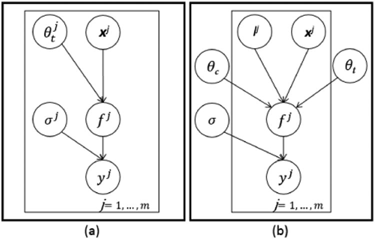
Graphical model for (a) m single-task Gaussian processes with m sets of: inputs Xⁱ, temporal covariance hyperparameters ${\theta }_t^i$, estimated functions fⁱ, noise terms σⁱ, and outcomes yⁱ; and (b) a multi-task Gaussian process which relates m tasks through all prior variables, with the tasks' labels l and similarity matrix θ_c.

Let ${\mathbf{X}}_{\mathbf{n}}=\{x_i^j|j=1,\dots ,m,i=1,\dots ,n_j\}$ and ${\mathbf{Y}}_{\mathbf{n}}=\{y_i^j|j=1,\dots ,m,i=1,\dots ,n_j,\}$ be the training indices and observations for the m tasks, where task j has n_j number of training data. We consider the regression model y⃗_n = g(x⃗_n) + ε, in which g(x) represents the latent function and $\epsilon \sim \mathcal{N}(0,{\sigma }_n^2)$ is a noise term. GP models assume that the function g(x⃗_n) can be interpreted as a probability distribution over functions such that ${\stackrel{\sim }{\mathbf{y}}}_{\mathbf{n}}=g({\overrightarrow{x}}_n)~\mathcal{G}\mathcal{P}(m({\overrightarrow{x}}_n),k({\overrightarrow{x}}_n,{\overrightarrow{x}}_n^{\prime }))$, where m(x⃗_n) is the mean function of the process (assumed = 0) and $k({\overrightarrow{x}}_n,{\overrightarrow{x}}_n^{\prime })$ is a covariance function describing the coupling among the independent variables x⃗_n as a function of their kernel distance. To specify the affiliation of index $x_i^j$ and observation $y_i^j$ to task j, a label l^j = j is added as an additional input to the model, as shown in Figure 1(b). To model the correlation between tasks as well as the temporal behaviour of the tasks within a unified GP model, two independent covariance functions are assumed, and the covariance matrix K_MT for all m tasks can be written

$${\mathbf{K}}_{MT}({\mathbf{X}}_n,\mathbf{l},{\mathit{\theta }}_c,{\mathit{\theta }}_t)={\mathbf{K}}_c(\mathbf{l},{\mathit{\theta }}_c)\otimes {\mathbf{K}}_t({\mathbf{X}}_n,{\mathit{\theta }}_t)$$ (1)

where ⊗ is the Kronecker product, l = {j | j = 1,…, m}, K_c and K_t represent the correlation and temporal covariance functions, and θ_c and θ_t are vectors containing hyperparameters for K_c and K_t, respectively. Within geostatistics, this approach is also known as the intrinsic correlation model (Wackernagel 2003).

By modifying the temporal covariance function we can encode our prior knowledge concerning the functional behavior of the tasks that we wish to model. The most frequently-used example is the squared-exponential covariance function (Rasmussen and Williams 2006):

$${\mathbf{K}}_t={\theta }_A^{2}exp\{-\frac{{\Vert x-x\prime \Vert }^2}{2{\theta }_L^2}\},$$ (2)

where θ_t = {θ_A, θ_L}, and θ_A and θ_L are hyperparameters modeling the y-scaling and x-scaling (or time-scale if the data are timeseries) of the covariance function, respectively.

To construct a valid positive semidefinite correlation covariance function K_c, we used the Cholesky decomposition and the “free-form” parameterization of the elements of the lower triangular matrix L proposed in (Bonilla, Chai, and Williams 2007), such as

$${\mathbf{K}}_c=\mathbf{L}{\mathbf{L}}^{\top },\mathbf{L}=\left[\begin{array}{cccc}{\theta }_{c,1}& 0& \cdots & 0\\ {\theta }_{c,2}& {\theta }_{c,3}& & 0\\ ⋮& & \ddots & ⋮\\ {\theta }_{c,k-m+2}& {\theta }_{c,k-m+2}& \cdots & {\theta }_{c,k}\end{array}\right]$$ (3)

where $k={\sum }_{i=1}^{m}i$ is the number of correlation hyperparameters.

Identically to STGPs, the hyperparameters θ for a MTGP may be optimized by minimizing the negative log marginal likelihood via gradient descent (Rasmussen and Williams 2006), and predictions for test indices $\{{\mathbf{x}}_p^{\ast },{\mathbf{l}}_p^{\ast }\}$ can be made by computing the conditional probability $p({\mathbf{y}}_p^{\ast }|{\mathbf{x}}_p^{\ast },{\mathbf{l}}_p,{\mathbf{x}}_n,{\mathbf{l}}_n,{\mathbf{y}}_n)$.

Figure 2 shows an example of STGPs and an MTGP applied to a simple synthetic dataset with 4 sample tasks. Tasks 1 and 2 were correlated, task 1 and task 2 were both anti-correlated with task 4, and task 3 was uncorrelated with all other tasks. For this, 4 tasks were sampled from a MTGP model with the following hyperparameters: θ_L = θ_A = θ_c,1 = θ_c,2 = θ_c,3 = θ_c,6 = θ_c,10 = 1, θ_c,4 = θ_c,5 = θ_c,0 = 0, and θ_c,7 = θ_c,8 = −1. Artificial gaps were then randomly created in different tasks at different time points and with different durations. The STGP (Figure 2(b)), applied to each task independently, fails to adequately represent the functions, particularly where data are not available. Figure 2(c) shows that the MTGP improves the predictions in all 4 tasks by capturing the relationships between them.

Figure 2.

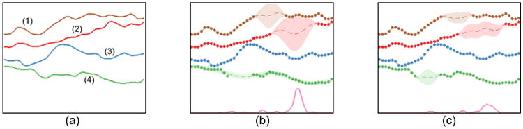
(a) A sample function with 4 tasks; (b) Single-task GP (STGP) and (c) multi-task GP (MTGP) predictions on all tasks. The dots represent observations, while dashed lines and colored areas represent the predictive mean and 95% confidence interval, respectively. The line on the bottom represents the mean absolute error (over the 4 tasks) between the predictions and the correspondent reference values. We observe that the overall error obtained in (c) is lower than that in (b), which suggests that the use of MTGP yielded better predictions by taking into account the correlation between the different tasks.

The MTGP has several useful properties as compared to the traditional GP:

• We can allow task-specific training indices n_j; i.e., training data may be observed at different times for different tasks (Figure 2);

• The correlations within and between tasks are automatically learned from the data by fitting the covariance function in Equation 1; and

• The framework assumes that the tasks have similar temporal characteristics and hyperparameters θ_t.

A limitation of the MTGP is computational cost: 𝒪(m³n³) compared with m × 𝒪(n³) for STGPs. This limitation is not as relevant for our application, given that we are not dealing with densely-sampled time-series data, but data which is sparse and irregular. Another limitation of the MTGP is that the number of hyperparameters can increase rapidly for an increasing number of tasks, which can lead to a multi-modal parameter space.

3.2 Signal Representation via Hyperparameters

We propose using the inferred MTGP hyperparameters θ that describe the temporal correlation within and between tasks as features that represent our set of observations: θ_A and θ_L which respectively govern each output scale of our functions and the input, or time, scale, and θ_c,i that correspond to the correlation between the different tasks (outputs) modelled. In effect, θ provides a new latent search space to examine and evaluate the similarity of any two given multidimensional functions. Importantly, these parameters are:

1. a means of representing the functional behavior a set of observations {y⃗_n, x⃗_n};

2. learned directly from data; and

3. generalizable to any type of longitudinal data, including categorical and numerical types.

4 Experiment 1: From Multiple Noisy Time-Series Data to Acuity Assessment

In this experiment, we use physiological signals from Traumatic Brain Injury (TBI) patients to test the MTGP's ability to assess and forecast multiple related signals. We examine two noisy timeseries: the intracranial pressure (ICP) and mean arterial blood pressure (ABP). Continuous monitoring of ICP and ABP has become a standard in neurological ICUs. Cerebrovascular autoregulation is an important mechanism to sustain adequate cerebral blood flow (Werner and Engelhard 2007), and impairment of this mechanism indicates an increased risk to secondary brain damage and mortality (Hlatky, Valadka, and Robertson 2005).

Cerebrovascular autoregulation is most commonly assessed based on the Pressure-Reactivity Index (PRx), which is defined as a sliding window Pearson's correlation between the ICP and ABP (Czosnyka et al. 1997). However, the ICP and ABP timeseries are often contaminated by artifacts and missing data, and PRx can no longer be calculated in these situations. Although methods have been proposed to detect and remove artifacts (Feng et al. 2011), the artifact removal process still creates gaps of missing data in the timeseries.

In this experiment, we demonstrate how the proposed MTGP model can be applied to interpolate the incomplete data in ICP and ABP signals and, more importantly, to accurately estimate PRx.

4.1 Data

The ICP and ABP data were collected from 35 TBI patients who were monitored for more than 24-hours in a Neuro-ICU of a tertiary care hospital between January 2009 and December 2010. The continuously monitored physiological readings were sampled and recorded every 10 seconds. For experimental evaluation, we selected 30 ten-minute windows from each patient recording, where ICP and ABP signals were free from artifacts and missing values. We then randomly introduced artificial gaps in both signals as shown in Figure 3. We evaluated the PRx estimation accuracy, and we further compared the performance of MTGP to that of STGP, which models each signal independently. For implementation, priors over the hyperparameters were selected after 100 random initializations for each case.

Figure 3.

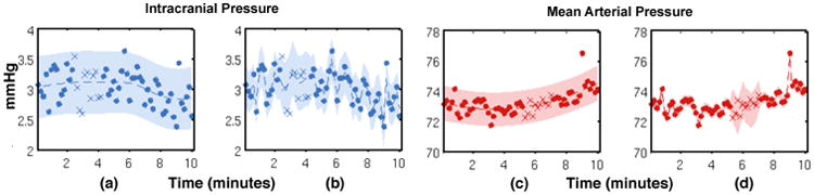
An example of a single-task GP (STGP) and multi-task GP (MTGP) applied to intracranial pressure (ICP) and mean arterial blood pressure (ABP) signals from a traumatic brain injury patient. (a) and (c) show the performance of STGP, whereas (b) and (d) show the improved performance of MTGP, which takes into account the correlation between ICP and ABP. Dots represent observations, crosses represent missing observations (test observations), the dotted line shows the function mean and the shaded area show the 95% confidence interval. We note that the timescale parameter “selected” by the MTGP, which takes into account the correlation between the tasks, is shorter than the one selected by the STGP, which yields to higher likelihood of the test observations (crosses).

4.2 Results

The quality of predictions are evaluated using the squared error loss, where we compute the squared residual (y* −ŷ*)² between the mean prediction (ŷ*) and the target (y*) at each test point, and the squared root of the average over the test set to produce the root mean squared error (RMSE). As the RMSE is sensitive to the overall scale of the target values, we additionally evaluate the negative log probability of the target under the model, by defining the mean standardized log loss (MSLL) as

$$\text{MSLL}(\widehat{\mathbf{y}}\ast ,\mathbf{y}\ast )=\frac{1}{p}\sum _{i=1}^p(-logp({\widehat{y}}_i^{\ast }|f,x_i^{\ast })+logp({\widehat{y}}_i^{\ast }|m({\mathbf{y}}_n),\text{var}({\mathbf{y}}_n),x_i^{\ast }),$$

where the first term is the log likelihood of ${\widehat{y}}_i^{\ast }$ given our latent function f and the test index $x_i^{\ast }$. This probability is normalized by the second term, the log likelihood of ${\widehat{y}}_i^{\ast }$ under a trivial model that predicts using a Gaussian with mean m(y_n) and variance var(y_n) of the training labels.

Table 1 shows the overall performance of our approach. We note that the MTGP was able to estimate the correlation between the ICP and ABP signals – PRx – accurately even with incomplete data. The average RMSE between the true correlation coefficients and the MTGP estimated ones with the incomplete data was 0.09 (Table 1). This suggests that the posterior hyperparameter of MTGP, which measures the interactions between ICP and ABP, may be used as an index to model the cerebrovascular autoregulation mechanism and thus the risk of secondary brain injury.

Table 1.

Performance of single-task GP (STGP) and multitask GP (MTGP). PRx-PRx* refers to the difference between the reference PRx (Pearson correlation coefficient of ICP and ABP for a given window) and PRx*, the estimated PRx index (posterior MTGP hyperparameter that measures the interaction between the two tasks).

Signal	Measure	STGP	MTGP
ICP	RMSE	0.91	0.69
	MSLL	0.6	0.45
ABP	RMSE	2.77	1.98
	MSLL	0.65	0.55
PRx-PRx*	RMSE	-	0.09

We note that the scale of ICP values is normally between 1 to 20 mmHg, and the specific ICP value determines whether the achieved reduction in RMSE is clinically significant. If the ICP has already elevated to somewhere near 20 mmHg, any slight increase in ICP may result in secondary damage to the brain. In this case, even small reductions to RMSE are more desirable to guide the medical interventions.

We also observe that the MTGP provides a significant improvement in interpolating values for both signals, as the correlation between the two physiological variables is taken into account. Particularly, in periods of incomplete data (see Figure 3), the predictions are much more accurate compared to STGP. This shows that the proposed MTGP model can also be used for accurate interpolation and forecasting of ICP and ABP timeseries in the applications of advanced alarming and physiological trajectory analysis.

5 Experiment 2: From Heterogenous Clinical Data to ICU Acuity Forecasting

To demonstrate the effectiveness of the proposed MTGP model on features inferred from sparse, irregularly sampled timeseries, we applied MTGPs to clinical notes from the ICU for mortality prediction as summarized in Figure 4. Gold-standard clinical models typically use population-based acuity scores, such as SAPS-I (Le Gall et al. 1984), based on snapshots of the patient's status during their stay in the ICU. These scores are inherently limited because patient state (or severity of illness) constantly evolves.

Figure 4.

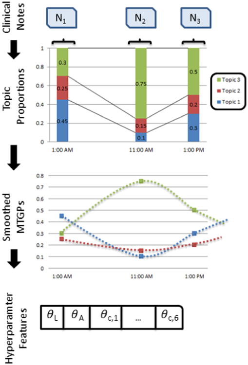
1) We perform a pre-projection step where clinical notes are transformed into timeseries using Latent Dirichlet Allocation; 2) the new set of topic proportion timeseries are fitted using the MTGPs; 3) inferred hyperparameters θ_L, θ_A, θ_c,1, …, θ_c,6 are derived, projecting into the new latent space; 4) latent features (hyperparameters) are used as features in combination with topic proportions and the SAPS acuity score to 5) forecast patient mortality.

5.1 Data

We used 2001–2006 ICU data from the open-access MIMIC II 2.6 database (Saeed et al. 2011), which includes electronic medical records (EMRs) for 26, 870 ICU patients at the Beth Israel Deaconess Medical Center (BIDMC).

For each patient we extracted the SAPS-I score, calculated from clinical variables over a patient's first 24-hours in the ICU. We used all notes from nursing, physicians, labs, and radiology recorded prior to the patient's first discharge from ICU. Discharge summaries were excluded because they typically state the patient's outcome explicitly. Patients were excluded if their notes had fewer than 100 words, fewer than 6 total notes in their record, or were under the age of 18. Patient mortality outcomes were measured at hospital discharge and 1 year post-discharge.

The final cohort consisted of 10,202 patients with 313,461 notes. A random 30% of the patients (3,040) were held back as a test set. The remaining 70% of patients (7,162) were used to train topic models and mortality predictors. The test set contained 93,411 notes, and the training set had 220,005.

5.2 Clinical Note Decomposition to Timeseries

Beginning from sparse, irregularly sampled clinical notes, we first performed topic modeling as a form of dimensionality reduction as described in (Ghassemi et al. 2014). Topics inference was performed on notes using T = 50 topics over the words (W) in our vocabulary (Blei, Ng, and Jordan 2003; Griffiths and Steyvers 2004). We normalized hyperparameters on the Dirichlet priors for the topic distributions (α) and the topic-word distributions (β) as $\alpha =\frac{50}{T}$, and $\beta =\frac{200}{W}$.

The topic inference resulted in a 50-dimensional vector of topic proportions for each note in every patient's record. We concatenated topic vectors into a matrix q where the element q_nk was the proportion of topic k in the n^th note.

5.3 Hyperparameter Construction

Once notes were transformed into multi-dimensional numeric vectors, we used the MTGPs to model the per-note change in topic membership over a patient's stay. This is critical for comparing two patients' records given that patients have different lengths of stay and note taking intervals depend on staff, clinical condition, and other factors.

From the topic enrichment measure (ϕ), we chose the topics with a posterior likelihood above or below 5% of the population baseline likelihood across topics. This yielded nine topics (see Table 5.3 for a summary of the chosen topics, and the Appendix for more details). We employed MTGP to learn the temporal correlation between the nine topics and the overall temporal variability of the multiple timeseries.

From the available data sources, we formed a set of three feature matrices: (1) the admitting SAPS-I score for every patient, (2) the average topic membership for the nine identified topics (matrix q), and (3) the inferred MTGP hyperparameters across the nine topic vectors from q. Importantly, the admitting SAPS-I score and mean topic members (1 and 2) are both static measures. SAPS-I collapses data from the first 24 hours of the record, while the average topic membership collapses the entire per-note timeseries for each patient's record into an aggregate measure. Our proposed MTGP hyperparameters (3) complement these measures with information about the per-note timeseries.

5.4 Outcome Classification

We considered five feature prediction regimes that combined subsets of the feature matrices 1, 2, and 3 as an aggregate feature matrix. We trained two supervised classifiers that were identical in the five feature sets used, but provided different objective functions for optimization: Lasso logistic regression and L2 linear kernel SVM.

Classifiers were trained to create classification boundaries for two clinical outcomes: in-hospital mortality and 1-year post-discharge mortality. All outcomes had large class-imbalance (e.g., in-hospital mortality rates of 10.9%). To address this issue, we randomly sub-sampled the negative class in the training set to produce a minimum 70%/30% ratio between the negative and positive classes. Test set distributions were not modified, and reported performance reflects those distributions. Due to space constraints, we only reported results on a completely held out test set. We performed 5-fold cross-validation on the remaining data, and cross-validation results were similar to those obtained on the completely held-out test set.

We evaluated the performance of all classifiers using the area under the Receiver Operating Characteristic curve (AUC) on the held-out test set. Table 3 reports results from the Lasso model. Results obtained using the L2 linear kernel SVM were not statistically different.

Table 3.

Prediction results of hospital and 1-year mortality, AUC for various feature combinations.

Features	Hospital Mortality	1-Year Mortality
SAPS-I	0.702	0.500
Ave. Topics	0.759	0.653
SAPS-I + MTGP	0.775	0.624
Ave. Topics + MTGP	0.788	0.673
SAPS-I + Ave. Topics + MTGP	0.812	0.686

5.5 Results

SAPS-I had the poorest predictive power, which is understandable given that it is only an initial snapshot (24 hours) of the severity of illness. We used the static SAPS-I score due to its status as the gold-standard in clinical scoring, and our argument in the second experiment is that the MTGP hyper-parameter space complements this clinical score, rather than competes with it. The average value of the most significant topics significantly improved upon that predictive power. The performance of MTGP Hyperparameters on their own was similar to that of the Topics: AUC of 0.749 and 0.624 for in-hospital and 1 year mortality, respectively.

Given that the hyperparameters were optimized from per-note topic features (that are themselves the output of an unstructured learning problem), it is most sensible that the topics information should be used in combination with the MTGP hyperparameters to describe patient state. We obtained improved predictive performance for both mortality outcomes when combining both MTGP hyperparameters with SAPS-I and the significant topics. This is likely because the hyperparameters provide complementary information to both SAPS-I and the significant topics. Both SAPS-I and the topic features capture a single aggregate measure of membership in certain latent dimensions related to outcome, while the MTGP hyperparameters capture movement over the course of a hospital stay within those dimensions. The best predictive performance occurred when all features were combined, e.g. SAPS-I + significant topics + MTGP hyperparameters.

6 Conclusion

The ability to determine on-going patient acuity has immediate clinical use. But clinical data are often noisy, sparse and irregularly sampled. The secondary nature of medical data is also true in other domains of application such as social media, online retailers, and online content distributors (e.g., Yelp reviews, Twitter tweets, Amazon product reviews and ratings). In all these cases, data are likely to suffer from the same problems mentioned above, but there is still a need to understand how sets of information are related. A key to analyzing such data is representing the time-series data in a manner that allows for effective discrimination between two or more patterns.

The goal of this work was to transform multiple clinical data sources (e.g., notes, acuity scores) into a new latent space where the information could be viewed as timeseries data, and abstracted features represent the series dynamics. We demonstrated our method's applicability to physiological and clinical data using two different experiments.

MTGPs were able to estimate the cerebrovascular autoregulation index in TBI patients. The biggest advantage of MTGP over STGP is the ability to estimate the correlations between ICP and MAP, even in the presence of missing data. This allows continuous assessment of the cerebral autoregulation mechanism, which is an important indicator of secondary brain damage and mortality.

Inferred MTGP hyperparameters were also able to increase classification performance on mortality prediction of ICU patients. The use of temporal information in clinical care is fundamental, and the large number of independent devices used in a modern ICU provides heterogeneous data. Using our method to summarize heterogenous clinical patient data into a more concise form, clinicians can leverage the collective knowledge of patient trajectories and outcomes. Concise representations of clinical notes are easier for clinicians to use, because they aggregate multi-author notes over time into topic timeseries that are more easily labeled (e.g. by viewing the top words) and tracked over a patient's record.

The main limitation in using this approach to characterize timeseries is computational cost. We conducted an exhaustive grid search over the constrained hyperparameter space. Computational costs may be addressed using a recently proposed Bayesian optimization for automatically tuning the MTGP hyperparameters (Swersky, Snoek, and Adams 2013) in large datasets. In a “real-time” setting, the computational cost for m tasks is O(m³, n³). An overview of sparse GP methods is presented in (Quionero-Candela and Rasmussen 2005), which aims to find a smaller set of pseudo-inputs n′ to reduce computational complexity. Further improvement is possible by 1) exploiting the Kronecker product (Stegle et al. 2011), 2) limiting the training data to the same time instances of each dimension of the data (Evgeniou, Micchelli, and Pontil 2005), or 3) by using recursive algorithms (Pillonetto, Dinuzzo, and De Nicolao 2010). Applications that require close-to-real-time retraining (e.g. Experiment 2), would benefit from these techniques, while operating over longer time-scales would be less sensitive.

Table 2.

Top five words in chosen topics (enriched for in-hospital mortality/survival).

	Top Five Words	Possible Topic
In-hospital Mortality	liver, renal, hepatic, ascites, dialysis	Renal Failure
	thick, secretions, vent, trach, resp	Respiratory infection
	remains, family, gtt, line, map	Systematic organ failure
	increased, temp, hr, pt, cc	Multiple physiological changes
	intubated, vent, ett, secretions, propofol	Respiratory failure
	name, family, neuro, care, noted	Discussion of end-of-life care
Survival	cabg, pain, ct, artery, coronary	Cardio-vascular surgery
	chest, pneumothorax, tube, reason, clip
	pain, co, denies, oriented, neuro	Responsive patient

References

- Blei D, Ng A, Jordan M. Latent dirichlet allocation. JMLR. 2003;3(5):993–1022. [Google Scholar]
- Bonilla EV, Chai KMA, Williams CK. Multitask gaussian process prediction. Advances in Neural Information Processing Systems. 2007:153–160. [Google Scholar]
- Breslow MJ, Badawi O. Severity scoring in the critically ill: Part 1interpretation and accuracy of outcome prediction scoring systems. CHEST Journal. 2012;141(1):245–252. doi: 10.1378/chest.11-0330. [DOI] [PubMed] [Google Scholar]
- Clifton D, Clifton L, Hugueny S, Wong D, Tarassenko L. An extreme function theory for novelty detection. Selected Topics in Signal Processing, IEEE Journal of. 2013a;7(1):28–37. [Google Scholar]
- Clifton L, Clifton D, Pimentel M, Watkinson P, Tarassenko L. Gaussian processes for personalized e-health monitoring with wearable sensors. Biomedical Engineering, IEEE Transactions on. 2013b;60(1):193–197. doi: 10.1109/TBME.2012.2208459. [DOI] [PubMed] [Google Scholar]
- Czosnyka M, Smielewski P, Kirkpatrick P, Laing R, Menon D, Pickard J. Continuous assessment of the cerebral vasomotor reactivity in head injury. Neurosurgery. 1997;41(1):11–17. doi: 10.1097/00006123-199707000-00005. [DOI] [PubMed] [Google Scholar]
- Durichen R, Pimentel M, Clifton L, Schweikard A, Clifton D. Multi-task gaussian processes for multivariate physiological time-series analysis. 2014 doi: 10.1109/TBME.2014.2351376. [DOI] [PubMed] [Google Scholar]
- Evgeniou T, Micchelli CA, Pontil M. Learning multiple tasks with kernel methods. Journal of Machine Learning Research. 2005 615637. 00441. [Google Scholar]
- Feng M, Loy L, Zhang F, Guan C. Conf Proc IEEE Eng Med Biol Soc. American Medical Informatics Association; 2011. Artifact removal for intracranial pressure monitoring signals: a robust solution with signal decomposition; pp. 797–801. [DOI] [PubMed] [Google Scholar]
- Fox EB, Sudderth EB, Jordan MI, Willsky AS. Joint modeling of multiple related time series via the beta process. arXiv preprint arXiv:1111. 2011;4226 [Google Scholar]
- Ghassemi M, Naumann T, Doshi-Velez F, Brimmer N, Joshi R, Rumshisky A, Szolovits P. Unfolding physiological state: Mortality modelling in intensive care units. 2014:75–84. doi: 10.1145/2623330.2623742. [DOI] [PMC free article] [PubMed] [Google Scholar]
- Griffiths T, Steyvers M. Finding scientific topics. PNAS. 2004;101:5228–5235. doi: 10.1073/pnas.0307752101. [DOI] [PMC free article] [PubMed] [Google Scholar]
- Hlatky R, Valadka AB, Robertson CS. Intracranial pressure response to induced hypertension: role of dynamic pressure autoregulation. Neurosurgery. 2005;57(5):917–923. doi: 10.1227/01.neu.0000180025.43747.fc. [DOI] [PubMed] [Google Scholar]
- Hug CW, Szolovits P. AMIA Annual Symposium Proceedings. Vol. 2009. American Medical Informatics Association; 2009. Icu acuity: real-time models versus daily models; p. 260. [PMC free article] [PubMed] [Google Scholar]
- Joshi R, Szolovits P. AMIA Annual Symposium Proceedings. Vol. 2012. American Medical Informatics Association; 2012. Prognostic physiology: Modeling patient severity in intensive care units using radial domain folding; p. 1276. [PMC free article] [PubMed] [Google Scholar]
- Lasko TA, Denny JC, Levy MA. Computational phenotype discovery using unsupervised feature learning over noisy, sparse, and irregular clinical data. PloS one. 2013;8(6):e66341. doi: 10.1371/journal.pone.0066341. [DOI] [PMC free article] [PubMed] [Google Scholar]
- Le Gall JR, Loirat P, Alperovitch A, Glaser P, Granthil C, Mathieu D, Mercier P, Thomas R, Villers D. A simplified acute physiology score for icu patients. Critical care medicine. 1984;12(11):975–977. doi: 10.1097/00003246-198411000-00012. [DOI] [PubMed] [Google Scholar]
- Lehman Lw, Saeed M, Long W, Lee J, Mark R. AMIA Annual Symposium Proceedings. Vol. 2012. American Medical Informatics Association; 2012. Risk stratification of icu patients using topic models inferred from unstructured progress notes; p. 505. [PMC free article] [PubMed] [Google Scholar]
- Li Q, Clifford G. Dynamic time warping and machine learning for signal quality assessment of pulsatile signals. Physiological Measurement. 2012;33(9):1491. doi: 10.1088/0967-3334/33/9/1491. [DOI] [PubMed] [Google Scholar]
- Lin J, Keogh E, Wei L, Lonardi S. Experiencing sax: a novel symbolic representation of time series. Data Mining and Knowledge Discovery. 2007;15(2):107–144. [Google Scholar]
- Marlin BM, Kale DC, Khemani RG, Wetzel RC. Proceedings of the 2nd ACM SIGHIT International Health Informatics Symposium. ACM; 2012. Unsupervised pattern discovery in electronic health care data using probabilistic clustering models; pp. 389–398. [Google Scholar]
- Pillonetto G, Dinuzzo F, De Nicolao G. Bayesian online multitask learning of gaussian processes. Pattern Analysis and Machine Intelligence, IEEE Transactions on. 2010;32(2) doi: 10.1109/TPAMI.2008.297. 193205. 00025. [DOI] [PubMed] [Google Scholar]
- Quionero-Candela J, Rasmussen CE. A unifying view of sparse approximate gaussian process regression. J Mach Learn Res. 2005;6:19391959. [Google Scholar]
- Rasmussen CE, Williams CKI. Gaussian Processes for Machine Learning (Adaptive Computation and Machine Learning) The MIT Press; 2006. [Google Scholar]
- Saeed M, Mark R. AMIA Annual Symposium Proceedings. Vol. 2006. American Medical Informatics Association; 2006. A novel method for the efficient retrieval of similar multiparameter physiologic time series using wavelet-based symbolic representations; p. 679. [PMC free article] [PubMed] [Google Scholar]
- Saeed M, Villarroel M, Reisner AT, Clifford G, Lehman LW, Moody G, Heldt T, Kyaw TH, Moody B, Mark RG. Multiparameter intelligent monitoring in intensive care ii (mimic-ii): a public-access intensive care unit database. Critical care medicine. 2011;39(5):952. doi: 10.1097/CCM.0b013e31820a92c6. [DOI] [PMC free article] [PubMed] [Google Scholar]
- Stegle O, Fallert S, MacKay DJC, Brage S. Gaussian process robust regression for noisy heart rate data. Biomedical Engineering, IEEE Transactions on. 2008;55(9):2143–2151. doi: 10.1109/TBME.2008.923118. [DOI] [PubMed] [Google Scholar]
- Stegle O, Lippert C, Mooij JM, Lawrence ND, Borgwardt KM. Efficient inference in matrix-variate gaussian models with$\backslash$ iid observation noise. Advances in Neural Information Processing Systems. 2011:630638. [Google Scholar]
- Swersky K, Snoek J, Adams RP. Multi-task bayesian optimization. Advances in Neural Information Processing Systems. 2013:2004–2012. [Google Scholar]
- Syed Z, Guttag JV. Unsupervised similarity-based risk stratification for cardiovascular events using long-term time-series data. Journal of Machine Learning Research. 2011;12:999–1024. [Google Scholar]
- Vincent JL. Critical care-where have we been and where are we going? Critical Care. 2013;17(Suppl 1):S2. doi: 10.1186/cc11500. [DOI] [PMC free article] [PubMed] [Google Scholar]
- Wackernagel H. Multivariate Geostatistics. Springer; 2003. [Google Scholar]
- Werner C, Engelhard K. Pathophysiology of traumatic brain injury. Br J Anaesth. 2007;99(1):4–9. doi: 10.1093/bja/aem131. [DOI] [PubMed] [Google Scholar]
Associated Data
This section collects any data citations, data availability statements, or supplementary materials included in this article.