Time-dependence of graph theory metrics in functional connectivity analysis

Abstract

Brain graphs provide a useful way to computationally model the network structure of the connectome, and this has led to increasing interest in the use of graph theory to quantitate and investigate the topological characteristics of the healthy brain and brain disorders on the network level. The majority of graph theory investigations of functional connectivity have relied on the assumption of temporal stationarity. However, recent evidence increasingly suggests that functional connectivity fluctuates over the length of the scan. In this study, we investigate the stationarity of brain network topology using a Bayesian hidden Markov model (HMM) approach that estimates the dynamic structure of graph theoretical measures of whole-brain functional connectivity. In addition to extracting the stationary distribution and transition probabilities of commonly employed graph theory measures, we propose two estimators of temporal stationarity: the S-index and N-index. These indexes can be used to quantify different aspects of the temporal stationarity of graph theory measures. We apply the method and proposed estimators to resting-state functional MRI data from healthy controls and patients with temporal lobe epilepsy. Our analysis shows that several graph theory measures, including small-world index, global integration measures, and betweenness centrality, may exhibit greater stationarity over time and therefore be more robust. Additionally, we demonstrate that accounting for subject-level differences in the level of temporal stationarity of network topology may increase discriminatory power in discriminating between disease states. Our results confirm and extend findings from other studies regarding the dynamic nature of functional connectivity, and suggest that using statistical models which explicitly account for the dynamic nature of functional connectivity in graph theory analyses may improve the sensitivity of investigations and consistency across investigations.

1. Introduction

Connectomic analysis using graph theoretical methods is increasingly found to be a powerful quantitative method for investigating complex brain networks on the whole-brain level. Through the computation of neurobiologically interpretable network measures, graph theory provides a mathematical framework through which topological properties of the network may be studied, including aspects related to clustering, efficiency, modularity, long-range connectivity, and small-worldness [1, 2]. Its application to functional data on resting state networks from functional MRI, magnetoencephalography, and electroencephalography has provided novel insights into various neurological and psychiatric diseases [3, 4, 5, 6]. Increasingly, studies are demonstrating the utility of graph theory measures of functional connectivity for identifying abnormalities in network connectivity and serving as clinical diagnostic markers and as markers of disease severity [7, 8, 9, 10].

Despite the large number of analyses of resting-state network connectivity that use graph theory to explore network connectivity, the majority rely on the assumption of temporal stationarity. In most cases, the strength of inter-regional signal associations is calculated using some measure of linear dependence, such as the synchronization likelihood or a measure of correlation, over the entire scanning session. The strength of these associations is then either analyzed as weighted graphs or binarized into unweighted graphs [2]. However, recent evidence increasingly shows that inter-regional signal associations are dynamic over time, and are highly modulated by attention, medications, and cognitive state [11]. In addition, [12] have found that resting state functional connectivity exhibits a large degree of variability both within and across scanning sessions. [13] have also demonstrated that functional connectivity fluctuates over time within scans, furthermore finding that first-order temporal dynamics may approximate these dynamics. Although the reasoning behind the dynamic nature of resting-state brain topology is a relatively new concept and under investigation, it is thought to reflect the configuration of functional networks around a stable anatomical skeleton [14]. Computational modeling and empirical work have demonstrated that, at shorter time scales, these various functional network configurations may be spontaneously visited around the same anatomical skeleton in the presence of local cell dynamics [14]. While some aspects of brain topology, such as the level of small-worldness, may exhibit greater temporal stationarity in order to maintain a relatively constant optimum network configuration, others, such as local measures, may be more susceptible to local cell dynamics and more likely to traverse multiple configurations. Various functional configurations may also exist in order to allow flexibility to support different cognitive functions [15].

Recently, studies have noted that conflicting results have arisen in graph theory investigations of functional connectivity. Investigations of clustering coefficient and characteristic path length, for example, have variably found evidence of increase, decrease, or no change in patients with epilepsy compared to controls [6, 16]. One contributing factor to current inconsistencies in the literature may be small sample sizes and moderate effect sizes [16]. In light of recent evidence that resting-state functional connectivity is in fact non-stationary, however, another major factor may be greater temporal instability in some topological characteristics than others, leading some investigations to capture the topology of particular functional network configurations while other investigations may capture other topological configurations. Understanding of temporal dynamics of graph measures of network topology may help address these previous literature inconsistencies.

The aim of this study is to identify which aspects of network topology exhibit less within-scan temporal variability in resting state networks, with the objective of evaluating which graph theory metrics may be robustly estimated using static functional connectivity analyses. To the best of our knowledge, this is the first attempt of quantifying the relative temporal stationarity of graph theory metrics of brain network topology in functional connectivity analysis. In particular, we use a Bayesian hidden Markov model to estimate the transition probabilities of various graph theoretical network measures using resting-state fMRI (rs-fMRI) data. We propose two estimators of temporal stationarity, which can be used to quantitate different aspects of the temporal stationarity of functional networks: the N-index, which is a deterministically-based estimator of the number of change-points, and the S-index, which is a probabilistically-based estimator that takes into account stochastic variation in the estimated states. Based on the estimated stationarity distribution and transition probabilities, we evaluate the relative levels of temporal stationarity among various commonly investigated measures of brain network topology. Additionally, we point to possible hierarchical extensions of our model which may be used to aid in disease prediction, by showing that incorporating temporal dynamics into investigations of brain connectivity may increase discriminatory power of graph theory metrics.

2. Materials and Methods

In order to determine which aspects of network topology are robust under static functional connectivity analysis, we investigate commonly employed graph theoretic measures in current literature using a Bayesian hidden Markov model. We apply our proposed estimators to the healthy control and temporal lobe epilepsy populations, and illustrate that differences in temporal dynamics between epileptic and healthy brain networks may be quantitated and may provide a potential diagnostic marker.

2.1. Participants

Participants consisted of 24 healthy controls (HC; average age, 32.50 ± 1.88 SE (y); range/Q₁/Q₃, 19-64/27/35 (y); 8 females) and 32 patients with temporal lobe epilepsy (TLE; average age, 37.56±1.86 SE (y); range/Q₁/Q₃, 20-63/32/45 (y); 16 females; average epilepsy duration, 18.79 ± 2.25 SE (y); range/Q₁/Q₃, 2-45/6/31 (y)). Healthy control subjects had normal structural MRIs and no history of neurologic illness or were taking neurologic medications. TLE patients were recruited from the University of California, Los Angeles (UCLA) Seizure Disorder Center. Diagnostic evaluation for all subjects included video-EEG monitoring, high-resolution MRI, FDG-PET scanning, and neuropsychological testing. Written informed consent was obtained prior to scanning for all subjects in accordance with guidelines from the UCLA Institutional Review Board. A two-sample t-test with unequal variances and Fisher exact test showed no significant difference in age or gender, respectively at the α=0.05 level of significance.

2.2. Image acquisition and pre-processing

Imaging was performed with a 3T MRI system (Siemens Trio, Erlangen, Germany). Functional imaging was performed with the following parameters: TR=2000 ms, TE=30 ms, FOV=210 mm, matrix= 64 × 64, slice thickness 4 mm, 34 slices. Subjects were instructed to relax with eyes closed during imaging. No auditory stimulus was present except for the acoustic noise from imaging. High-resolution structural images were obtained during the same imaging study with the parameters: TR=20 ms, TE=3 ms, FOV = 256 mm, matrix = 256 × 256, slice thickness 1 mm, 160 slices. The images were acquired in the axial plane using a spoiled gradient recalled (SPGR) sequence for the anatomical images and an echo planar imaging (EPI) sequence for the functional images. The imaging sessions included multiple simultaneous EEG and fMRI recordings, each lasting 5 to 15 minutes. For resting state fMRI analysis, 20 minutes of BOLD fMRI data was used for each subject. To limit the influences of motion, subjects were checked to ensure that no subjects had a maximum translation of > 1.5mm (HC, 0.24 ± 0.04 mm; TLE, 0.37 ± 0.04 mm). Resting-state fMRI was performed for TLE patients after the comprehensive epilepsy surgery evaluation and prior to epilepsy surgery. Patients remained on their regular medications during the fMRI. None of the patients had a seizure in the 24 hours preceding the imaging. None of the patients had seizures during the study as confirmed by the simultaneous EEG obtained during fMRI. The EEG results were not included in the data analysis other than to exclude seizures. Details of the simultaneous EEG methods have been described previously [17]. Neuroimaging and fMRI pre-processing steps are similar to that described previously [18]. Preprocessing was performed using FSL (fMRIB Software Library) version 5.0.7 (Oxford, United Kingdom, www.fmrib.ox.ac.uk/fsl) [19, 20] and included head movement artifact correction [21], nonbrain tissue elimination [22], high-pass filtering (100 s), spatial smoothing at 5 mm full-width half-maximum, and mean-based intensity normalization as described previously for resting-state fMRI analyses [23, 24]. Excessive head movement was corrected using motion scrubbing through nuisance regression [25]. We used the tool fsl motion outliers within FSL to identify TRs that showed instantaneous changes in blood oxygen level-dependent (BOLD) intensity that exceeded threshold (75th percentile + 1.5× interquartile range). The average number of identified outliers per participant was 4.11%±2.65%. Tissue-type segmentation was performed on each participant's structural image using FAST (FMRIB's Automated Segmentation Tool) [26], before being aligned to their respective BOLD images. White matter signal and cerebrospinal fluid signals were obtained using the segmented masks. The following were included as temporal covariates and regressed out using linear regression: motion outliers, six motion parameters, white matter signal, cerebrospinal fluid signal, and their associated derivatives. The residuals were then filtered through a low pass filter (< 0.1 Hz).

2.3. Functional network construction and graph theory metrics

Functional BOLD images were segmented into 90 regions of interest using the automated anatomical labeling (AAL) atlas. Each BOLD image was registered to the participant's high-resolution structural image using FLIRT (FMRIB's Linear Image Registration Tool) [21, 27, 28], and the high-resolution structural was registered to the standard MNI space using FNIRT (FMRIB's Non-linear Image Registration Tool) [29]. The transformation matrix and warpfields were inverted, and then applied to the 90 regions of interest to obtain ROI masks in each individual's BOLD space. Functional connectivity between each pair of nodes was computed as the Pearson correlation between the average regional time series, using a sliding-window approach. A window size of 44s were used with 50% overlap to segment the original 300 volumes in each region into 26 windows. The effect of window size has been investigated in [30], with a window size of 44s found to provide a good trade-off between the quality of covariance matrix estimation and resolution of functional dynamics. [31] found that cognitive states can be correctly identified with as few as 30 – 60s of data, with topological assessments estimated to stabilize for window lengths greater than 30s [32]. Variation in window size between 30s and 2 minutes has been found to have little effect on functional dynamics [30]. Negative correlations were set to zero to improve the reliability of graph theory measures [33]. Binary undirected graphs were constructed by thresholding the correlation matrix across a series of biologically plausible network densities [2], yielding a range of potential undirected graphs of the brain's functional network. This procedure ensured that between-network and between-group comparisons of graph theory metrics reflected differences in topological organization rather than differences in absolute connectivity. This resulted in a non-random connection density range of 0.37 – 0.50, in order to involve graphs that were fully connected for all windows for all subjects (degree > 1 for all nodes) and non-random topological properties [34]. Network measures were averaged across the non-random connection density range, with the same range used in order to ensure comparability between populations.

In this study, we investigate network characteristics related to small-world index (σ), global integration (λ, normalized characteristic path length; GE, global efficiency), local segregation (γ, normalized clustering coefficient; LE, average local efficiency), and centrality (BC, betweenness centrality; EC, eigenvector centrality). A vast number of graph theory measures of network topology have been recently studied in various neurological diseases. The majority of these features relate to various aspects of global network integration or local segregation [35, 36, 37]. Another important subset of features identifies nodes that have a strong influence on the communication of the network, which are known as centrality or hub measures. The simplest of these centrality measures is degree centrality, which counts the number of edges connected to each node. Other centrality measures capture more nuanced quantities, such as eigenvector centrality, which identifies nodes that are connected to other highly central nodes, or betweenness centrality, which captures the number of shortest paths that pass through a node [38]. In addition, presence of deviations from a small-world configuration has been consistently found to characterize various types of brain disease, including Alzheimer's disease, epilepsy, brain tumors, and traumatic brain injury [3]. Graph theory measures were calculated as in [1] using the Brain Connectivity Toolbox in Matlab version R2014b. Normalization of characteristic path length and clustering coefficient was relative to a set of 500 randomly rewired graphs [39].

2.4. Bayesian hidden Markov model

A hidden Markov model is a state-space model with discrete hidden states, which is able to capture sequential dependence structure in the data. Indeed, HMMs have been successfully employed in the analysis of data with such intrinsic structure, see [40] and [41] for examples on array comparative genomic hybridization (CGH) data, and [13] for a frequentist application on spatial functional connectivity.

We model the time-varying aspect of graph theory metrics by treating the observed value of the graph theory metric as the realization of a time-varying hidden state, which we denote ξ_it. Let $X_{it}^{(g)}$ denote the value of graph theory metric g (g = 1, …, G), for subject i (i = 1, …, n) during time t (t = 1, …, T). For each time point $t=1,\dots ,T,X_{it}^{(g)}$ is obtained by computing the graph metric g on sliding windows centered at time t. For simplicity, in the below we omit the index g.

From a mathematical point of view, a HMM comprises of two components: a Markov chain with stochastic measurements on the hidden states and, conditionally on the states, an independent emission distribution (Figure 1). In the context of our specific application, we choose a first-order HMM on the latent functional connectivity states. This choice assumes that the probability of being in a specific hidden state at a specific time point depends only on the hidden state at the previous time point, as described in formula by

Figure 1.

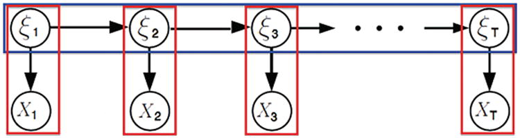
A hidden Markov model consists of a Markov chain with stochastic measurements on the hidden states (ξ₁, …, ξ_T) and an independent emission distribution (X₁, …, X_T) conditional on the states.

$$P({\xi }_{it}|{\xi }_{i1},\dots ,{\xi }_{i(t-1)})=P({\xi }_{it}|{\xi }_{i(t-1)})=a_{{\xi }_{i(t-1)}{\xi }_{it}},$$ (1)

where A = (a_hj) is a matrix of transition probabilities whose elements a_hj indicate the transition probability from state h to state j. The transition matrix A has a unique stationary distribution π_A = (π_A(1), …, π_A(K)) for states k = 1, …, K. We assume that the state of the first time point is distributed as π_A. As for the emission distribution, we assume that, conditional on the hidden states, the observed graph theory metric values are independent and follow a distribution with state-specific parameters θ_j,

$$X_{it}|{\xi }_{it}=j~f(X_{it};{\mathit{\theta }}_j)$$ (2)

where for graph theory metrics with support (−∞, ∞) we define $f(X_{it};{\mathit{\theta }}_j)=\mathrm{N}({\mu }_j,{\sigma }_j^2)$. As discussed by [42], this density can be used to approximate any finite continuous density function arbitrarily closely. Therefore, the full likelihood can be factorized as

$$L(X|\xi =j)=\prod _{i=1}^n\prod _{t=1}^{T}f(X_{it};{\theta }_j).$$ (3)

Pulling together the likelihood in Equation 3 and the Markov chain in Equation 1, the first-order HMM employed can be described by the following factorization:

$$P({\mathit{X}}_1,\dots ,{\mathit{X}}_T,{\mathit{\xi }}_1,\dots ,{\mathit{\xi }}_T)=\prod _{i=1}^{n}L(X_{i1}|{\xi }_{i1})P({\xi }_{i1})\prod _{t=2}^{T}L(X_{it}|{\xi }_{it})P({\xi }_{it}|{\xi }_{i(t-1)}).$$ (4)

As for the prior specification of our modeling approach, we assume conjugate independent Dirichlet priors on the rows of the transition probability matrix

$${\mathit{a}}_h~\text{Dir}({\alpha }_1,\dots ,{\alpha }_K),$$

where K is the number of states. We further place conjugate vague priors on the parameters of the emission distributions:

$$\begin{array}{l}p({\mu }_j)=\mathrm{N}({\delta }_j,{\tau }_j^2)\hfill \\ p({\sigma }_j^2)=\text{IG}(c_j,d_j)\hfill \end{array}$$

∀j = 1, …, K. Note that here and throughout this paper IG denotes the Inverse-Gamma distribution. Employing conjugate vague priors is a common choice in the Bayesian literature to approximate non-informative priors in the absence of prior information, following their introduction by [43].

2.4.1. MCMC algorithm and posterior inference

The joint posterior distribution of all parameters of interest can be sampled employing a Metropolis-within-Gibbs sampling technique. This combines Metropolis-Hastings steps as proposed by [41] for updating the transition probability matrix and state matrix with Gibbs steps for sampling the mean and variance of the hidden states conditional upon the other parameters. Full details of the full conditional distributions and MCMC implementation are provided in Appendix A. Given the MCMC output, we perform inference on the states, ξ, by calculating, for each ξ_it, the maximum a posteriori estimate using the mode of the state values after burn-in. Posterior inference on the transition matrix and emission parameters is performed through the posterior mean to minimize squared error loss.

In our analysis, all hyperparameters were set to be non-informative, with δ_j = 0 and α_j = 1 ∀j. Data were standardized through centering and scaling prior to usage in the Gaussian emission distribution. Therefore, we expect 99.7% of the data to fall within three standard deviations of the mean. Consequently, we set the prior variance of the state means, τ_j, to ${\left(\frac{X_{(n)}-X_{(1)}}{6}\right)}^2$, where X_(n) and X₍₁₎ are, respectively, the maximum and minimum values observed in the data. As for the shape and scale hyperparameters of the state-specific variances c_j and d_j, we set these to yield a prior expectation of 0.5 and prior variance of 2 on the distribution of ${\sigma }_j^2$. The MCMC chain was initialized with initial values ${\sigma }_j^{(0)}=1$ and ${\mu }_j^{(0)}$ set to equally spaced intervals from [−1, 1] ∀j. We initialized ξ⁽⁰⁾ by setting ${\xi }_{it}^{(0)}=j$ if the corresponding T_j < X_it < T_j+1, where $\mathit{T}=[-\infty ,\frac{1}{K},\frac{2}{K},\dots ,\frac{K-1}{K},\infty ]$. We initialized A⁽⁰⁾ from the initial value of ξ⁽⁰⁾, by setting $a_{hj}^{(0)}$ to the proportion of transitions from state h to state j in ξ⁽⁰⁾. For each measure, we ran 50,000 MCMC iterations with the first 30,000 sweeps discarded as burn-in.

All code was written in R version 3.1.3. A software package to carry out implementation has been made available at the corresponding author's website [Note to editor: Software will be made available upon publication]. Code is available upon request from the corresponding author.

2.5. Statistical inference on relative temporal stationarity of graph theory metrics

We propose two estimators of the relative temporal stationarity of each graph theory metric: the N-index, which is a deterministically-based estimator of the number of change-points, and the S-index, which is a probabilistically-based estimator that takes into account stochastic variation in the estimated states. To our knowledge, although some investigation into general aspects of temporal stationarity in functional connectivity has shown that functional connectivity fluctuates over time [13, 30], no attempt has yet been made to provide quantitative estimates of the temporal stationarity of specific aspects of graph topology. Furthermore, we allow for direct comparison of relative temporal stationarity across measures or across disease populations by proposing scalar indexes of stationarity. The first estimator, the N-index, estimates the proportion of time that the network measure spends in stable states (i.e., not in change-points). Importantly, we show that our proposed estimator is an unbiased and asymptotically consistent estimator of the average proportion of time spent in stable states. The second estimator, the S-index, provides a weighted estimate of the stationarity of the dominant state, and takes into account probabilistic variation of the hidden states.

1. N-index: This is proposed as the complement of the mean proportion of change-points, where the number of change-points for a given subject is estimated based on the posterior mode of posterior samples of ξ, i.e.

   $$N=1-\frac{1}{n(T-1)}\sum _{i=1}^n\sum _{t=2}^T{\mathbf{1}}_{\{{\widehat{\xi }}_{it}\ne {\widehat{\xi }}_{i(t-1)}\}}$$ (5)

   where ξ̂_it denotes the posterior mode across the posterior samples of ξ_it ∀i, t. Due to estimation based on the posterior mode of ξ, the N-index yields a deterministic estimator of the general stationarity of the process. As shown in Appendix B, (5) provides an unbiased and asymptotically consistent estimator of the average proportion of time spent in a stable state. Similarly, for inference on the individual subject level, (5) reduces to:

   $$N_i=1-\frac{1}{T-1}\sum _{t=2}^T{\mathbf{1}}_{\{{\widehat{\xi }}_{it}\ne {\widehat{\xi }}_{i(t-1)}\}}.$$
2. S-index: The second estimator, the S-index, is proposed as the weighted mean of the probabilities of remaining in the same state from time t to time t + 1, where weights are given by the stationary distribution, i.e.

   $$S=\sum _{j=1}^K{\widehat{\pi }}_j{\widehat{a}}_{jj}$$ (6)

   where π̂ = (π̂_j) is the posterior mean of the stationary distribution, and â_jj denotes the jth diagonal element of the posterior mean of the estimated transition probability matrix, Â. In contrast to the N- index, we propose the S index solely for inference on the group level. In addition, whereas the N-index is based on deterministically estimated states, the S-index is a probabilistic estimator which takes into account the stochastic variation of the estimated states through (6). The definition in (6) allows S to assume values in the interval [0, 1]. The estimated S-index approaches 1 if the probability of staying in the same state goes to 1, while the estimated S-index approaches 0 if the probability of transitioning to a different state goes to 1. By weighting the probabilities by the stationary distribution, larger weight is assigned to states which occur more frequently in the process. Thus, if the probability of remaining in a given state is small for state j, but the graph theory metric spends little time in state j, then less weight is given to this probability in computing (6). Conversely, if the probability of remaining in a given state is small for state j, and the graph theory metric spends a large proportion of time in state j, then more weight is given to this probability in computing (6).

Whereas the N-index measures the frequency of change-points, the S-index takes into account both the frequency of change-points as well as whether the network measure has a dominant state or exists in multiple states more equally. A network measure which has a low-frequency of change-points as well as exists in a dominant state will result in a high N-index and high S-index.

2.6. Model validation

The proposed method was tested on simulated data for n = 30 subjects and T = 300 time points. Model performance in accurately predicting the transition probability matrix and hidden states was validated using the mean square error and misclassification error. Model validation is shown in Appendix C.

2.7. Temporal dynamics and class separability

Our model provides a hierarchical modeling approach to estimating temporal non-stationarity, which may be built upon to aid diagnostic prediction. In particular, the likelihood in (2) may be extended to a discriminant analysis context, allowing for probabilistic prediction of disease status. Here, we illustrate the potential utility of individual differences in the temporal dynamics of graph measures to increase discriminatory power. To obtain a measure of the increase in discriminatory power after accounting for temporal dynamics for various graph measures, we evaluated two criteria for class separability. The first separation criterion is based on the well-known ratio of the within-class scatter matrix and between-class scatter matrix, known as the Fisher criterion:

$$J=\text{tr}({\sum }_W^{-1}{\sum }_B),$$ (7)

where Σ_B is the between-class scatter matrix and Σ_W is the within-class scatter matrix. Larger values of J generally indicate greater class separability, based on a larger between-class scatter relative to within-class scatter. However, because the separability criterion in (7) is not directly related to classification error [44], we adopted a second measure, the Bhattacharyya distance, defined as:

$$BD=\frac{1}{8}{({\mu }_1-{\mu }_2)}^T{\left[\frac{{\sum }_1+{\sum }_2}{2}\right]}^{-1}({\mu }_1-{\mu }_2)+\frac{1}{2}ln\frac{|({\sum }_1+{\sum }_2)/2|}{{|{\sum }_1|}^{1/2}{|{\sum }_2|}^{1/2}}$$

where μ_i, Σ_i are the mean and covariance of class i, respectively. As shown by [45], BD is a class separability measure that yields the upper and lower bounds of Bayes classification error, with higher values of BD yielding lower levels of classification error. Class separability was assessed for three feature combinations: (1) the estimated graph metric under the assumption of stationarity, (2) the N-index of the graph metric, and (3) the combined feature vector of the estimated graph metric and corresponding N-index.

3. Results

3.1. Model comparison

The model and proposed estimators were applied to two neurologic populations of interest studied in brain connectivity research, the healthy control and temporal lobe epilepsy populations. For each network measure, we explore HMM fits over a grid of values of K (K = 2, …, 6 in our study) to find the number of states K yielding the best model fit. Model fit for each value of K was assessed using the deviance information criterion (DIC) and convergence of the state allocations to the stationary distribution. Models with lower DIC indicate better goodness of fit and are generally preferable to models with higher DIC. The DIC for each model is shown in Figure 2. In our study, state allocations showed convergence to a unique stationary distribution for K = 2. For K > 2 states, trace plots for the following graph measures: BC (HC, TLE), σ (HC, TLE), λ (HC, TLE), GE (HC), EC (HC), and γ (TLE) appeared to switch between a few local optima, following a behavior consistent with the artificial splitting of a single state into multiple states [46]. For γ (HC), LE (HC, TLE), and EC (TLE), DIC was minimized for an HMM fit with K = 2 states. For GE (TLE), DIC was minimized for an HMM fit with K = 3 states.

Figure 2.

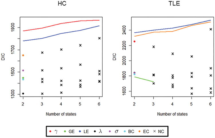
Model fitting: DIC for different values of K. γ, clustering coefficient; GE, global efficiency; LE, local efficiency; λ, path length; σ, small-world index; BC, betweenness centrality; EC, eigenvector centrality; NC, non-convergent solution. Crosses indicate non-convergent solutions.

3.2. Relative temporal stationarity of graph metrics

The relative temporal stationarity of the different network measures among healthy controls and TLE patients based on estimated values of N-index and S-index is shown in Figure 3(a) and (b), respectively. Posterior probabilities of the relative levels of temporal stationarity were estimated through Monte Carlo approximation and are shown in Table E.1. Among healthy controls, small-world index was consistently identified by both the N-index and S-index to exhibit the greatest temporal stationarity among network measures (Figure 3(a)-(b), Table E.1). Global efficiency exhibited greater temporal stationarity than local efficiency, while betweenness centrality exhibited greater stationarity than eigenvector centrality. For global integration measures, global efficiency exhibited greater stationarity than characteristic path length. The estimated stationary distribution for each network measure, which provides the equilibrium probability that the Markov chain is found in each particular state, describes the expected long-run behavior of the chain and is shown in Figure 4. Among healthy controls, local segregation measures (γ, LE) and eigenvector centrality demonstrated the least amount of evidence for existence of a single dominant state, spending roughly equal amounts of time in each state. In contrast, global integration measures (λ, GE), small-world index, and betweenness centrality each demonstrated greater evidence for existence of a dominant state, with greater than 0.70 probability of being found in a single dominant state for each of these measures (Figure 4).

Figure 3.

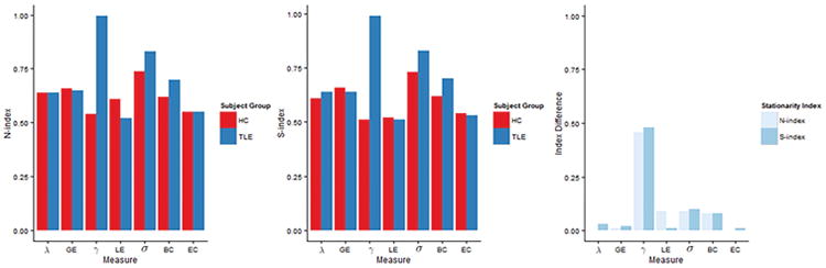
Temporal stationarity of graph metrics of (a) healthy controls and TLE patients using N-index and (b) healthy controls and TLE patients using S-index. In (c), magnitude of differences in temporal stationarity between healthy controls and TLE patients for the various graph metrics are shown.

Figure 4.

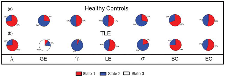
Pie chart showing stationary distribution of (a) healthy controls; and (b) TLE patients. λ, normalized characteristic path length; GE, global efficiency; γ, normalized clustering coefficient; LE, local efficiency; σ, small-world index; BC, betweenness centrality; EC, eigenvector centrality.

TLE patients exhibited similar patterns in the relative temporal stationarity of each network measure, with two primary exceptions. Firstly, TLE patients exhibited weaker evidence for a difference between global efficiency and path length than healthy controls (Table E.1). The second exception was with respect to clustering coefficient for TLE patients, which was consistently identified as one of the least temporally stationary network measures for healthy controls but to exhibit great temporal stationarity for TLE patients (Figure 3). Consistent with this observation, the stationary distribution of clustering coefficient for TLE patients estimated that more than 90% of the scan was spent in a single dominant state for clustering coefficient (Figure 4). Global integration measures (λ, GE), small-world index, and betweenness centrality each were expected in the long-run to have greater than 0.70 probability of being found in a single dominant state in TLE patients. Three-state and two-state models for global efficiency among TLE patients were similar with respect to the long-run proportion of time spent in the dominant state (Figure F.1).

3.3. Temporal dynamics and class separability

Here, we explore the potential diagnostic utility of incorporating temporal dynamics into graph theory estimates. Figure 3(c) shows the magnitude of the difference in S-index and N-index between TLE and controls, for various graph theory measures. Overall, the S-index and N-index identified consistent differences in the temporal stationarity of network measures between TLE patients and healthy controls, with minor differences due to the probabilistic versus deterministic nature of the estimators. Clustering coefficient demonstrated the largest difference in the level of temporal stationarity between healthy controls and TLE patients. Small-world index and betweenness centrality also demonstrated moderate differences in the level of temporal stationarity between disease and normal brain states (Figure 3(c)). Differences between TLE patients and healthy controls based on the N-index of clustering coefficient, small-world index, and betweenness centrality are shown in Figure 5(a). The ability of the N-index to capture individual differences in temporal stationarity is shown for a few representative subjects in Figure G.1 (Appendix G). In particular, we see the group differences apparent in Figure 5(a) reflected on the individual subject level in Figure G.1. From Figure 5(a), the N-index of clustering coefficient, small-world index, and betweenness centrality was generally higher in TLE compared to controls, with the greatest difference present in clustering coefficient. This is apparent in Figure G.1 on the individual subject level, as a lower frequency of change-points and longer stretches of stationarity among TLE patients than in healthy controls.

Figure 5.

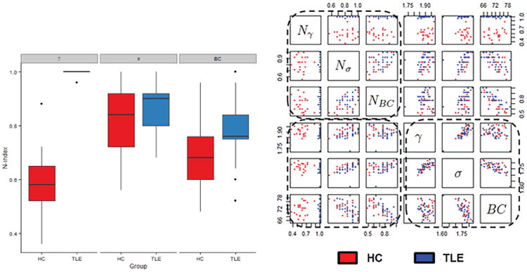
(a) Boxplots showing the estimated N-index for clustering coefficient (γ), small-world index (σ), and betweenness centrality (BC) for healthy controls and TLE patients. (b) Scatterplots showing the separation of pathological states based on the graph metric alone (bottom right panel); N-index alone (upper left panel); and combination of the N-index and graph metric (bottom left panel). We note that when temporal dynamics are considered as an additional feature, the pathological states exhibit much greater separability.

Class separability for each graph measure, as well as the corresponding N-index of temporal stationarity, is shown in Table 1(a)-(b) and (d)-(e), respectively. Table 1(c) and (f) shows the class separability when the N-index of the graph measure was used as a feature in addition to the estimated graph measure. We observed that the Fisher criterion and Bhattacharyya distance yielded similar results, with increased class separability observed between TLE and controls when temporal stationarity was taken into account. In particular, the Fisher criterion for class separability was greater when the N-index was considered as an additional feature along with the estimated graph metric for both clustering coefficient and small-world index (Table 1). This indicates a greater level of between-class relative to within-class scatter when the N-index was considered as an individual feature. The Bhattacharyya distance between the classes increased as well for clustering coefficient, small-world index, and betweenness centrality when the N-index was considered as an individual feature, indicating better separability between the classes. Although the Fisher criterion failed to identify an increase in class separability for betweenness centrality when the N-index was taken into account, this may reflect the closeness of the centroids of the respective classes to the overall centroid.

Table 1.

Class separability based on Fisher criterion for (a) graph metric, (b) N-index, and (c) graph metric + N-index; and based on Bhattacharyya distance for (d) graph metric, (e) N-index, and (f) graph metric + N-index. γ, clustering coefficient; σ, small-world index; BC, betweenness centrality.

	Fisher criterion			Bhattacharyya distance
	(a)	(b)	(c)	(d)	(e)	(f)
γ	0.0440	8.0700	5.9309	0.0356	4.2482	4.4366
σ	0.0193	0.0658	0.0614	0.0357	0.0414	0.2111
BC	0.0060	0.1475	0.0062	0.00508	0.0745	0.1661

The added contribution of the N-index to the original graph metric in diagnostic prediction is visualized in Figure 5(b). The bottom right panel of Figure 5(b) demonstrates the difficulty of differentiating the pathological classes when considered only with respect to the whole-brain graph metrics. When temporal dynamics are considered, the pathological states exhibit much greater separability (bottom left, top left panels).

4. Discussion

In this study, we investigate the temporal stationarity of various graph theoretical measures of network topology from resting-state fMRI data. We propose two quantitative scalar estimators of temporal stationarity, the S-index and N-index, which may be used to compare different aspects of temporal stationarity across disease populations or across network measures, while allowing for different levels of probabilistic uncertainty through the two estimators. Our quantification of the temporal stationarity of topological characteristics related to small-world index, global integration, local segregation, and centrality provides, to our knowledge, the first attempt to understand the temporal dynamics of different aspects of brain network topology. We show that several graph theoretical measures, including small-world index, global integration measures, and betweenness centrality, may be more robust to an assumption of temporal stationarity in functional connectivity analyses than others. In addition, we demonstrate that subject-level differences in the temporal stationarity of network topology may be useful as an additional marker of abnormality.

4.1. Graph measures and temporal stationarity

Functional connections can be roughly classified into two categories: long-range connections between different modules or clusters of neurons, and local connections within modules or clusters of neurons. While the former allows for integration of different sources of information, the latter allows for local information processing [47]. Network measures of global integration were observed here to generally exhibit greater stationarity than network measures of local segregation. This may reflect the organization of the resting-state brain, in which the small-world architecture of the brain is thought to have evolved in order to create systems that support efficiency in both local and global processing [48]. Since long-range connections are generally thought to ensure the interaction between distant neuronal clusters [47], a large component of fluctuations between neuronal clusters (e.g., long-range connections) may therefore occur downstream to fluctuations within neuronal clusters (e.g., local connections), resulting in slightly greater temporal stationarity among global relative to local connections. Furthermore, while connectivity within local subgraphs may be more susceptible to local cell dynamics and likely to fluctuate over time, higher levels of local fluctuations may be expected to be associated with lower levels of long-range fluctuations in order to maintain relatively constant net levels of temporal variability. Although the concept of the brain network as a closed system has been discussed previously [48], its potential impact on the temporal dynamics of network topology remains relatively unknown.

Small-world index was observed to be one of the topological network measures exhibiting the greatest amount of stationarity on the seconds time scale among healthy controls. This is perhaps unsurprising, as small-world index provides a measure of the level of optimality of the network structure for synchronizing neural activity between brain regions [49, 50] as well as efficient information exchange [48], and may be thus less likely to be affected over short increments of time analyzed within a single scanning session. It may also be of interest to note that the level of small-worldness of a network is based on the ratio of clustering coefficient to characteristic path length. Therefore, the fact that small-world index consistently exhibited greater levels of temporal stationarity than both clustering coefficient and characteristic path length among healthy controls indicates that clustering coefficient and characteristic path length tended to fluctuate in the same direction among healthy controls. In contrast, small-world index among TLE patients consistently exhibited greater levels of temporal stationarity than characteristic path length, but lower levels of stationarity than clustering coefficient. This indicates that there was a lower correspondence between the tendency of clustering coefficient and characteristic path length to fluctuate in the same direction among TLE patients. [51] suggested that an optimal balance between global integration and local segregation, reflected by the level of small-worldness, is needed to support efficient information processing. It may be that dynamic increases (decreases) in local segregation are normally accompanied by increases (decreases) in global integration in order to maintain an optimal level balance of network integration and segregation in the healthy control population. Our results suggest that the temporal correspondence between network integration and segregation may be affected in pathology.

Among global integration measures, we found that global efficiency exhibited greater temporal stationarity than characteristic path length with high posterior probability among healthy controls. In contrast, only weak evidence was present for such a relationship among TLE patients. While global efficiency is the average inverse shortest distance between two generic nodes in the network and is a measure of parallel efficiency, characteristic path length is the average shortest distance between two generic nodes and a measure of sequential efficiency [48]. Our observation that global efficiency exhibits greater temporal stationarity than characteristic path length, therefore, suggests that the level of parallel efficiency of brain networks remains more constant over time than the level of sequential efficiency. A similar phenomenon is observed in computer system design, in which parallel computing systems exhibit greater fault tolerance than sequential computing systems, due to the redundancy and ability for error checking and correction provided by parallel compared to sequential streams [52]. Our interesting observation confirms the similarity of construction principles among brain and other networks.

4.2. Implications for inter-study replicability and temporal lobe epilepsy

The differences in temporal stationarity between different topological characteristics identified here, with some measures tending to remain in a single state than others, may be one reason underlying the inconsistencies between existing studies regarding the direction in which topological characteristics are altered in disease. Here, we found that clustering coefficient demonstrates the least amount of evidence of the existence of a single dominant state in the healthy control population, as quantified by its estimated stationary distribution, and moreover spent the largest proportion of time in change-points, as quantified through the N-index and S-index. Several review studies have, in fact, observed that case-control studies investigating how clustering coefficient is altered in disease using static connectivity analyses have resulted in inconsistent conclusions. In temporal lobe epilepsy, for example, [6] found that there exists a large amount of variation in conclusions regarding the direction of alteration of clustering coefficient in temporal lobe epilepsy relative to healthy controls, with both increases [53, 54, 55, 56] and decreases [5, 57, 58] identified. [59] also observed inconsistencies across studies which have evaluated the directionality of altered clustering coefficient among Alzheimer's disease relative to healthy controls, with both increases [60] and decreases [10] identified. Inconsistencies have generally been attributed to differences in imaging modalities, analytic methods, or clinical heterogeneity between studies. The temporal non-stationarity of clustering coefficient among healthy controls found in our study, however, suggests that another reason for current between-study inconsistencies may relate to the lack of temporal stationarity of clustering coefficient. In particular, some studies may capture clustering coefficient of their healthy control sample in one particular state, whereas other studies may capture clustering coefficient in another state. If this is the case, then utilization of statistical methods which account for the dynamic nature of connectivity, rather than assuming temporal stationarity, may be appropriate to attain better estimated values of clustering coefficient. Betweenness centrality was also consistently more temporally stable than eigenvector centrality across models in both TLE and healthy subjects. The higher level of temporal stationarity of betweenness centrality may lead to a higher level of sensitivity in characterizing hub distributions based on static analytic approaches. Betweenness centrality has been consistently implicated in both localizing [7] and lateralizing TLE [61, 62], whereas eigenvector centrality has been less well implicated.

Notably clustering coefficient, while the least stable measure among healthy controls, was the most temporally stable measure among TLE patients, surpassing even small-world index in temporal stationarity. We postulate that this may relate to neuronal cell loss secondary to seizures in TLE. A meta-analysis of focal epilepsies, for example, found that the focal epileptic brain has a more segregated and less integrated network [16]. This implies that nodes become more tightly interconnected with immediate neighbors and less connected with nodes outside their immediate neighborhood, with a more densely connected neighborhood facilitating more stable local connections in TLE.

The proposed measures of temporal stationarity in this study facilitate future exploration of the ability of temporal stationarity levels of different network measures to serve as diagnostic biomarkers. Here, we found that considering the N-index of graph metrics in addition to their estimated values may significantly increase the discriminant power of classifiers between TLE patients and healthy controls. Future investigation is needed in order to further evaluate the feature importance of these measures for prediction of diagnostic and prognostic status.

4.3. Limitations

As mentioned in the Results section, the proposed model requires the number of states in the HMM to be fixed a priori. We found that two or three states optimally maximized the goodness of fit for whole-brain graph theory metrics in our sample of temporal lobe epilepsy patients and healthy controls. A separate study on the dynamics of whole-brain functional connectivity in schizophrenic patients and healthy controls also found that three states optimally maximized the difference between within- and between-cluster variance [13]. Another study on young healthy controls found that seven states optimally characterized whole-brain functional connectivity dynamics [30]. A third study also found that generalizability in healthy controls drastically decreases after six or seven states, and that gains in generalizability are generally reduced after three or four states in simulated data [63]. The number of states K in the HMM is not generalizable across populations and data types, and K should be optimized for each individual dataset. In HMMs, there have generally been two approaches employed for choosing the number of states K. The first approach is the one we have employed, in which K is fixed a priori. The HMM model is fit over a grid of values of K, and the model fit for each value of K is then assessed through a goodness-of-fit criterion, such as the deviance information criterion [64]. The second approach uses Bayesian non-parametrics [65, 66], which has the advantage of automatically learning the value of K but the disadvantage of the need to explore transdimensional parameter spaces, thus adding to the computational demands of the algorithm.

A practical issue in using HMMs is that the estimation of state-specific parameters is subject to sample size constraints. The primary algorithmic stability concern that arises as the number of states increases is that a lower number of observations are expected to be assigned to a specific state. This is equivalent of reducing the sample size for the estimation of the transition matrix, the vector of state-specific means, and the vector of state-specific variances. Therefore, the number of estimable free parameters is constrained by the number of time points and samples. Another computational concern is that the DIC must be computed for each number of states. However, as each model is independent of the other, computational speed-up may be attained through parallel processing.

4.4. Future work

The results presented in this work suggests several lines of future research. Firstly, we used the Pearson correlation coefficient to estimate functional connectivity between nodes. Although this is the predominant method that has been used to estimate undirected graphs in current resting-state fMRI studies, several other methods exist to estimate undirected graphs, including graphical lasso [67], partial correlation coefficients, and a large number of other possible methods for quantifying associations. Each of these methods provides an approximation to the true unknown graphical structure of the brain, and future studies may wish to evaluate whether some topological measures exhibit greater temporal stationarity under some estimation procedures than others. Whether temporal stationarity may also be improved through usage of particular parcellation schemes or variations in graph theory metric calculation should also be explored. Secondly, in order to facilitate comparison with current graph theory investigations, graph metrics for each window were estimated by averaging over the non-random connection density range, as the coefficient of variation across thresholds for each graph measure was within the range of within-subject variability described for fMRI data [68]. A straightforward extension of our model which avoids this averaging step is to directly model the vector within the emission distribution. Thirdly, we examined connectivity using a sliding window approach with a window size of 44s and 50% overlap. This choice was based on previous studies, which have found that a shorter window size of 44s provides the ability to resolve temporal dynamics while providing a good tradeoff with the quality of covariance matrix estimation [30]. Varying window size between 30s and 2 minutes has been found to have relatively little impact on functional connectivity dynamics other than the expected result of reducing the variability associated with longer time windows [30]. Lastly, to identify dynamic patterns of graph theoretical measures, we used a finite HMM with Gaussian emission distribution. Although HMMs are an efficient way of recovering complex Markov processes in which hidden states emit the observed data according to some probability distribution, they have several limitations including difficulty separating heavily overlapped states. Of note, the overall higher DIC in TLE patients suggests that the temporal dynamics of brain topology in TLE patients may be more complex than in healthy controls, which may be captured by additional model parameters. Several extensions of the hierarchical model proposed in this paper may be explored to improve inference, including the use of Bayesian non-parametric methods to avoid a priori specification of the number of states, or different emission distributions in the HMM to accommodate graph theory measures with integer support spaces. Inference may also benefit from a larger number of time points and the inclusion of additional subjects.

Highlights.

• Temporal stationarity of graph theory measures of functional connectivity are examined.

• A Bayesian hidden Markov model is proposed to estimate temporal transitions.

• Two estimators of temporal stationarity are proposed to capture different levels of probabilistic uncertainty.

• Small-world index, global integration measures, and betweenness centrality exhibit greater temporal stationarity.

• Differences in temporal stationarity may aid in disease group discrimination.

Appendix A. MCMC algorithm

We employ Markov chain Monte Carlo (MCMC) methods to sample from the joint posterior distribution of {A, ξ, θ_j}. In particular, at iteration (s):

1. Update A with Metropolis-Hastings step:

   Propose $a_h^{\mathit{\text{new}}}~\text{Dir}({\alpha }_1+o_{h1},\dots ,{\alpha }_K+o_{hK})$ where $o_{hj}={\sum }_{i=1}^n{\sum }_{t=1}^{T-1}{\mathbf{1}}_{\{{\xi }_{it}=h,{\xi }_{i(t+1)}=j\}}$, j = 1, …, K, for all rows h. Jointly accept $A^{\mathit{\text{new}}}=(a_1^{\mathit{\text{new}}},\dots ,a_K^{\mathit{\text{new}}})$with probability

   $$min[1,\prod _{i=1}^n\frac{{\pi }_{A^{\mathit{\text{new}}}}({\xi }_{i1})}{{\pi }_{A^{\mathit{\text{old}}}}({\xi }_{i1})}].$$
2. Update $\underset{n\times T}{\underbrace{\xi }}$ with Metropolis-Hastings step. For each column t = 1, …, T:

   1. For each element ξ_it, i = 1, …, n: If t = 1, propose ${\xi }_{i1}^{\mathit{\text{new}}}~\text{Cat}({\pi }_{A^{(s)}})$. If t > 1, propose ${\xi }_{it}^{\mathit{\text{new}}}$ from the current transition probability matrix A^(s), i.e.

      $$p({\xi }_{it}^{\mathit{\text{new}}}=j|{\xi }_{i(t-1)}^{(s-1)}=h)=a_{hj}^{(s)}\forall i=1,\dots ,n_t.$$
   2. For each element ξ_it, i = 1, …, n_t, accept ${\xi }_{it}^{\mathit{\text{new}}}$ with probability

      $$min[\frac{p(X|{\mathit{\xi }}^{\mathit{\text{new}}})p({\mathit{\xi }}^{\mathit{\text{new}}})q({\mathit{\xi }}^{\mathit{\text{old}}}|{\xi }^{\mathit{\text{new}}})}{p(X|{\mathit{\xi }}^{\mathit{\text{old}}})p({\mathit{\xi }}^{\mathit{\text{old}}})q({\mathit{\xi }}^{\mathit{\text{new}}}|{\xi }^{\mathit{\text{old}}})},1]$$

      where

      $$\frac{p(X|{\mathit{\xi }}^{\mathit{\text{new}}})}{p(X|{\mathit{\xi }}^{\mathit{\text{old}}})}\propto \frac{f(X_{it};{\theta }_j,{\xi }_{it}^{\mathit{\text{new}}})}{f(X_{it};{\theta }_j,{\xi }_{it}^{\mathit{\text{old}}})}$$

      and where

      $$\begin{array}{l}\frac{p({\mathit{\xi }}^{\mathit{\text{new}}})q({\mathit{\xi }}^{\mathit{\text{old}}}|{\xi }^{\mathit{\text{new}}})}{p({\mathit{\xi }}^{\mathit{\text{old}}})q({\mathit{\xi }}^{\mathit{\text{new}}}|{\xi }^{\mathit{\text{old}}})}=\frac{p({\mathit{\xi }}^{\mathit{\text{new}}}|{\mathit{\xi }}^{\mathit{\text{new}}})q({\mathit{\xi }}^{\mathit{\text{old}}}|{\xi }^{\mathit{\text{new}}})}{p({\mathit{\xi }}^{\mathit{\text{old}}}|{\mathit{\xi }}^{\mathit{\text{old}}})q({\mathit{\xi }}^{\mathit{\text{new}}}|{\xi }^{\mathit{\text{old}}})}\\ \propto \frac{{\prod }_{i=1}^{n}p({\xi }_{i(t+1)}^{\mathit{\text{old}}}|{\xi }_{it}^{\mathit{\text{new}}})p({\xi }_{it}^{\mathit{\text{new}}}|{\xi }_{i(t-1)}^{\mathit{\text{old}}})}{{\prod }_{i=1}^{n}p({\xi }_{i(t+1)}^{\mathit{\text{old}}}|{\xi }_{it}^{\mathit{\text{old}}})p({\xi }_{it}^{\mathit{\text{old}}}|{\xi }_{i(t-1)}^{\mathit{\text{old}}})}\cdot \frac{{\prod }_{i=1}^{n}q({\xi }_{it}^{\mathit{\text{old}}}|{\xi }_{i(t-1)}^{\mathit{\text{old}}})}{{\prod }_{i=1}^{n}q({\xi }_{it}^{\mathit{\text{new}}}|{\xi }_{i(t-1)}^{\mathit{\text{old}}})}\\ =\frac{{\prod }_{i=1}^{n}p({\xi }_{i(t+1)}^{\mathit{\text{old}}}|{\xi }_{it}^{\mathit{\text{new}}})}{{\prod }_{i=1}^{n}p({\xi }_{i(t+1)}^{\mathit{\text{old}}}|{\xi }_{it}^{\mathit{\text{old}}})}\\ \propto \frac{p({\xi }_{i(t+1)}^{\mathit{\text{old}}}|{\xi }_{it}^{\mathit{\text{new}}})}{p({\xi }_{i(t+1)}^{\mathit{\text{old}}}|{\xi }_{it}^{\mathit{\text{old}}})}\end{array}$$ (A.1)

      and where all transition probabilities in (A.1) are as given in the current transition probability matrix A^(s). Note that (A.1) is true for every t < T, while for t = T the ratio simplifies to 1.
3. Update parameters of emission distributions:

   1. Update μ_j, j = 1, …, K with Gibbs step: Draw

      $${\mu }_j|\cdot ~\mathrm{N}(\frac{[{\sum }_{i=1}^n{\sum }_{t=1}^T{X}_{it}{\mathbf{1}}_{\{{\xi }_{it}=j\}}]/{\sigma }_j^2+{\delta }_j/{\tau }_j^2}{(n_j)/{\sigma }_j^2+1/{\tau }_j^2},\frac{1}{(n_j)/{\sigma }_j^2+1/{\tau }_j^2})$$

      ∀j = 1, …, K, where $n_j={\sum }_{i=1}^n{\sum }_{t=1}^T{\mathbf{1}}_{\{{\xi }_{it}=j\}}$.
   2. Update ${\sigma }_j^2$, j =, …, K with Gibbs step: Draw

      $${\sigma }_j^2|\cdot ~\text{IG}(\frac{n_j}{2}+c_j,\frac{1}{2}\sum _{i=1}^n\sum _{t=1}^T{(X_{it}-{\mu }_j)}^2{\mathbf{1}}_{\{{\xi }_{it}=j\}}+d_j)$$

      ∀j = 1, …, K, where $n_j={\sum }_{i=1}^n{\sum }_{t=1}^T{\mathbf{1}}_{\{{\xi }_{it}=j\}}$.

4. Due to the invariance of the likelihood in (3) under permutations of the labels of the hidden states, label-switching occurs in hidden Markov models. We account for label-switching by enforcing the identifiability constraint μ₁ < μ₂ < … < μ_k. In particular, we permute the values of ξ and θ_j on-line to satisfy the above constraint.

Appendix B. Proof of unbiasedness and asymptotic consistency of N-index

It can be shown that (5) is an unbiased estimator of the average proportion of time spent in a stable state. In order to do so, it is enough to show that

$$\mathbb{E}[N]=\mathbb{E}[1-\frac{1}{n(T-1)}\sum _{i=1}^n\sum _{t=2}^T{\mathbf{1}}_{\{{\widehat{\xi }}_{it}\ne {\widehat{\xi }}_{i(t-1)}\}}]=1-\frac{1}{n(T-1)}\sum _{i=1}^n\sum _{t=2}^T\mathbb{E}[{\mathbf{1}}_{\{{\widehat{\xi }}_{it}\ne {\widehat{\xi }}_{i(t-1)}\}}]=1-\frac{1}{n(T-1)}\sum _{i=1}^n\sum _{t=2}^T\mathbb{P}[{\widehat{\xi }}_{it}\ne {\widehat{\xi }}_{i(t-1)}].$$

Furthermore, the variance of (5) asymptotically goes to 0 as either the number of subjects n → ∞ or the number of time points T → ∞, since

$$Var[N]=Var[1-\frac{1}{n(T-1)}\sum _{i=1}^n\sum _{t=2}^T{\mathbf{1}}_{\{{\widehat{\xi }}_{it}\ne {\widehat{\xi }}_{i(t-1)}\}}]=\frac{1}{n^2{(T-1)}^2}\sum _{i=1}^n\sum _{t=2}^{T}Var[{\mathbf{1}}_{\{{\widehat{\xi }}_{it}\ne {\widehat{\xi }}_{i(t-1)}\}}]=\frac{1}{n^2{(T-1)}^2}\sum _{i=1}^n\sum _{t=2}^T\mathbb{P}[{\xi }_{it}\ne {\xi }_{i(t-1)}](1-\mathbb{P}[{\xi }_{it}\ne {\xi }_{i(t-1)}])$$ (B.1)

which clearly goes to 0, since $\frac{1}{n^2{(T-1)}^2}\to 0$ faster than the summand goes to ∞. Note that the independence of indicators in (B.1) follows from first-order Markov property.

Appendix C. Evaluation of performance using simulated data

Here, we evaluate the performance of the model through simulated data, and demonstrate the utility of our proposed stationarity measures, the N-index and S-index, for quantifying aspects of temporal stationarity.

Appendix C.1. Simulation settings

In this section, we use simulated data to evaluate the performance of the Bayesian hidden Markov model for identifying hidden states and transition probabilities for graph theory metrics. In order to assess performance of the model in accurately estimating transition probabilities, we compute the mean square error of the estimated transition probabilities. We assess performance in accurately predicting the hidden states by computing the misclassification error for the estimated hidden state matrix, ξ. In addition, we demonstrate the utility of the N-index and S-index as quantitative measures for capturing the frequency of transitions between states.

In particular, we simulate data on graph theory metrics for n = 30 subjects and T = 300 time points. Using the silhouette index [69], three states has been found to optimally maximize the difference between within- and between-cluster variation for the strength of functional connections [13]. For each graph theory network measure, these three states are ordered, lending to a natural interpretation of these states as characterizing low, normal, and high levels of each network measure. Transitions between adjacent ordered states are expected to be more likely than transitions between non-adjacent ordered states (e.g., low levels of network connectivity, for example, are more likely to transition to a normal level of network connectivity before progressing to a high level of network connectivity). Based on these considerations, we generate the simulated n × T matrix ξ of hidden states as follows:

1. Using the following transition probability matrix:

   $$\left[\begin{array}{ccc}.75& .18& .07\\ .49& .002& .508\\ .01& .40& .59\end{array}\right]$$ (C.1)

   we follow [40] and [41], and sample the first column (i.e., the hidden states of the n samples at the first time point) from the initial probability vector π_A, which is calculated as the normalized left eigenvector associated with the principal eigenvalue.

2. Given the first column of ξ, we sample all other columns from the transition probability matrix in (C.1).

Given ξ, we generate simulated values of X as in (2), where we fix μ₁ = −0.5, μ₂ = 0, μ₃ = 0.5, σ₁ = σ₂ = σ₃ = 0.1. The simulated data are shown in Figure C.1 (left) and the underlying transition matrix is shown in Figure C.2 (left). Hidden states are shown in Figure C.2 (right). To evaluate robustness of our model to different levels of overlap between the states, we also evaluate a second scenario, with μ₁ = −0.3, μ₂ = 0, μ₃ = 0.3, σ₁ = σ₂ = σ₃ = 0.1 (Figure C.1, right).

Hyperparameters were set to be non-informative when possible. In particular, we set δ_j = 0, τ_j = 100, c_j = 2, d_j = 1 ∀j, α₁ = α₂ = α₃ = 1. The MCMC chain was initialized with initial values ${\mu }_1^{(0)}=-1$, ${\mu }_2^{(0)}=0$, ${\mu }_3^{(0)}=1$, and ${\sigma }_1^{(0)}={\sigma }_2^{(0)}={\sigma }_3^{(0)}=1$. We initialized ξ⁽⁰⁾ by setting ${\xi }_{it}^{(0)}=j$ if the corresponding T_j < X_it < T_j+1, where T = [−∞, −0.5, 0.3, ∞] for the first scenario, and T = [−∞, −0.2, 0.2, ∞] for the second scenario. We initialized A⁽⁰⁾ from the initial value of ξ⁽⁰⁾, by setting $a_{hj}^{(0)}$ to the proportion of transitions from state h to state j in ξ⁽⁰⁾. We ran 1000 iterations with the first 500 sweeps discarded as burn-in. Convergence to the stationary distribution was assessed using the Raftery-Lewis diagnostic.

Figure C.1.

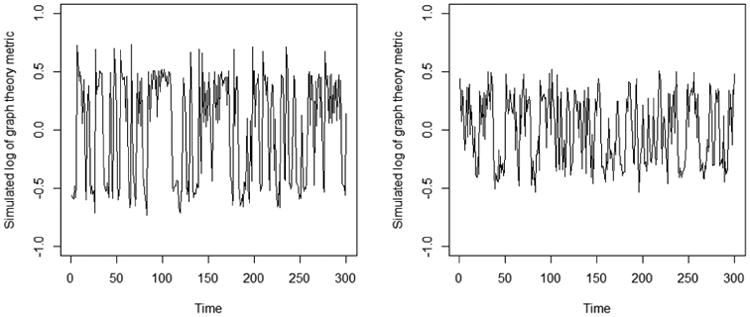
Simulated data: (Left) Simulated values of graph theory metric (μ₁ = −0.5, μ₂ = 0, μ₃ = 0.5) and (Right) Simulated values of graph theory metric (μ₁ = −0.3, μ₂ = 0, μ₃ = 0.3), for a sample subject.

Appendix C.2. Performance on simulated data

Figure C.2 (a) shows the performance of our model for estimating the transition probability matrix and graph theory states under the first scenario. Performance under the second scenario, with a greater amount of overlap between the states, is shown in Figure C.2 (b). Predicted values of the transition probabilities were close to the true transition probabilities, with a mean square error of 0.0013 under the first scenario, and a mean square error of 0.0009 under the second scenario. Hidden states were also predicted with high accuracy for both small and large levels of overlap between the states, with a misclassification error of 0.23% for the first scenario, and a misclassification error of 4.76% for the second scenario.

Other parameters of interest, including the stationary distribution and measures of temporal stationarity, can also be inferred upon. In the first scenario, the stationary distribution, π̂, was estimated from the normalized left eigenvector of the predicted transition probability matrix as π̂ = [0.446 0.205 0.349]. In other words, the subject would be expected in the long-run to spend 44.5% of time in State 1, 34.9% of time in State 3, and 20.5% of time in State 2. The N-index was estimated as 0.553, indicating that an estimated 55.3% of the time was spent in stable states. The S-index was estimated on the scale of [0, 1] as 0.554, indicating that the weighted probability of only 0.554 for remaining in same state. As seen from Figure C.2 (a) and Figure C.2 (b), the proposed S-index appears to provide a good quantitative measure of the temporal stationarity of the dominant states, as frequent transitions are observed to occur for this graph theory metric between states 1 and 3. Estimates of the stationary distribution and stationarity of graph theory metric remained robust under higher levels of overlap between the states, with an estimated stationary distribution of π̂ = [0.445 0.213 0.342], estimated N-index of 0.566, and estimated S-index of 0.543 under the scenario of μ₁ = −0.3, μ₂ = 0, μ₃ = 0.3.

Figure C.2.

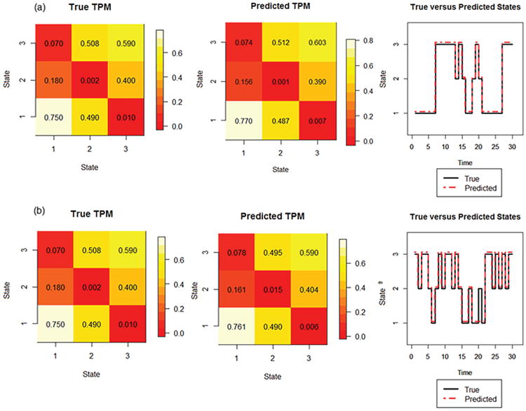
Simulated data. (a) μ₁ = −0.5, μ₂ = 0, μ₃ = 0.5: (Left) True transition probability matrix, (Middle) Posterior mean estimated transition probability matrix, (Right) True and posterior mode of predicted states for a sample subject. (b) μ₁ = −0.3, μ₂ = 0, μ₃ = 0.3: (Left) True transition probability matrix, (Middle) Posterior mean estimated transition probability matrix, (Right) True and posterior mode of predicted states for a sample subject. For true and predicted states, first 30 time points shown are shown for simplicity.

Appendix D. Supplementary material for Section 3.1

Figure D.1.

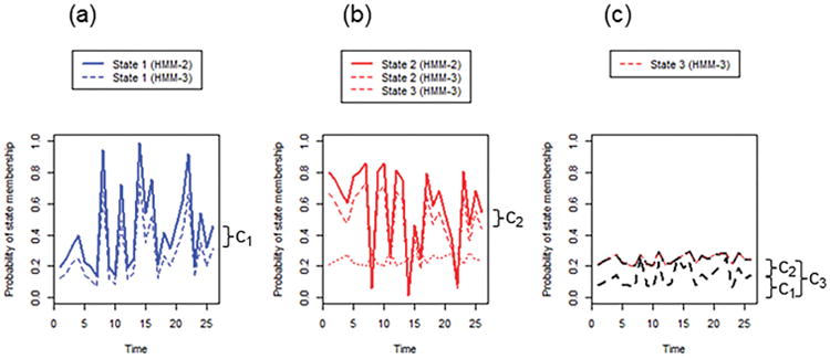
Example of model fitting in the event of mis-specification. Estimated probabilities of belonging to each state at each time point is shown for eigenvector centrality of a given subject. (A) The probability of belonging to State 1 under the 3-state HMM is approximately equal to the probability of belonging to State 1 under the 2-state HMM, minus a small constant c₁. (B) The probability of belonging to State 2 under the 2-state HMM is approximately equal to the probability of belonging to State 2 under the 3-state HMM, plus a small constant c₂. The probability of belonging to State 3 under the 3-state HMM, c₃, is composed of c₁ and c₂, and is small compared to the peaks in A and B.

Appendix E. Estimates of posterior probability of relative levels of temporal stationarity

Table E.1.

Posterior probabilities of relative temporal stationarity for graph metrics. (a) Posterior probability of greater temporal stationarity in global efficiency than in path length; (b) posterior probability of greater temporal stationarity in betweenness centrality than in eigenvector centrality; (c) posterior probability of greater temporal stationarity in global efficiency than in local efficiency; (d) posterior probability of greater temporal stationarity in small-world index than in the other graph measures. λ, characteristic path length; GE, global efficiency; γ, clustering coefficient; LE, local efficiency; σ, small-world index; BC, betweenness centrality; EC, eigenvector centrality.

	HC		TLE
(a) Global integration measures (GE vs. λ)
	NGE > Nλ	SGE > Sλ	NGE > Nλ	SGE > Sλ
	0.81	0.78	0.54	0.52
(b) Centrality measures (BC vs. EC)
	NBC > NEC	SBC > SEC	NBC >NEC	SBC > SEC
	0.90	0.87	0.994	0.993
(c) Efficiency measures (GE vs. LE)
	NGE >NLE	SGE > SLE	NGE > NLE	SGE > SLE
	0.98	0.97	0.97	0.96
(d) Small-world index
	Nσ > NZ	Sσ > SZ	Nσ > NZ	Sσ > SZ
Z = γ	0.76	0.75	0.00	0.00
Z = GE	0.89	0.87	0.999	0.999
Z = LE	0.998	0.997	0.999	0.999
Z = λ	0.98	0.97	0.999	0.999
Z = BC	0.97	0.96	0.999	0.997
Z = EC	0.998	0.997	0.999	0.999

Appendix F. Stationary distribution of global efficiency among TLE patients for 2- and 3-state models

Figure F.1.

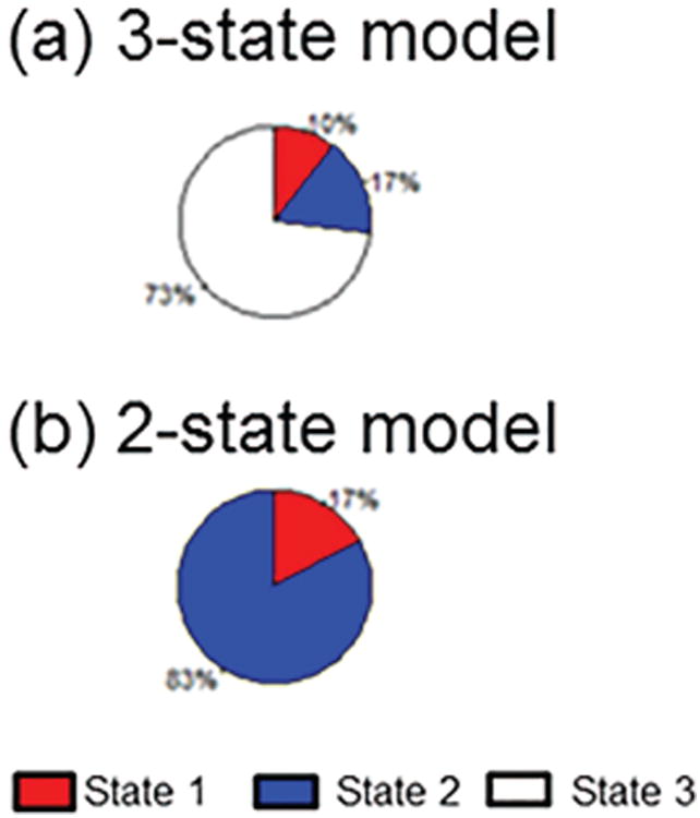
Stationary distribution of global efficiency under (a) 3-state model and (b) 2-state model in TLE patients.

Appendix G. MAP estimates of ξ

Figure G.1.

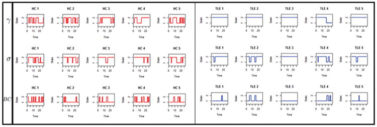
Estimated states for clustering coefficient (γ), small-world index (σ) and betweenness centrality (BC), for individual healthy controls and TLE patients, based on MAP estimates of ξ. A few representative subjects are shown. Other subjects were similar (not shown).

References

- 1.Rubinov M, Sporns O. Complex network measures of brain connectivity: Uses and interpretations. NeuroImage. 2010;52(3):1059–1069. doi: 10.1016/j.neuroimage.2009.10.003. [DOI] [PubMed] [Google Scholar]
- 2.Bullmore ET, Bassett DS. Brain graphs: Graphical models of the human brain connectome. Annual Review of Clinical Psychology. 2011;7:113–140. doi: 10.1146/annurev-clinpsy-040510-143934. [DOI] [PubMed] [Google Scholar]
- 3.Stam CJ, Reijneveld JC. Graph theoretical analysis of complex networks in the brain. Nonlinear Biomedical Physics. 2007;1(1):3. doi: 10.1186/1753-4631-1-3. [DOI] [PMC free article] [PubMed] [Google Scholar]
- 4.Ponten S, Douw L, Bartolomei F, Reijneveld J, Stam C. Indications for network regularization during absence seizures: Weighted and unweighted graph theoretical analyses. Experimental Neurology. 2009;217(1):197–204. doi: 10.1016/j.expneurol.2009.02.001. [DOI] [PubMed] [Google Scholar]
- 5.Vlooswijk M, Vaessen M, Jansen J, de Krom M, Majoie H, Hofman P, Aldenkamp A, Backes W. Loss of network efficiency associated with cognitive decline in chronic epilepsy. Neurology. 2011;77(10):938–944. doi: 10.1212/WNL.0b013e31822cfc2f. [DOI] [PubMed] [Google Scholar]
- 6.Chiang S, Haneef Z. Graph theory findings in the pathophysiology of temporal lobe epilepsy. Clinical Neurophysiology. 2014;125(7):1295–1305. doi: 10.1016/j.clinph.2014.04.004. [DOI] [PMC free article] [PubMed] [Google Scholar]
- 7.Wilke C, Worrell G, He B. Graph analysis of epileptogenic networks in human partial epilepsy. Epilepsia. 2011;52(1):84–93. doi: 10.1111/j.1528-1167.2010.02785.x. [DOI] [PMC free article] [PubMed] [Google Scholar]
- 8.Vlooswijk M, Jansen J, Majoie H, Hofman P, de Krom M, Aldenkamp A, Backes W. Functional connectivity and language impairment in cryptogenic localization-related epilepsy. Neurology. 2010;75(5):395–402. doi: 10.1212/WNL.0b013e3181ebdd3e. [DOI] [PubMed] [Google Scholar]
- 9.Micheloyannis S, Pachou E, Stam CJ, Breakspear M, Bitsios P, Vourkas M, Erimaki S, Zervakis M. Small-world networks and disturbed functional connectivity in schizophrenia. Schizophrenia Research. 2006;87(1):60–66. doi: 10.1016/j.schres.2006.06.028. [DOI] [PubMed] [Google Scholar]
- 10.Supekar K, Menon V, Rubin D, Musen M, Greicius MD. Network analysis of intrinsic functional brain connectivity in Alzheimer's disease. PLoS Computational Biology. 2008;4(6):e1000100. doi: 10.1371/journal.pcbi.1000100. [DOI] [PMC free article] [PubMed] [Google Scholar]
- 11.Chang C, Glover GH. Time–frequency dynamics of resting-state brain connectivity measured with fMRI. NeuroImage. 2010;50(1):81–98. doi: 10.1016/j.neuroimage.2009.12.011. [DOI] [PMC free article] [PubMed] [Google Scholar]
- 12.Honey C, Sporns O, Cammoun L, Gigandet X, Thiran JP, Meuli R, Hagmann P. Predicting human resting-state functional connectivity from structural connectivity. Proceedings of the National Academy of Sciences. 2009;106(6):2035–2040. doi: 10.1073/pnas.0811168106. [DOI] [PMC free article] [PubMed] [Google Scholar]
- 13.Ma S, Calhoun VD, Phlypo R, Adalı T. Dynamic changes of spatial functional network connectivity in healthy individuals and schizophrenia patients using independent vector analysis. NeuroImage. 2014;90:196–206. doi: 10.1016/j.neuroimage.2013.12.063. [DOI] [PMC free article] [PubMed] [Google Scholar]
- 14.Deco G, Jirsa VK, McIntosh AR. Emerging concepts for the dynamical organization of resting-state activity in the brain. Nature Reviews Neuroscience. 2011;12(1):43–56. doi: 10.1038/nrn2961. [DOI] [PubMed] [Google Scholar]
- 15.Fair DA, Cohen AL, Power JD, Dosenbach NU, Church JA, Miezin FM, Schlaggar BL, Petersen SE. Functional brain networks develop from a “local to distributed” organization. PLoS Comput Biol. 2009;5(5):e1000381. doi: 10.1371/journal.pcbi.1000381. [DOI] [PMC free article] [PubMed] [Google Scholar]
- 16.van Diessen E, Zweiphenning WJ, Jansen FE, Stam CJ, Braun KP, Otte WM. Brain network organization in focal epilepsy: A systematic review and meta-analysis. PloS One. 2014;9(12):e114606. doi: 10.1371/journal.pone.0114606. [DOI] [PMC free article] [PubMed] [Google Scholar]
- 17.Stern JM, Caporro M, Haneef Z, Yeh HJ, Buttinelli C, Lenartowicz A, Mumford JA, Parvizi J, Poldrack RA. Functional imaging of sleep vertex sharp transients. Clinical Neurophysiology. 2011;122(7):1382–1386. doi: 10.1016/j.clinph.2010.12.049. [DOI] [PMC free article] [PubMed] [Google Scholar]
- 18.Haneef Z, Lenartowicz A, Yeh HJ, Levin HS, Engel J, Stern JM. Functional connectivity of hippocampal networks in temporal lobe epilepsy. Epilepsia. 2014;55(1):137–145. doi: 10.1111/epi.12476. [DOI] [PMC free article] [PubMed] [Google Scholar]
- 19.Woolrich MW, Ripley BD, Brady M, Smith SM. Temporal autocorrelation in univariate linear modeling of fMRI data. NeuroImage. 2001;14(6):1370–1386. doi: 10.1006/nimg.2001.0931. [DOI] [PubMed] [Google Scholar]
- 20.Forman SD, Cohen JD, Fitzgerald M, Eddy WF, Mintun MA, Noll DC. Improved assessment of significant activation in functional magnetic resonance imaging (fMRI): Use of a cluster-size threshold. Magnetic Resonance in medicine. 1995;33(5):636–647. doi: 10.1002/mrm.1910330508. [DOI] [PubMed] [Google Scholar]
- 21.Jenkinson M, Bannister P, Brady M, Smith S. Improved optimization for the robust and accurate linear registration and motion correction of brain images. Neuroimage. 2002;17(2):825–841. doi: 10.1016/s1053-8119(02)91132-8. [DOI] [PubMed] [Google Scholar]
- 22.Smith SM. Fast robust automated brain extraction. Human Brain Mapping. 2002;17(3):143–155. doi: 10.1002/hbm.10062. [DOI] [PMC free article] [PubMed] [Google Scholar]
- 23.Fox MD, Snyder AZ, Vincent JL, Corbetta M, Van Essen DC, Raichle ME. The human brain is intrinsically organized into dynamic, anticorrelated functional networks. Proceedings of the National Academy of Sciences of the United States of America. 2005;102(27):9673–9678. doi: 10.1073/pnas.0504136102. [DOI] [PMC free article] [PubMed] [Google Scholar]
- 24.Uddin LQ, Clare Kelly A, Biswal BB, Xavier Castellanos F, Milham MP. Functional connectivity of default mode network components: Correlation, anticorrelation, and causality. Human brain mapping. 2009;30(2):625–637. doi: 10.1002/hbm.20531. [DOI] [PMC free article] [PubMed] [Google Scholar]
- 25.Power JD, Barnes KA, Snyder AZ, Schlaggar BL, Petersen SE. Spurious but systematic correlations in functional connectivity MRI networks arise from subject motion. NeuroImage. 2012;59(3):2142–2154. doi: 10.1016/j.neuroimage.2011.10.018. [DOI] [PMC free article] [PubMed] [Google Scholar]
- 26.Zhang Y, Brady M, Smith S. Segmentation of brain MR images through a hidden Markov random field model and the expectation-maximization algorithm. IEEE Transactions on Medical Imaging. 2001;20(1):45–57. doi: 10.1109/42.906424. [DOI] [PubMed] [Google Scholar]
- 27.Jenkinson M, Smith S. A global optimisation method for robust affine registration of brain images. Medical Image Analysis. 2001;5(2):143–156. doi: 10.1016/s1361-8415(01)00036-6. [DOI] [PubMed] [Google Scholar]
- 28.Greve DN, Fischl B. Accurate and robust brain image alignment using boundary-based registration. Neuroimage. 2009;48(1):63–72. doi: 10.1016/j.neuroimage.2009.06.060. [DOI] [PMC free article] [PubMed] [Google Scholar]
- 29.Andersson JL, Jenkinson M, Smith S, et al. Non-linear registration, aka Spatial normalisation FMRIB technical report TR07JA2. FMRIB Analysis Group of the University of Oxford; [Google Scholar]
- 30.Allen EA, Damaraju E, Plis SM, Erhardt EB, Eichele T, Calhoun VD. Tracking whole-brain connectivity dynamics in the resting state. Cerebral Cortex. 2012 doi: 10.1093/cercor/bhs352. bhs352. [DOI] [PMC free article] [PubMed] [Google Scholar]
- 31.Shirer W, Ryali S, Rykhlevskaia E, Menon V, Greicius M. Decoding subject-driven cognitive states with whole-brain connectivity patterns. Cerebral Cortex. 2012;22(1):158–165. doi: 10.1093/cercor/bhr099. [DOI] [PMC free article] [PubMed] [Google Scholar]
- 32.Jones DT, Vemuri P, Murphy MC, Gunter JL, Senjem ML, Machulda MM, Przybelski SA, Gregg BE, Kantarci K, Knopman DS, et al. Non-stationarity in the resting brains modular architecture. PloS One. 2012;7(6):e39731. doi: 10.1371/journal.pone.0039731. [DOI] [PMC free article] [PubMed] [Google Scholar]
- 33.Wang JH, Zuo XN, Gohel S, Milham MP, Biswal BB, He Y. Graph theoretical analysis of functional brain networks: test-retest evaluation on short-and long-term resting-state functional MRI data. PloS One. 2011;6(7):e21976. doi: 10.1371/journal.pone.0021976. [DOI] [PMC free article] [PubMed] [Google Scholar]
- 34.Lynall ME, Bassett DS, Kerwin R, McKenna PJ, Kitzbichler M, Muller U, Bullmore E. Functional connectivity and brain networks in schizophrenia. The Journal of Neuroscience. 2010;30(28):9477–9487. doi: 10.1523/JNEUROSCI.0333-10.2010. [DOI] [PMC free article] [PubMed] [Google Scholar]
- 35.Tononi G, Sporns O, Edelman GM. A measure for brain complexity: relating functional segregation and integration in the nervous system. Proceedings of the National Academy of Sciences. 1994;91(11):5033–5037. doi: 10.1073/pnas.91.11.5033. [DOI] [PMC free article] [PubMed] [Google Scholar]
- 36.Tononi G, Edelman GM, Sporns O. Complexity and coherency: integrating information in the brain. Trends in Cognitive Sciences. 1998;2(12):474–484. doi: 10.1016/s1364-6613(98)01259-5. [DOI] [PubMed] [Google Scholar]
- 37.Fristen KJ. Imaging cognitive anatomy. Trends in Cognitive Sciences. 1997;1(1):21–27. doi: 10.1016/S1364-6613(97)01001-2. [DOI] [PubMed] [Google Scholar]
- 38.van den Heuvel MP, Sporns O. Network hubs in the human brain. Trends in cognitive sciences. 2013;17(12):683–696. doi: 10.1016/j.tics.2013.09.012. [DOI] [PubMed] [Google Scholar]
- 39.Maslov S, Sneppen K. Specificity and stability in topology of protein networks. Science. 2002;296(5569):910–913. doi: 10.1126/science.1065103. [DOI] [PubMed] [Google Scholar]
- 40.Guha S, Li Y, Neuberg D. Bayesian hidden Markov modeling of array CGH data. Journal of the American Statistical Association. 2008;103(482):485–497. doi: 10.1198/016214507000000923. [DOI] [PMC free article] [PubMed] [Google Scholar]
- 41.Cassese A, Guindani M, Tadesse MG, Falciani F, Vannucci M, et al. A hierarchical Bayesian model for inference of copy number variants and their association to gene expression. The Annals of Applied Statistics. 2014;8(1):148–175. doi: 10.1214/13-AOAS705. [DOI] [PMC free article] [PubMed] [Google Scholar]
- 42.Rabiner LR. A tutorial on hidden markov models and selected applications in speech recognition. Proceedings of the IEEE. 1989;77(2):257–286. [Google Scholar]
- 43.Raiffa H, Schlaifer R. Applied statistical decision theory. Boston, Mass.: Harvard Business School; 1961. [Google Scholar]
- 44.Choi E, Lee C. Feature extraction based on the bhattacharyya distance. Pattern Recognition. 2003;36(8):1703–1709. [Google Scholar]
- 45.Lee C, Choi E. Bayes error evaluation of the gaussian ml classifier. IEEE Transactions on Geoscience and Remote Sensing. 2000;38(3):1471–1475. [Google Scholar]
- 46.Zucchini W, MacDonald IL. Hidden Markov models for time series: an introduction using R. CRC Press; 2009. [Google Scholar]
- 47.Sporns O, Zwi JD. The small world of the cerebral cortex. Neuroinformatics. 2004;2(2):145–162. doi: 10.1385/NI:2:2:145. [DOI] [PubMed] [Google Scholar]
- 48.Latora V, Marchiori M. Efficient behavior of small-world networks. Physical Review Letters. 2001;87(19):198701. doi: 10.1103/PhysRevLett.87.198701. [DOI] [PubMed] [Google Scholar]
- 49.Barabási AL, et al. Scale-free networks: a decade and beyond. Science. 2009;325(5939):412. doi: 10.1126/science.1173299. [DOI] [PubMed] [Google Scholar]
- 50.Barahona M, Pecora LM. Synchronization in small-world systems. Physical Review Letters. 2002;89(5):054101. doi: 10.1103/PhysRevLett.89.054101. [DOI] [PubMed] [Google Scholar]
- 51.Bassett DS, Bullmore E. Small-world brain networks. The Neuroscientist. 2006;12(6):512–523. doi: 10.1177/1073858406293182. [DOI] [PubMed] [Google Scholar]
- 52.Döbel B, Härtig H, Engel M. Proceedings of the Tenth ACM International Conference on Embedded Software. ACM; 2012. Operating system support for redundant multithreading; pp. 83–92. [Google Scholar]
- 53.Bartolomei F, Bettus G, Stam C, Guye M. Interictal network properties in mesial temporal lobe epilepsy: A graph theoretical study from intracerebral recordings. Clinical Neurophysiology. 2013;124(12):2345–2353. doi: 10.1016/j.clinph.2013.06.003. [DOI] [PubMed] [Google Scholar]
- 54.Bernhardt BC, Chen Z, He Y, Evans AC, Bernasconi N. Graph-theoretical analysis reveals disrupted small-world organization of cortical thickness correlation networks in temporal lobe epilepsy. Cerebral Cortex. 2011;21(9):2147–2157. doi: 10.1093/cercor/bhq291. [DOI] [PubMed] [Google Scholar]
- 55.Bonilha L, Nesland T, Martz GU, Joseph JE, Spampinato MV, Edwards JC, Tabesh A. Medial temporal lobe epilepsy is associated with neuronal fibre loss and paradoxical increase in structural connectivity of limbic structures. Journal of Neurology, Neurosurgery & Psychiatry. 2012 doi: 10.1136/jnnp-2012-302476. jnnp–2012. [DOI] [PMC free article] [PubMed] [Google Scholar]
- 56.Horstmann MT, Bialonski S, Noennig N, Mai H, Prusseit J, Wellmer J, Hinrichs H, Lehnertz K. State dependent properties of epileptic brain networks: Comparative graph–theoretical analyses of simultaneously recorded EEG and MEG. Clinical Neurophysiology. 2010;121(2):172–185. doi: 10.1016/j.clinph.2009.10.013. [DOI] [PubMed] [Google Scholar]
- 57.Vaessen MJ, Jansen JF, Vlooswijk MC, Hofman PA, Majoie HM, Aldenkamp AP, Backes WH. White matter network abnormalities are associated with cognitive decline in chronic epilepsy. Cerebral Cortex. 2011;22(9):2139–2147. doi: 10.1093/cercor/bhr298. [DOI] [PubMed] [Google Scholar]
- 58.Liao W, Zhang Z, Pan Z, Mantini D, Ding J, Duan X, Luo C, Lu G, Chen H. Altered functional connectivity and small-world in mesial temporal lobe epilepsy. PloS One. 2010;5(1):e8525. doi: 10.1371/journal.pone.0008525. [DOI] [PMC free article] [PubMed] [Google Scholar]
- 59.Bullmore E, Sporns O. Complex brain networks: graph theoretical analysis of structural and functional systems. Nature Reviews Neuroscience. 2009;10(3):186–198. doi: 10.1038/nrn2575. [DOI] [PubMed] [Google Scholar]
- 60.Stam C, De Haan W, Daffertshofer A, Jones B, Manshanden I, Van Walsum AVC, Montez T, Verbunt J, De Munck J, Van Dijk B, et al. Graph theoretical analysis of magnetoencephalographic functional connectivity in Alzheimer's disease. Brain. 2009;132(1):213–224. doi: 10.1093/brain/awn262. [DOI] [PubMed] [Google Scholar]
- 61.Chiang S, Levin HS, Haneef Z. Computer-automated focus lateralization of temporal lobe epilepsy using fMRI. Journal of Magnetic Resonance Imaging. 2014;41(6):1689–1694. doi: 10.1002/jmri.24696. [DOI] [PMC free article] [PubMed] [Google Scholar]
- 62.Zhang X, Tokoglu F, Negishi M, Arora J, Winstanley S, Spencer DD, Constable RT. Social network theory applied to resting-state fMRI connectivity data in the identification of epilepsy networks with iterative feature selection. Journal of Neuroscience Methods. 2011;199(1):129–139. doi: 10.1016/j.jneumeth.2011.04.020. [DOI] [PMC free article] [PubMed] [Google Scholar]
- 63.Eavani H, Satterthwaite TD, Gur RE, Gur RC, Davatzikos C. Information Processing in Medical Imaging. Springer; 2013. Unsupervised learning of functional network dynamics in resting state fMRI; pp. 426–437. [DOI] [PMC free article] [PubMed] [Google Scholar]
- 64.Cui S, Guha S, Ferreira MA, Tegge AN, et al. hmmSeq: A hidden Markov model for detecting differentially expressed genes from RNA-seq data. The Annals of Applied Statistics. 2015;9(2):901–925. [Google Scholar]
- 65.Fox E, Sudderth E, Jordan M, Willsky A. A sticky HDP-HMM with application to speaker diarization. Annals of Applied Statistics. 2011;5(2A):1020–1056. [Google Scholar]
- 66.Airoldi E, Costa T, Bassetti F, Leisen F, Guindani M. Generalized species sampling priors with latent beta reinforcements. Journal of the American Statistical Association. 2014;109(508):1466–1480. doi: 10.1080/01621459.2014.950735. [DOI] [PMC free article] [PubMed] [Google Scholar]
- 67.Friedman J, Hastie T, Tibshirani R. Sparse inverse covariance estimation with the graphical lasso. Biostatistics. 2008;9(3):432–441. doi: 10.1093/biostatistics/kxm045. [DOI] [PMC free article] [PubMed] [Google Scholar]
- 68.Tjandra T, Brooks JC, Figueiredo P, Wise R, Matthews PM, Tracey I. Quantitative assessment of the reproducibility of functional activation measured with BOLD and MR perfusion imaging: Implications for clinical trial design. Neuroimage. 2005;27(2):393–401. doi: 10.1016/j.neuroimage.2005.04.021. [DOI] [PubMed] [Google Scholar]
- 69.Kaufman L, Rousseeuw PJ. Finding groups in data: An introduction to cluster analysis. Vol. 344. John Wiley & Sons; 2009. [Google Scholar]