RapMap: a rapid, sensitive and accurate tool for mapping RNA-seq reads to transcriptomes

Abstract

Motivation: The alignment of sequencing reads to a transcriptome is a common and important step in many RNA-seq analysis tasks. When aligning RNA-seq reads directly to a transcriptome (as is common in the de novo setting or when a trusted reference annotation is available), care must be taken to report the potentially large number of multi-mapping locations per read. This can pose a substantial computational burden for existing aligners, and can considerably slow downstream analysis.

Results: We introduce a novel concept, quasi-mapping, and an efficient algorithm implementing this approach for mapping sequencing reads to a transcriptome. By attempting only to report the potential loci of origin of a sequencing read, and not the base-to-base alignment by which it derives from the reference, RapMap—our tool implementing quasi-mapping—is capable of mapping sequencing reads to a target transcriptome substantially faster than existing alignment tools. The algorithm we use to implement quasi-mapping uses several efficient data structures and takes advantage of the special structure of shared sequence prevalent in transcriptomes to rapidly provide highly-accurate mapping information. We demonstrate how quasi-mapping can be successfully applied to the problems of transcript-level quantification from RNA-seq reads and the clustering of contigs from de novo assembled transcriptomes into biologically meaningful groups.

Availability and implementation: RapMap is implemented in C ++11 and is available as open-source software, under GPL v3, at https://github.com/COMBINE-lab/RapMap.

Contact: rob.patro@cs.stonybrook.edu

Supplementary information: Supplementary data are available at Bioinformatics online.

1 Introduction

The bioinformatics community has put tremendous effort into building a wide array of different tools to solve the read-alignment problem efficiently. These tools use many different strategies to quickly find potential alignment locations for reads; for example, Bowtie (Langmead et al., 2009), Bowtie 2 (Langmead and Salzberg, 2012), BWA (Li and Durbin, 2009) and BWA-mem (Li, 2013) use variants of the FM-index, while tools like the Subread aligner (Liao et al., 2013), Maq (Li et al., 2008) and MrsFast (Hach et al., 2010) use k-mer-based indices to help align reads efficiently. Because read alignment is such a ubiquitous task, the goal of such tools is often to provide accurate results as quickly as possible. Indeed, recent alignment tools like STAR (Dobin et al., 2013) demonstrate that rapid alignment of sequenced reads is possible, and tools like HISAT (Kim et al., 2015) demonstrate that this speed can be achieved with only moderate memory usage. When reads are aligned to a collection of reference sequences that share a substantial amount of sub-sequence (near or exact repeats), a single read can have many potential alignments, and considering all such alignment can be crucial for downstream analysis (e.g. considering all alignment locations for a read within a transcriptome for the purpose of quantification, Li and Dewey (2011), or when attempting to cluster de novo assembled contigs by shared multi-mapping reads, Davidson and Oshlack, 2014). However, reporting multiple potential alignments for each read is a difficult task, and tends to substantially slow down even efficient alignment tools.

Yet, in many cases, all of the information provided by the alignments is not necessary. For example, in the transcript analysis tasks mentioned above, simply the knowledge of the transcripts and positions to which a given read maps well is sufficient to answer the questions being posed. In support of such ‘analysis-efficient’ computation, we propose a novel concept, called quasi-mapping, and an efficient algorithm implementing quasi-mapping (exposed in the software tool RapMap) to solve the problem of mapping sequenced reads to a target transcriptome. This algorithm is considerably faster than state-of-the-art aligners, and achieves its impressive speed by exploiting the structure of the transcriptome (without requiring an annotation), and eliding the computation of full-alignments (e.g. CIGAR strings). Further, our algorithm produces mappings that meet or exceed the accuracy of existing popular aligners under different metrics of accuracy. Finally, we demonstrate how the mappings produced by RapMap can be used in the downstream analysis task of transcript-level quantification from RNA-seq data, by modifying the Sailfish (Patro et al., 2014) tool to take advantage of quasi-mappings, as opposed to individual k-mer counts, for transcript quantification. We also demonstrate how quasi-mappings can be used to effectively cluster contigs from de novo assemblies. We show that the resulting clusterings are of comparable or superior accuracy to those produced by recent methods such as CORSET (Davidson and Oshlack, 2014), but that they can be computed much more quickly using quasi-mapping.

2 Methods

The quasi-mapping concept, implemented in the tool RapMap, is a new mapping technique to allow the rapid and accurate mapping of sequenced fragments (single or paired-end reads) to a target transcriptome. RapMap exploits a combination of data structures—a hash table, suffix array (SA) and efficient rank data structure. It takes into account the special structure present in transcriptomic references, as exposed by the SA, to enable ultra-fast and accurate determination of the likely loci of origin of a sequencing read. Rather than a standard alignment, quasi-mapping produces what we refer to as fragment mapping information. In particular, it provides, for each query (fragment), the reference sequences (transcripts), strand and position from which the query may have likely originated. In many cases, this mapping information is sufficient for downstream analysis. For example, tasks like transcript quantification, clustering of de novo assembled transcripts and filtering of potential target transcripts can be accomplished with this mapping information. However, this method does not compute the base-to-base alignment between the query and reference. Thus, such mappings may not be appropriate in every situation in which alignments are currently used (e.g. variant detection).

We note here that the concept of quasi-mapping shares certain motivations with the notions of lightweight-alignment (Patro et al., 2015) and pseudoalignment (Bray et al., 2016). Yet, all three concepts—and the algorithms and data structures used to implement them—are distinct and, in places, substantially different. Lightweight-alignment scores potential matches based on approximately consistent chains of super-maximal exact matches shared between the query and targets. Therefore, it typically requires some more computation than the other methods, but allows the reporting of a score with each returned mapping and a more flexible notion of matching. Pseudoalignment, as implemented in Kallisto, refers only to the process of finding compatible targets for reads by determining approximately matching paths in a colored De Bruijn graph of a pre-specified order. Among compatible targets, extra information concerning the mapping (e.g. position and orientation) can be extracted post hoc, but this requires extra processing, and the resulting mapping is no longer technically a pseudoalignment. Quasi-mapping seeks to find the best mappings (targets and positions) for each read, and does so (approximately) by finding minimal collections of dynamically sized, right-maximal, matching contexts between target and query positions. Quasi-mapping is inspired by both lightweight-alignment (Patro et al. (2015)) and pseudoalignment (Bray et al., 2016), and while each of these approaches provide some insight into the problems of alignment and mapping, they represent distinct concepts and exhibit unique characteristics in terms of speed and accuracy, as demonstrated below (We do not compare against lightweight-alignment here, as no stand-alone implementation of this approach is currently available).

2.1 An algorithm for Quasi-mapping

The algorithm we use for quasi-mapping makes use of two main data structures, the generalized SA (Manber and Myers, 1993) SA[T] of the transcriptome T, and a hash table h mapping each k-mer occurring in T to its SA interval (by default k  =  31). Additionally, we must maintain the original text T on which the SA was constructed, and the name and length of each of the original transcript sequences. T consists of a string in which all transcript sequences are joined together with a special separator character. Rather than designating a separate terminator ${\$}_i$ for each reference sequence in the transcriptome, we make use of a single separator $, and maintain an auxiliary rank data structure, which allows us to map from an arbitrary position in the concatenated text to the index of the reference transcript in which it appears. We use the rank9b algorithm and data structure of Vigna (2008) to perform the rank operation quickly.

Quasi-mapping determines the mapping locations for a query read r through repeated application of (i) determining the next hash table k-mer that starts past the current query position, (ii) computing the maximum mappable prefix (MMP) of the query beginning with this k-mer and then (iii) determining the next informative position (NIP) by performing a longest common prefix (LCP) query on two specifically chosen suffixes in the SA.

The algorithm begins by hashing the k-mers of r, from left-to-right (a symmetric procedure can be used for mapping the reverse-complement of a read), until some k-mer k_i—the k-mer starting at position i within the read—is present in h and maps to a valid SA interval. We denote this interval as $\mathrm{I}\left(k_i\right)=\left[b,e\right)$. Because of the lexicographic order of the suffixes in the SA, we immediately know that this k-mer is a prefix of all of the suffixes appearing in the given interval. However, it may be possible to extend this match to some longer substring of the read beginning with k_i. In fact, the longest substring of the read that appears in the reference and is prefixed by k_i is exactly the MMP (Dobin et al., 2013) of the suffix of the read beginning with k_i. We call this MMP_i, and note that it can be found using a slight variant of the standard SA binary search (Manber and Myers, 1993) algorithm. For speed and simplicity, we implement the ‘simple accelerant’ binary search variant of Gusfield (1997). Because we know that any substring that begins with k_i must reside in the interval [b,e), we can restrict the MMP_i search to this region of the SA, which is typically small.

After determining the length of MMP_i within the read, one could begin the search for the next mappable SA interval at the position following this MMP. However, though the current substring of the read will differ from all of the reference sequence suffixes at the base following MMP_i, the suffixes occurring at the lower and upper bounds of the SA interval corresponding to MMP_i may not differ from each other (see Fig. 1). That is, if $\mathrm{I}\left({\text{MMP}}_i\right)=\left[b\prime ,e\prime \right)$ is the SA interval corresponding to MMP_i, it is possible that $\left|\mathrm{LCP}\left(\mathrm{T}\left[\mathrm{SA}\left[b\prime \right]\right],\mathrm{T}\left[\mathrm{SA}\left[e\prime -1\right]\right])\right)\right|>\left|{\text{MMP}}_i\right|$. In this case, it is most likely that the read and the reference sequence bases following MMP_i disagree as the result of a sequencing error, not because the (long) MMP discovered between the read and reference is a spurious match. Thus, beginning the search for the next MMP at the subsequent base in the read may not be productive, as the matches for this substring of the query may not be informative—that is, such a search will likely return the same (relative) positions and set of transcripts. To avoid querying for such substrings, we define and make use of the notion of the NIP. The notion of the NIP in the algorithm we present for quasi-mapping is motivated by the ‘k-mer skipping’ approach adopted in Kallisto (Bray et al., 2016), though the manner in which this information is obtained is different (as are actual positions themselves), since the NIPs computed for quasi-mapping depend on the preceding matching context, which is of a dynamic and variable length. For a MMP_i, with $\mathrm{I}\left({\text{MMP}}_i\right)=\left[b\prime ,e\prime \right)$, we define $\mathrm{NIP}({\text{MMP}}_i)=\left|\mathrm{LCP}\left(\mathrm{T}\left[\mathrm{SA}\left[b\prime \right]\right],\mathrm{T}\left[\mathrm{SA}\left[e\prime -1\right]\right])\right)\right|+1$. Intuitively, the NIP of prefix MMP_i is designed to return the next position in the query string where a SA search is likely to yield a set of transcripts different from those contained in $\mathrm{I}\left({\text{MMP}}_i\right)$. To compute the LCP between two suffixes when searching for the NIP, we use the ‘direct min’ algorithm of Ilie et al. (2010). We found this to be the fastest approach. Additionally, it does not require the maintenance of an LCP array or other auxiliary tables aside from the standard SA.

Fig. 1.

The transcriptome (consisting of transcripts $t_1,\dots ,t_6$) is converted into a $\$$-separated string, T, on which a suffix array, SA[T], and a hash table, h, are constructed. The mapping operation begins with a k-mer (here, k = 3) mapping to an interval $\left[b,e\right)$ in SA[T]. Given this interval and the read, MMP_i and NIP(MMP_i) are calculated as described in section 2. The search for the next hashable k-mer begins k bases before NIP(MMP_i)

Given the definitions we have explained above, we can summarize the quasi-mapping procedure as follows (an illustration of the mapping procedure is provided in Fig. 1). First, a read is scanned from left to right (a symmetric procedure can be used for mapping the reverse-complement of a read) until a k-mer k_i is encountered that appears in h. A lookup in h returns the SA interval $\mathrm{I}\left(k_i\right)$ corresponding to the substring of the read consisting of this k-mer. Then, the procedure described above is used to compute MMP_i and $\ell =\mathrm{NIP}$(MMP_i). The search procedure then advances to position $i+\ell -k$ in the read, and again begins hashing the k-mers it encounters. This process of determining the MMP and NIP of each processed k-mer and advancing to the NIP in the read continues until the NIP exceeds position $l_r-k$ where $l_r$ is the length of the read r. The result of applying this procedure to a read is a set $S=\{\left(q_0,o_0,\left[b_0,e_0\right)\right),\left(q_1,o_1,\left[b_1,e_1\right)\right),\dots \}$ of query positions, MMP orientations and SA intervals, with one such triplet corresponding to each MMP.

The final set of mappings is determined by a consensus mechanism. Specifically, the algorithm reports the intersection of transcripts appearing in all hits—i.e. the set of transcripts that appear (in a consistent orientation) in every SA interval appearing in S. These transcripts, and the corresponding strand and location on each, are reported as quasi-mappings of this read. This lightweight consensus mechanism is inspired by Kallisto (Bray et al., 2016), though certain differences exist (e.g. quasi-mapping requires all hits to be orientation-consistent, and, since transcript identifiers are obtained from generalized transcriptome positions via a rank calculation, the mapping positions for each hit—and therefore, each read—are immediately available, rather than decodable as auxiliary information). These mappings are reported in a samtools-compatible format in which the relevant information (e.g. target id, position, strand, pair status) is computed from the mapping. We note that alternative consensus mechanisms, both more and less stringent, are easy to enforce given the information contained in the hits (e.g. ensuring that the hits are co-linear with respect to both the query and reference can be done by passing RapMap the -c flag, and δ-consistency (Patro et al., 2015) can also be easily enforced). However, below, we consider this simple consensus mechanism.

Intuitively, RapMap’s combination of speed and accuracy result from the manner in which it exploits the nature of exactly repeated sequence that is prevalent in transcriptomes (either as a result of alternative splicing or paralogous genes). In addition to efficient search for MMPs and NIPs, the SA allows RapMap to encode exact matches between the query and many potential transcripts efficiently (in the form of ‘hits’). This is because all reference locations for a given MMP appear in consecutive entries of the SA, and can be encoded efficiently by simply recording the SA interval corresponding to this MMP. By aggressively filtering the hits to determine the set of ‘best’ matching transcripts and positions, RapMap is able to quickly discard small matches that are unlikely to correspond to a correct mapping. Similarly, the large collection of exact matches that appear in the reported mapping are likely to appear in the alignment (were the actual alignments to be computed). In some sense, the success of the strategy adopted by RapMap further validates the claim of Liao et al. (2013) that the seed-and-vote paradigm can be considerably more efficient than the seed-and-extend paradigm, as RapMap adopts neither of these paradigms directly, but its approach is more similar to the former than the latter.

In the next section, we analyze how this algorithm for quasi-mapping, as described above, compares with other aligners in terms of speed and mapping accuracy.

3 Mapping speed and accuracy

To test the practical performance of quasi-mapping, we compared RapMap against a number of existing tools, and analyzed both the speed and accuracy of these tools on synthetic and experimental data. Benchmarking was performed against the popular aligners Bowtie 2 (Langmead and Salzberg, 2012) (v2.2.6) and STAR (Dobin et al., 2013) (v2.5.0c) and the recently introduced pseudoalignment procedure used in the quantification tool Kallisto (Bray et al., 2016) (v0.42.4). All experiments were scripted using Snakemake (Köster and Rahmann, 2012) and performed on a 64-bit linux server with 256 GB of RAM and 4 × 6-core Intel Xeon E5-4607 v2 CPUs running at 2.60 GHz. Wall-clock time was recorded using the time command.

In our testing we find that Bowtie 2 generally performs well in terms of reporting the true read origin among its set of multi-mapping locations. However, it takes considerably longer and tends to return a larger set of multi-mapping locations than the other methods. In comparison with Bowtie 2, STAR is substantially faster but somewhat less accurate. RapMap achieves accuracy comparable or superior to Bowtie 2, while simultaneously being much faster than even STAR. Kallisto is similar to (slightly slower than) RapMap in terms of single-threaded speed, and exhibits accuracy similar to that of STAR. For both RapMap and Kallisto, simply writing the output to disk tends to dominate the time required for large input files with significant multi-mapping (though we eliminate this overhead when benchmarking). This is due, in part, to the verbosity of the standard SAM format in which results are reported, and suggests that it may be worth developing a more efficient and succinct output format for mapping information.

3.1 Speed and accuracy on synthetic data

To test the accuracy of different mapping and alignment tools in a scenario where we know the true origin of each read, we generated data using the Flux Simulator (Griebel et al., 2012). This synthetic dataset was generated for the human transcriptome from an annotation taken from the ENSEMBL (Cunningham et al., 2015) database consisting of 86 090 transcripts corresponding to protein-coding genes. The dataset consists of $\sim 48$ million 76 bp, paired-end reads. The detailed parameters used for the Flux Simulator can be found in Supplementary Appendix 1.2.

When benchmarking these methods, reads were aligned directly to the transcriptome, rather than to the genome. This was done because we wish to benchmark the tools in a manner that is applicable when the reference genome may not even be known (e.g. in de novo transcriptomics). The parameters of STAR (see Supplementary Appendix 1.1) were adjusted appropriately for this purpose (e.g. to dis-allow introns). Similarly, Bowtie 2 was also used to align reads directly to the target transcriptome; the parameters for Bowtie 2 are given in Supplementary Appendix 1.1.

3.1.1 Mapping speed

We wish to measure, as directly as possible, just the time required by the mapping algorithms of the different tools. Thus, when benchmarking the runtime of different methods, we do not save the resulting alignments to disk. Further, to mitigate the effect of ‘outliers’ (a small number of reads which map to a large number of low-complexity reference positions), we bound the number of different transcripts to which a read can map to be 200.

Additionally, we have also benchmarked Kallisto, but have not included the results in Figure 2, as the software, unlike the other methods, does not allow multi-threaded execution if mappings are being reported. Thus, we ran Kallisto with a single thread, using the –pseudobam flag and redirecting output to /dev/null to avoid disk overhead. Kallisto requires 17.87 m to map the 48M simulated reads, which included <1 m of quantification time. By comparison, RapMap required 11.65 m to complete with a single thread.

Fig. 2.

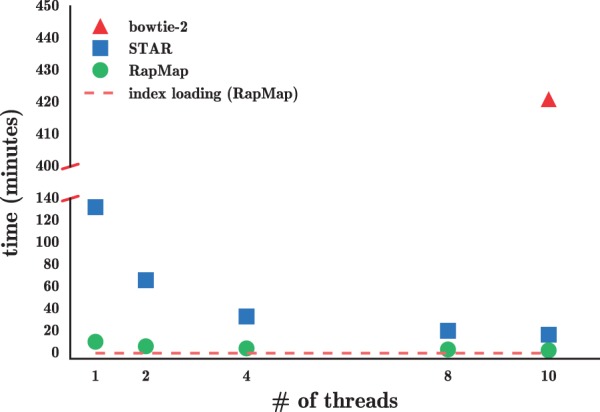
The time taken by Bowtie 2, STAR and RapMap to process the synthetic data using varying numbers of threads. RapMap processes the data substantially faster than the other tools, while providing results of comparable or better accuracy

Finally, we note Kallisto, STAR and RapMap require 2–3× the memory of Bowtie 2, but all of the methods tested here exhibit reasonable memory usage. The synthetic set of 48 million reads can be mapped to an index of the entire human transcriptome on a typical laptop with 8 GB of RAM.

As Figure 2 illustrates, RapMap outperforms both Bowtie 2 and STAR in terms of speed by a substantial margin, and finishes mapping the reads with a single thread faster than STAR and Bowtie 2 with 10 threads. We consider varying the number of threads used by RapMap and STAR to demonstrate how performance scales with the number of threads provided. On this dataset, RapMap quickly approaches peak performance after using only a few threads. We believe that this is not owing to limits on the scalability of RapMap, but rather because the process is so quick that, for a dataset of this size, simply reading the index constitutes a large (and growing) fraction of the total runtime (dotted line) as the number of threads is increased. Thus, we believe that the difference in runtime between RapMap and the other methods may be even larger for datasets consisting of a large number of reads, where the disk can reach peak efficiency and the multi-threaded input parser (we use the parser from the Jellyfish (Marçais and Kingsford, 2011) library) can provide input to RapMap quickly enough to make use of a larger number of threads. Because running Bowtie 2 with each potential number of threads on this dataset is time-consuming, we only consider Bowtie 2’s runtime using 10 threads.

3.1.2 Mapping accuracy

Because the Flux Simulator records the true origin of each read, we make use of this information as ground truth data to assess the accuracy of different methods. However, as a single read may have multiple, equally good alignments with respect to the transcriptome, care must be taken in defining accuracy-related terms appropriately. A read is said to be correctly mapped by a method (a true positive) if the set of transcripts reported by the mapper for this read contains the true transcript. A read is said to be incorrectly mapped by a method (a false positive) if it is mapped to some set of 1 or more transcripts, none of which are the true transcript of origin. Finally, a read is considered to be incorrectly un-mapped by a method (a false negative) if the method reports no mappings, but the transcript of origin is in the reference. Given these definitions, we report precision, recall, F1-Score and false discovery rate (FDR) in Table 1 using the standard definitions of these metrics. Additionally, we report the average number of ‘hits-per-read’ (hpr) returned by each of the methods. Ideally, we want a method to return the smallest set of mappings that contains the true read origin. However, under the chosen definition of a true-positive mapping, the number of reported mappings is not taken into account, and a result is considered a true positive so long as it contains the actual transcript of origin. The hpr metric allows one to assess how many extra mappings, on average, are reported by a particular method.

Table 1.

Accuracy of aligners/mappers under different metrics

Metric	Bowtie 2	Kallisto	RapMap	STAR
Reads aligned	47 579 567	44 804 857	47 613 536	44 711 604
Recall	97.41	91.60	97.49	91.35
Precision	98.31	97.72	98.48	97.02
F1-score	97.86	94.56	97.98	94.10
FDR	1.69	2.28	1.52	2.98
Hits per read	5.98	5.30	4.30	3.80

As expected, Bowtie 2— perhaps the most common method of directly mapping reads to transcriptomes— performs well in terms of precision and recall. However, we find that RapMap yields similar (in fact, slightly better) precision and recall. STAR and Kallisto obtain similar precision to Bowtie 2 and RapMap, but have lower recall. STAR and Kallisto perform similarly in general, though Kallisto achieves a lower (better) FDR than STAR. Taking the F1-score as a summary statistic, we observe that all methods perform reasonably well, and that, in general, alignment-based methods do not seem to be more accurate than mapping-based methods. We also observe that RapMap yields accurate mapping results that match or exceed those of Bowtie 2.

Additionally, we tested the impact of noisy reads (i.e. reads not generated from the indexed reference) on the accuracy of the different mappers and aligners. To create these background reads, we use a model inspired by (Gilbert et al., 2004), in which reads are sampled from nascent, un-spliced transcripts. The details of this experiment are included in Supplementary Appendix 1.3.

3.2 Speed and concordance on experimental data

We also explore the concordance of RapMap with different mapping and alignment approaches using experimental data from the study of Cho et al. (2014) (NCBI GEO accession SRR1293902). The sample consists of $\sim 26$ million 75 bp, paired-end reads sequenced on an Illumina HiSeq.

Because we do not know the true origin of each read, we have instead examined the agreement between the different tools (see Fig. 3). Intuitively, two tools agree on the mapping locations of a read if they align/map this read to the same subset of the reference transcriptome (i.e. the same set of transcripts). More formally, we define the elements of our universe, $\mathcal{U}$, to be tuples consisting of a read identifier and the set of transcripts returned by a particular tool. For example, if, for read r_i, tool A returns alignments to transcripts $\{t_1,t_2,t_3\}$ then $e_{Ai}=\left(r_i,\{t_1,t_2,t_3\}\right)\in \mathcal{U}$. Similarly, if tool B maps read r_i to transcripts $\{t_2,t_3,t_4\}$ then $e_{Bi}=\left(r_i,\{t_2,t_3,t_4\}\right)\in \mathcal{U}$. Here, tools $A$ and $B$ do not agree on the mapping of read r_i. Given a universe $\mathcal{U}$ thusly defined, we can use the normal notions of set intersection and difference to explore how different subsets of methods agree on the mapping locations of the sequenced reads. These concordance results are presented in Figure 3, which uses a bar plot to show the size of each set of potential intersections between the results of the tools we consider. In Figure 3 the dot matrix below the bar plot identifies the tools whose results are intersected to produce the corresponding bar. Tools producing mappings and alignments are denoted with black and red dots and bars, respectively. The left bar plot shows the size of the unique tuples produced by each tool (alignments/mappings that do not match with any other tool). The right bar plot shows the total number of tuples produced by each tool, and well as the concordance among all different subsets of tools.

Fig. 3.

Mapping agreement between subsets of Bowtie 2, STAR, Kallisto andRapMap.

Under this measure of agreement, RapMap and Kallisto appear to agree on the exact same transcript assignments for the largest number of reads. Further, RapMap and Kallisto have the largest pairwise agreements with the aligners (STAR and Bowtie 2)—that is, the traditional aligners exactly agree more often with these tools than with each other. It is important to note that one possible reason we see (seemingly) low agreement between Bowtie 2 and other methods is because the transcript alignment sets reported by Bowtie 2 are generally larger (i.e. contain more transcripts) than those returned by other methods, and thus fail to qualify under our notion of agreement. This occurs, partially, because RapMap and Kallisto (and to some extent STAR) do not tend to return sub-optimal multi-mapping locations. However, unlike Bowtie 1, which provided an option to return only the best ‘stratum’ of alignments, there is no way to require that Bowtie 2 return only the best multi-mapping locations for a read. We observe similar behavior for Bowtie 2 (i.e. that it returns a larger set of mapping locations) in the synthetic tests as well, where the average number of hits per read is higher than for the other methods (see Table 1). In terms of runtime, RapMap, STAR and Bowtie 2 take 3, 26 and 1020 min, respectively, to align the reads from this experiment using four threads. We also observed a similar trend in terms of the average number of hits per read here as we did in the synthetic dataset. The average number of hits per read on these data were 4.56, 4.68, 4.21 and 7.97 for RapMap, Kallisto, STAR and Bowtie 2, respectively.

4 Application of quasi-mapping for transcript quantification

While mapping cannot act as a stand-in for full alignments in all contexts, one problem where similar approaches have already proven useful is transcript abundance estimation. Recent work (Bray et al., 2016; Patro et al., 2014, 2015; Zhang and Wang, 2014) has demonstrated that full alignments are not necessary to obtain accurate quantification results. Rather, simply knowing the transcripts and positions where reads may have reasonably originated is sufficient to produce accurate estimates of transcript abundance. Thus, we have chosen to apply quasi-mapping to transcript-level quantification as an example application, and have implemented our modifications as an update to the Sailfish (Patro et al., 2014) software, which we refer to as quasi-Sailfish. These changes are present in the Sailfish software from version 0.7 forward. Here, we compare this updated method to the transcript-level quantification tools RSEM (Li et al., 2010), Tigar2 (Nariai et al., 2014) and Kallisto (Bray et al., 2016), the last of which is based on the pseudoalignment concept mentioned above.

4.1 Transcript quantification

In an RNA-seq experiment, the underlying transcriptome consists of M transcripts and their respective counts. The transcriptome can be represented as a set $\mathcal{X}=\{(t_1,\dots ,t_M),(c_1,\dots ,c_M)\}$, where t_i denotes the nucleotide sequence of transcript $i$ and $c_i$ denotes the number of copies of t_i in the sample. The length of transcript t_i is denoted by l_i. Under ideal, uniform, sampling conditions (i.e. without considering various types of experimental bias), the probability of drawing a fragment from a transcript t_i is proportional to its nucleotide fraction (Li et al., 2010) denoted by ${\eta }_i=\frac{c_i{l}_i}{{\sum }_{j=1}^M{c}_j{l}_j}$.

If we normalize the η_i for each transcript by its length l_i, we obtain a measure of the relative abundance of each transcript called the transcript fraction (Li et al., 2010), which is given by ${\tau }_i=\frac{\frac{{\eta }_i}{l_i}}{\sum _{j=1}\frac{{\eta }_i}{l_i}}$.

When performing transcript-level quantification, $\mathit{\eta }$ and $\mathit{\tau }$ are generally the quantities we are interested in inferring. Because they are directly related, knowing one allows us to directly compute the other. Below, we describe our approach to approximating the estimated number of reads originating from each transcript, from which we estimate $\mathit{\tau }$, and subsequently transcripts per million (TPM).

4.2 Quasi-mapping-based Sailfish

Using the quasi-mapping procedure provided by RapMap as a library, we have updated the Sailfish (Patro et al., 2014) software to make use of quasi-mapping, as opposed to individual k-mer counting, for transcript-level quantification. In the updated version of Sailfish, the index command builds the quasi-index over the reference transcriptome as described in Section 2. Given the index and a set of sequenced reads, the quant command quasi-maps the reads and uses the resulting mapping information to estimate transcript abundances.

To reduce the memory usage and computational requirements of the inference procedure, quasi-Sailfish reduces the mapping information to a set of equivalence classes over sequenced fragments. These equivalence classes are similar to those used in Nicolae et al. (2011), except that the position of each fragment within a transcript is not considered when defining the equivalence relation. Specifically, any fragments that map to exactly the same set of transcripts are placed into the same equivalence class. Following the notation of Patro et al. (2015), the equivalence classes are denoted as $\mathcal{C}=\{{\mathcal{C}}^1,{\mathcal{C}}^2,\dots \}$, and the count of fragments associated with equivalence class ${\mathcal{C}}^j$ is given by d^j. Associated with each equivalence class ${\mathcal{C}}^j$ is an ordered collection of transcript identifiers $t^j=\left(t_{j1},t_{j2},\dots \right)$, which is simply the collection of transcripts to which all equivalent fragments in this class map. We call $t^j$ the label of class ${\mathcal{C}}^j$.

4.2.1 Inferring transcript abundances

The equivalence classes $\mathcal{C}$ and their associated counts and labels are used to estimate the number of fragments originating from each transcript. The estimated count vector is denoted by $\mathit{\alpha }$, and α_i is the estimated number of reads originating from transcript t_i. In quasi-Sailfish, we use the variational Bayesian expectation maximization (VBEM) algorithm to infer the parameters (the estimated number of reads originating from each transcript) that maximize a variational objective. Specifically, we maximize a simplified version of the variational objective of Nariai et al. (2013).

The VBEM update rule can be written as a simple iterative update in terms of the equivalence classes, their counts and the prior (α₀). The iterative update rule for the VBEM is:

$${\alpha }_i^{u+1}={\alpha }_0+{\displaystyle \sum _{{\mathcal{C}}^j\in \mathcal{C}}{d}_j}\left(\frac{e^{{\gamma }_i^u}\frac{1}{\widehat{l_i}}}{{\displaystyle \sum _{t_k\in t^j}{e}^{{\gamma }_k^u}}\frac{1}{\widehat{l_k}}}\right),$$ (1)

where

$${\gamma }_i^u=\Psi ({\alpha }_0+{\alpha }_i^u)-\Psi ({\displaystyle \sum _k{\alpha }_0}+{\alpha }_k^u)$$ (2)

and $\Psi (·)$ is the digamma function. Here, $\widehat{l_i}$ is the effective length of transcript t_i, computed as in Li et al. (2010). To determine the final estimated counts—$\mathit{\alpha }$—Equation (1) is iterated until convergence. The estimated counts are considered to have converged when no transcript has estimated counts differing by >1% between successive iterations.

Given $\mathit{\alpha }$, we compute the TPM for transcript i as

$$TP{M}_i={10}^6\frac{\frac{{\alpha }_i}{\widehat{l_i}}}{\sum _j\frac{{\alpha }_j}{\widehat{l_j}}}.$$ (3)

Sailfish outputs, for each transcript, its name, length, effective length, TPM and the estimated number of reads originating from it.

4.3 Quantification performance comparison

We compared the accuracy of quasi-Sailfish (Sailfish v0.9.0; q-Sailfish in Table 2) to the transcript-level quantification tools RSEM (Li et al., 2010) (v1.2.22), Tigar 2 (Nariai et al., 2014) (v2.1) and Kallisto (Bray et al., 2016) (v0.42.4) using six different accuracy metrics and data from two different simulation pipelines. One of the simulated datasets was generated with the Flux Simulator (Griebel et al., 2012), and is the same dataset used in Section 3 to assess mapping accuracy and performance on synthetic data. The other dataset was generated using the RSEM simulator via the same methodology adopted by Bray et al. (2016). That is, RSEM was run on sample NA12716_7 of the Geuvadis RNA-seq data (Lappalainen et al., 2013) to learn model parameters and estimate true expression. The learned model was then used to generate the simulated dataset, which consists of 30 million 75 bp paired-end reads.

Table 2.

Performance evaluation of different tools along with quasi-enabled sailfish (q-Sailfish) with other tools on synthetic data generated by Flux simulator and RSEM simulator

Metric	Flux simulation				RSEM-sim simulation
	Kallisto	RSEM	q-Sailfish	Tigar 2	Kallisto	RSEM	q-Sailfish	Tigar 2
Proportionality corr.	0.74	0.78	0.75	0.77	0.91	0.93	0.91	0.93
Spearman corr.	0.69	0.73	0.70	0.72	0.91	0.93	0.91	0.93
TPEF	0.77	0.96	0.60	0.59	0.53	0.49	0.53	0.50
TPME	−0.24	−0.37	−0.10	−0.09	0.00	−0.01	0.00	0.00
MARD	0.36	0.29	0.31	0.26	0.29	0.25	0.29	0.23
wMARD	4.68	5.23	4.45	4.35	1.00	0.88	1.01	0.94

We measure the accuracy of each method based on the estimated versus true number of reads originating from each transcript, and consider six different metrics of accuracy: proportionality correlation (Lovell et al., 2015), Spearman correlation, the true positive error fraction (TPEF), the true positive median error (TPME), the mean absolute relative difference (MARD) and the weighted mean absolute relative difference (wMARD). Detailed definitions for the last four metrics are provided in Supplementary Appendix 1.5.

Each of these metrics captures a different notion of accuracy, and all are reported to provide a more comprehensive perspective on quantifier accuracy. The first two metrics—proportionality and Spearman correlation—provide a global notion of how well the estimated and true counts agree, but are fairly coarse measures. The TPEF assesses the fraction of transcripts where the estimate is different from the true count by more than some nominal fraction (here 10%). Unlike TPEF, the TPME metric takes into account the direction of the mis-estimate (i.e. is it an over or under-estimate of the true value?). However, both metrics are assessed only on truly expressed transcripts, and so provide no insight into the tendency of a quantifier to produce false positives.

The absolute relative difference (ARD) metric has the benefit of being defined on all transcripts as opposed to only those that are truly expressed and ranges from 0 (lowest) to 2 (highest). Because the values of this metric are tightly bounded, the aggregate metric, MARD, is not dominated by high expression transcripts. Unfortunately, it therefore has limited ability to capture the magnitude of mis-estimation. The wMARD metric attempts to account for the magnitude of mis-estimation, while still trying to ensure that the measure is not completely dominated by high expression transcripts. This is done by scaling each ARD_i value by the logarithm of the expression.

Table 2 shows the performance of all four quantifiers, under all six metrics, on both datasets. While all methods seem to perform reasonably well, some patterns emerge. RSEM seems to perform well in terms of the correlation metrics, but less well in terms of the TPEF, TPME and wMARD metrics (specifically in the Flux Simulator-generated dataset). This is likely a result of the lower mapping rate obtained on this data by RSEM’s strict Bowtie 2 parameters. Tigar 2 generally performs well under a broad range of metrics, and produces highly accurate results. However, it is by far the slowest method considered here, and requires over a day to complete on the Flux simulator data and almost 7 h to complete on the RSEM-sim data given 16 threads (and not including the time required for Bowtie 2 alignment of the reads). Finally, both quasi-Sailfish and Kallisto perform well in general under multiple different metrics, with quasi-Sailfish tending to produce somewhat more accurate estimates. Both of these methods also completed in a matter of minutes on both datasets.

One additional pattern that emerges is that the RSEM-sim data appears to present a much simpler inference problem compared with the Flux Simulator data. One reason for this may be that the RSEM-sim data are ‘clean’—yielding concordant mapping rates well over 99%, even under RSEM’s strict Bowtie 2 mapping parameters. As such, all methods tend to perform well on these data, and there is comparatively little deviation between the methods under most metrics.

For completeness, we also provide (in Supplementary Appendix 1.4) the results, under all of these metrics, where the true and predicted abundances are considered in terms of TPM rather than number of reads. We find that the results are generally similar, with the exception that TIGAR 2 performs considerably worse under the TPM measure.

5 Application of quasi-mapping for clustering de novo assemblies

Estimating gene-expression from RNA-seq reads is an especially challenging task when no reference genome is present. Typically, this problem is solved by performing de novo assembly of the RNA-seq reads, and subsequently mapping these reads to the resulting contigs to estimate expression. Owing to sequencing errors and artifacts, and genetic variation and repeats, de novo assemblers often fragment individual isoforms into separate assembled contigs. Davidson and Oshlack (2014) argue that better differential expression results can be obtained in de novo assemblies if contigs are first clustered into groups. They present a tool, CORSET, to perform this clustering, and compare their approach to existing tools such as CD-HIT (Fu et al., 2012). CD-HIT compares the sequences (contigs) directly, and clusters them by sequence similarity. CORSET, alternatively, aligns reads to contigs (allowing multi-mapping) and defines a distance between each pair of contigs based on the number of multi-mapping reads shared between them, and the changes in estimated expression inferred for these contigs under different conditions. Hierarchical agglomerative clustering is then performed on these distances to obtain a clustering of contigs.

Here, we show how RapMap can be used for the same task, by taking an approach similar to that of CORSET. First, we map the RNA-seq reads to the target contigs and simultaneously construct equivalence classes over the mapped fragments as in Section 4. We construct a weighted, undirected graph from these equivalence classes as follows. Given a set of contigs c and the equivalence classes $\mathcal{C}$, we construct $G=(V,E)$ such that $V=c$, and $E=\left\{\right\{u,v\left\}\right|\exists j:u,v\in t^j\}$. We define the weight of edge $\{u,v\}$ as $w(u,v)=\frac{R_{u,v}}{\min \left(R_u,R_v\right)}$. Here R_u is the total number of reads belonging to all equivalence classes in which contig u appears in the label. R_v is defined analogously. $R_{u,v}$ is the total sum of reads in all equivalence classes for which contigs $u$ and $v$ appear in the label. Given the undirected graph G, we use the Markov Cluster Algorithm, as implemented in MCL (Van Dongen, 2000), to cluster the graph.

To benchmark the time and accuracy of our clustering scheme compared with CD-HIT and CORSET, we used two datasets from the CORSET paper (Davidson and Oshlack, 2014). The first dataset consists of 231 million human reads in total, across two conditions, each with three replicates (as originally described by Trapnell et al., 2013). The second dataset, from yeast, was originally published by Nookaew et al. (2012) and consists 36 million reads, grown in two different conditions with three replicates each. For both of these datasets, we consider clustering the contigs of the corresponding de novo assemblies, which were generated using Trinity (Grabherr et al., 2011).

To measure accuracy, we consider the precision and recall induced by a clustering with respect to the true genes from which each contig originates. Assembled contigs were mapped to annotated transcripts using BLAT (Kent, 2002), and labeled with their gene of origin. A pair of contigs from the same cluster is regarded as true positive (tp) if they are from the same gene in the ground truth set. Similarly, a pair is a false positive (fp) if they are not from same gene but are clustered together. A pair is a false negative (fn) if they are from same gene but not predicted to be in the same cluster and all the remaining pairs are true negatives (tn). With these definitions of tp, fp, tn and fn we can define precision and recall in standard manner. As shown in Table 3, when considering both precision and recall, RapMap (quasi-mapping) enabled clustering performs substantially better than CD-HIT and similar to CORSET. RapMap enabled clustering takes 8 min and 2 min to cluster the human and yeast datasets respectively—which is substantially faster than the other tools. To generate the timing results above, CD-HIT was run with 25 threads. The time recorded for CORSET consists of both the time required to align the reads using Bowtie 2 (using 25 threads) and the time required to perform the actual clustering, which is single threaded. The time recorded for RapMap enabled clustering consists of the time required to quasi-map the reads, build the equivalence classes and construct the graph (using 25 threads), plus the time required to cluster the graph with MCL (using a single thread). Overall, on these datasets, RapMap-enabled clustering appears to provide comparable or better clusterings than existing methods, and produces these clusterings much more quickly.

Table 3.

Performance of CORSET, CD-HIT and RapMap enabled clustering (R-CL) on yeast and human data

Metric	Human			Yeast
	CORSET	CD-HIT	R-CL	CORSET	CD-HIT	R-CL
precision	0.96	0.96	0.95	0.36	0.41	0.36
recall	0.56	0.37	0.60	0.63	0.36	0.71
time (min)	957	268	8	23	5	2

6 Discussion and conclusion

In this article we have argued for the usefulness of our novel approach, quasi-mapping, for mapping RNA-seq reads. More generally, we suspect that read mapping, wherein sequencing reads are assigned to reference locations, but base-to-base alignments are not computed, is a broadly useful tool. The speed of traditional aligners like Bowtie 2 and STAR is limited by the fact that they must produce optimal alignments for each location to which a read is reported to align.

In addition to showing the speed and accuracy of quasi-mapping directly, we apply it to two problems in transcriptome analysis. First, we have updated the Sailfish software to make use of the quasi-mapping information produced by RapMap, rather than direct k-mer counts, for purposes of transcript-level abundance estimation. This update improves both the speed and accuracy of Sailfish, and also reduces the complexity of its codebase. We demonstrate, on synthetic data generated via two different simulators, that the resulting quantification estimates have accuracy comparable with state-of-the-art tools. We also demonstrate the application of RapMap to the problem of clustering de novo assembled contigs, a task that has been shown to improve expression quantification and downstream differential expression analysis (Davidson and Oshlack, 2014). RapMap can produce clusterings of comparable or superior accuracy to those of existing tools, and can do so much more quickly.

However, RapMap is a stand-alone mapping program, and need not be used only for the applications we describe here. We expect that quasi-mapping will prove a useful and rapid alternative to alignment for tasks ranging from filtering large read sets (e.g. to check for contaminants or the presence or absence of specific targets) to more mundane tasks like quality control and, perhaps, even to related tasks like metagenomic and metatranscriptomic classification and abundance estimation.

We hope that the quasi-mapping concept, and the availability of RapMap and the efficient and accurate mapping algorithms it exposes, will encourage the community to explore replacing alignment with mapping in the numerous scenarios where traditional alignment information is unnecessary for downstream analysis.

References

- Bray N.L. et al. (2016) Near-optimal probabilistic RNA-seq quantification. Nature Biotech., 34(5), 525–527. [DOI] [PubMed] [Google Scholar]
- Cho H. et al. (2014) High-resolution transcriptome analysis with long-read RNA sequencing. PLoS ONE, 9, e108095.. [DOI] [PMC free article] [PubMed] [Google Scholar]
- Cunningham F. et al. (2015) Ensembl 2015. Nucleic Acids Res., 43, D662–D669. [DOI] [PMC free article] [PubMed] [Google Scholar]
- Davidson N.M., Oshlack A. (2014) Corset: enabling differential gene expression analysis for de novo assembled transcriptomes. Genome Biol., 15, 410.. [DOI] [PMC free article] [PubMed] [Google Scholar]
- Dobin A. et al. (2013) Star: ultrafast universal RNA-seq aligner. Bioinformatics, 29, 15–21. [DOI] [PMC free article] [PubMed] [Google Scholar]
- Fu L. et al. (2012) Cd-hit: accelerated for clustering the next-generation sequencing data. Bioinformatics, 28, 3150–3152. [DOI] [PMC free article] [PubMed] [Google Scholar]
- Gilbert C. et al. (2004) Elongator interactions with nascent mrna revealed by RNA immunoprecipitation. Mol. Cell, 14, 457–464. [DOI] [PubMed] [Google Scholar]
- Grabherr M.G. et al. (2011) Full-length transcriptome assembly from rna-seq data without a reference genome. Nat. Biotechnol., 29, 644–652. [DOI] [PMC free article] [PubMed] [Google Scholar]
- Griebel T. et al. (2012) Modelling and simulating generic rna-seq experiments with the flux simulator. Nucleic Acids Res., 40, 10073–10083. [DOI] [PMC free article] [PubMed] [Google Scholar]
- Gusfield D. (1997). Algorithms on Strings, Trees, and Sequences: Computer Science and Computational Biology. Cambridge University Press, New York, NY, USA. [Google Scholar]
- Hach F. et al. (2010) mrsfast: a cache-oblivious algorithm for short-read mapping. Nat. Methods, 7, 576–577. [DOI] [PMC free article] [PubMed] [Google Scholar]
- Ilie L. et al. (2010) The longest common extension problem revisited and applications to approximate string searching. J. Discrete Algorithms, 8, 418–428. [Google Scholar]
- Kent W.J. (2002) Blat–the blast-like alignment tool. Genome Res., 12, 656–664. [DOI] [PMC free article] [PubMed] [Google Scholar]
- Kim D. et al. (2015) Hisat: a fast spliced aligner with low memory requirements. Nat. Methods, 12, 357–360. [DOI] [PMC free article] [PubMed] [Google Scholar]
- Köster J., Rahmann S. (2012) Building and documenting workflows with python-based snakemake. GCB, 26, 49–56. [Google Scholar]
- Langmead B., Salzberg S.L. (2012) Fast gapped-read alignment with Bowtie 2. Nat. Methods, 9, 357–359. [DOI] [PMC free article] [PubMed] [Google Scholar]
- Langmead B. et al. (2009) Ultrafast and memory-efficient alignment of short DNA sequences to the human genome. Genome Biol., 10, R25. [DOI] [PMC free article] [PubMed] [Google Scholar]
- Lappalainen T. et al. (2013) Transcriptome and genome sequencing uncovers functional variation in humans. Nature, 501, 506–511. [DOI] [PMC free article] [PubMed] [Google Scholar]
- Li B., Dewey C. N. (2011) RSEM: accurate transcript quantification from RNA-seq data with or without a reference genome. BMC Bioinformatics, 12, 323.. [DOI] [PMC free article] [PubMed] [Google Scholar]
- Li H., Durbin R. (2009) Fast and accurate short read alignment with burrows–wheeler transform. Bioinformatics, 25, 1754–1760. [DOI] [PMC free article] [PubMed] [Google Scholar]
- Li H. et al. (2008) Mapping short dna sequencing reads and calling variants using mapping quality scores. Genome Res., 18, 1851–1858. [DOI] [PMC free article] [PubMed] [Google Scholar]
- Li B. et al. (2010) RNA-seq gene expression estimation with read mapping uncertainty. Bioinformatics, 26, 493–500. [DOI] [PMC free article] [PubMed] [Google Scholar]
- Li H. (2013). Aligning sequence reads, clone sequences and assembly contigs with BWA-MEM.
- Liao Y. et al. (2013) The Subread aligner: fast, accurate and scalable read mapping by seed-and-vote. Nucleic Acids Res., 41, e108.. [DOI] [PMC free article] [PubMed] [Google Scholar]
- Lovell D. et al. (2015) Proportionality: a valid alternative to correlation for relative data. PLoS Comput. Biol., 11, e1004075.. [DOI] [PMC free article] [PubMed] [Google Scholar]
- Manber U., Myers G. (1993) Suffix arrays: a new method for on-line string searches. SIAM J. Comput., 22, 935–948. [Google Scholar]
- Marçais G., Kingsford C. (2011) A fast, lock-free approach for efficient parallel counting of occurrences of k-mers. Bioinformatics, 27, 764–770. [DOI] [PMC free article] [PubMed] [Google Scholar]
- Nariai N. et al. (2013) Tigar: transcript isoform abundance estimation method with gapped alignment of RNA-Seq data by variational Bayesian inference. Bioinformatics, 29, 2292–2299. [DOI] [PubMed] [Google Scholar]
- Nariai N. et al. (2014) Tigar2: sensitive and accurate estimation of transcript isoform expression with longer RNA-Seq reads. BMC Genomics, 15, S5.. [DOI] [PMC free article] [PubMed] [Google Scholar]
- Nicolae M. et al. (2011) Estimation of alternative splicing isoform frequencies from rna-seq data. Algorithms Mol. Biol., 6, 9. [DOI] [PMC free article] [PubMed] [Google Scholar]
- Nookaew I. et al. (2012) A comprehensive comparison of RNA-Seq-based transcriptome analysis from reads to differential gene expression and cross-comparison with microarrays: a case study in saccharomyces cerevisiae. Nucleic Acids Res., 40, 10084–10097. [DOI] [PMC free article] [PubMed] [Google Scholar]
- Patro R. et al. (2014) Sailfish enables alignment-free isoform quantification from RNA-Seq reads using lightweight algorithms. Nat. Biotechnol., 32, 462–464. [DOI] [PMC free article] [PubMed] [Google Scholar]
- Patro R. et al. (2015) Salmon: accurate, versatile and ultrafast quantification from RNA-Seq data using lightweight-alignment. bioRxiv, 9, 021592. [Google Scholar]
- Trapnell C. et al. (2013) Differential analysis of gene regulation at transcript resolution with RNA-Seq. Nat. Biotechnol., 31, 46–53. [DOI] [PMC free article] [PubMed] [Google Scholar]
- Van Dongen S. (2000) A cluster algorithm for graphs. Rep. Inf. Syst., 10, 1–40. [Google Scholar]
- Vigna S. (2008) Broadword implementation of rank/select queries In: Experimental Algorithms. Springer, Berlin Heidelberg, pp. 154–168. [Google Scholar]
- Zhang Z., Wang W. (2014) RNA-skim: a rapid method for RNA-Seq quantification at transcript level. Bioinformatics, 30, i283–i292. [DOI] [PMC free article] [PubMed] [Google Scholar]
Associated Data
This section collects any data citations, data availability statements, or supplementary materials included in this article.