Heart rate variability estimation in photoplethysmography signals using Bayesian learning approach

Abstract

Heart rate variability (HRV) has become a marker for various health and disease conditions. Photoplethysmography (PPG) sensors integrated in wearable devices such as smart watches and phones are widely used to measure heart activities. HRV requires accurate estimation of time interval between consecutive peaks in the PPG signal. However, PPG signal is very sensitive to motion artefact which may lead to poor HRV estimation if false peaks are detected. In this Letter, the authors propose a probabilistic approach based on Bayesian learning to better estimate HRV from PPG signal recorded by wearable devices and enhance the performance of the automatic multi scale-based peak detection (AMPD) algorithm used for peak detection. The authors’ experiments show that their approach enhances the performance of the AMPD algorithm in terms of number of HRV related metrics such as sensitivity, positive predictive value, and average temporal resolution.

1. Introduction

The heart rate variability (HRV) is a measure of variation in time duration between consecutive heart beats. HRV has used widely as an indicator for stress, health, and various disease conditions [1, 2]. This Letter presents a probabilistic approach for estimating HRV from photoplethysmography (PPG) signal recorded by wearable devices.

PPG sensors integrated in wearable devices such as smart watches and phones are widely used nowadays to provide a convenient way to measure heart activities. Average heart rate can be measured by many commercial wearable gadgets. However, motion artefact still presents a challenging problem in estimating the heart rate variability in PPG signals collected by wearable devices [3–7]. This problem motivates researchers to propose algorithms that enhance the accuracy of HRV measured by those wearable PPG sensors, and enable reliable assessment of the health conditions and provide correct diagnoses.

In a PPG signal, the location of a peak represents the instant of time at which a heartbeat occurs. Thus, the computation of HRV requires accurate identification of the location of peaks in the PPG signal, which consequently leads to precise computation of time intervals between consecutive heartbeats. Many relevant features can be derived from the HRV measurements such as the number of interval differences of successive NN intervals greater than 50ms (pNN50), and the square root of the mean squared differences of successive NN intervals (RMSSD). Researchers have shown that these features can imply valuable information about various health conditions [8]. These features, however, are sensitive to any small error in identifying the correct location of peaks. Hence, accurate peak detection in the PPG signal collected by a portable device is crucial.

The nature of a PPG signal makes HRV measurements a challenging problem, especially when using a portable PPG sensor. As shown in Fig. 1, the first wave in the PPG waveform is called systolic peak and the second one is called diastolic peak. Aortic notch or dicrotic notch is a small downward deflection in the arterial pulse that separates systolic and diastolic phase. The first peak (systolic) represents the instant of time corresponding to a heartbeat, also known as R-peak. A small motion artefact can result in the diastolic peak having a higher amplitude than the systolic peak (e.g. Fig. 8), which may lead to erroneous HRV estimation if the diastolic peak is detected as the instant of heartbeat.

Fig. 1.

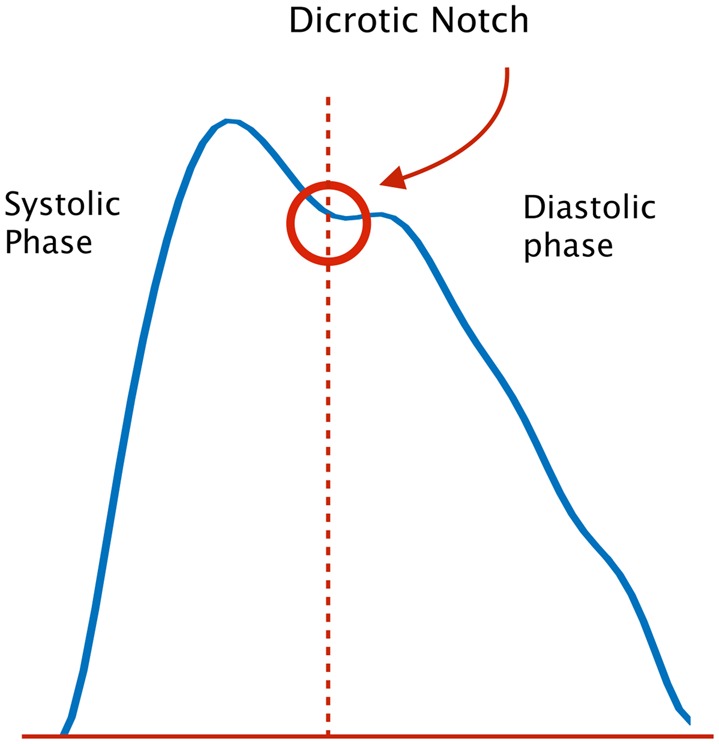
Typical PPG waveform

Fig. 8.

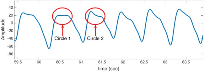
Sample of PPG signal: corrupted with some artefacts

In this Letter, we present an adaptive real-time probabilistic approach that employs Bayesian learning to estimate HRV from PPG signal recorded by wearable devices. In particular, our approach uses an algorithm called automatic multi scale-based peak detection (AMPD) [9] along with a probabilistic method to enhance its performance and provide a better HRV estimation. The proposed approach provides a soft decision on every sample in the PPG signal. We adopt a probabilistic approach that allows us to compute the probability of having a peak at every sample, and make a decision whether a peak exists in that sample by comparing the computed probability with a configured threshold. Our experiments show that the proposed algorithm enhances the AMPD algorithm with respect to a number of HRV related performance metrics such as sensitivity, positive predictive value, and average temporal resolution (ATR).

2. AMPD algorithm background

This section explains briefly the algorithm proposed by Scholkmann et al. [9]. The algorithm is called automatic multi scale-based peak detection (AMPD), and aims to detect signal peaks by analysing the local maxima scalogram (LMS) of periodic or quasi-periodic signals.

Let X = [x₁, x₂, …, x_N] be a uniformly sampled signal containing the components of a PPG signal. The AMPD algorithm calculates the LMS uses a moving window approach, whereby the window length w_k is varied (w_k = 2k|_k=1,2,…,L), where k is defined as a scale in which the PPG signal is analysed (analysis resolution). A scale could be mapped to a frequency for convenience. L represents the number of scales in the scalogram and should be defined to cover the range of frequencies that are useful for the PPG signal analysis (typically, L = 2f_s, is sufficient to include HR as low as 30 bpm, where f_s is the sampling frequency). In other words, the moving window w_k is varied at every scale k to cover different resolutions of the PPG signal. Then, a comparison criterion is performed at every scale k on the PPG signal for i = k + 2, …, N − k + 1 to search for local maxima as follows:

$$m_{k,i}=\left\{\begin{array}{cc}1& x_{i-1}>x_{i-k-1}\mathrm{and}{x}_{i-1}>x_{i+k-1}\\ 0& \mathrm{otherwise}\end{array}\right.$$ (1)

This operation results in a matrix M, where

$$\mathit{M}=\left(\begin{array}{cccc}{m}_{1,1}& m_{1,2}& \cdots & m_{1,N}\\ m_{2,1}& m_{2,2}& \cdots & m_{2,N}\\ ⋮& ⋮& \ddots & ⋮\\ m_{L,1}& m_{L,2}& \cdots & m_{L,N}\end{array}\right)=(m_{k,i})$$ (2)

where the kth row contains the value for the window length w_k. The ones in matrix M represent locations of local maxima (or the indices where potential PPG R-peaks exist) at every scale k. A PPG sample is decided to be a peak when there exists 1's for every scale k at a specific instance of time (a column in the matrix M).

3. Algorithm description

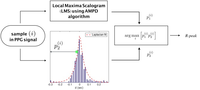
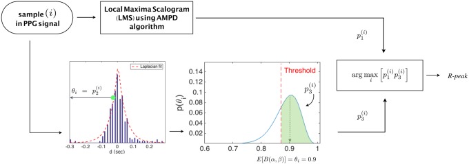
The proposed algorithm consists of two sections. Section 3.1 uses a slight modification to the output of the AMPD algorithm explained in Section 2 and exploits a model that has been built using a previous historical knowledge about R-peaks, while Section 3.2 further enhances the performance of AMPD using a probabilistic approach based on Bayesian learning. Details of the two sections are presented in the following subsections and demonstrated in Figs. 2 and 3.

Fig. 2.

Description of the algorithm design of Section 3.1

Fig. 3.

Description of the algorithm design of Section 3.2

Definition of used notations: Let us start by denoting t_j as the instant of time at which the jth R-peak occurred. We can also define the process r as the inter-arrival time between two consecutive peaks (also known as RR-intervals), namely

$$r_j=t_{j+1}-t_j$$ (3)

Another way to represent PPG peaks is by considering a process d given by the difference between consecutive RR-intervals, i.e.

$$d_j=r_{j+1}-r_j$$ (4)

The latter definition is helpful for estimating the occurrence of a next peak as will be seen next.

3.1. AMPD output modification and prior probabilistic knowledge

The AMPD algorithm works well even when a white noise is presented in a signal. Applying the algorithm to a PPG signal, which has a quasi-periodic nature, provides promising results. However, the AMPD performance degrades when the signal is corrupted with motion artefact. This is because the probabilistic characteristics of such artefact differ from the white noise.

In the AMPD algorithm, a sample is decided to be a peak if there exist ones for every scale k (i.e. all the elements in column i = 1). We modify this condition by computing p₁ of sample i as a ratio of the number of ones in column i in the matrix M to the total number of rows L, i.e.

$$p_1^{(i)}=\frac{{\sum }_{k=1}^L{m}_{k,i}}{L}$$ (5)

An enhancement could be achieved by calculating the probability of having a peak at sample i by incorporating historical previous knowledge about R-peaks. In [10], the authors show that the Laplacian model exhibits the best fit for analysing the d process. Based on their results, the probability p₂ of sample i to be a peak using Laplacian distribution is given by

$$p_2^{(i)}=\frac{1}{2b}\exp \left(-\frac{|d_i-\mu |}{b}\right)$$ (6)

Since the decision is not yet made whether sample i is a peak, d_i definition in (6) slightly differs from the general one in (4). It is defined here as d_i = r_i − r_last, where r_i represents the difference between sample i and the last detected peak, while r_last represents the last recorded RR-interval from the last cycle. μ in (6) is defined as the median. From the observed historical data of PPG signals, it is reasonable to assume that μ equals to zero. b in (6) is a scalar parameter calculated as

$$b=\frac{1}{K}\sum _{j=1}^K|d_j-\mu |,$$ (7)

where K is the number of records of the process d. To that end, one can build the decision criterion by considering the two parameters p₁ and p₂, based on the maximum probability of all samples that fall within the range of interest, i.e.

$$\mathrm{Peak}=\underset{i}{\arg max}[p_1^{(i)}{p}_2^{(i)}]$$ (8)

However, we can enhance the accuracy of a peak detection by accounting for the variation of the heart rate. To consider such cases, the constructed model should be dynamic and updated on the fly. For that reason, a Bayesian inference is proposed in the following subsection.

3.2. Probabilistic analysis and Bayesian inference formulation of the problem

Let us start by assuming that the probability of having a peak at sample i is θ_i. θ_i can be initially calculated using (6) $(\mathrm{i}.\mathrm{e}.{\theta }_i=p_2^{(i)})$. However, having a decision merely using θ_i may not be the best thing to do, given that we can learn from the incoming data. Thus, we can formulate the problem using Bayesian inference as follows

$$\begin{array}{rl}\mathrm{posterio}{\mathrm{r}}_{(i)}& =P({\theta }_i|\mathrm{AMP}{\mathrm{D}}_{\mathrm{output}(i)})\\ & =P(\mathrm{AMP}{\mathrm{D}}_{\mathrm{output}(i)}|{\theta }_i)\cdot P({\theta }_i{)}_{\mathrm{prior}}\end{array}$$ (9)

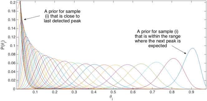
Considering the term P(θ_i)_prior in (9), it is the prior probability distribution of θ_i. We aim at finding a distribution to model P(θ_i)_prior that initially considers the probability computed in (6) as the expected value for this distribution and can be easily updated during the learning process. We used the Beta function to achieve this goal. To see why the Beta function is good to model P(θ_i), one can observe that such model results in a positively skewed probability distribution (skewed to the left) when θ_i is low (which is the case for a sample i that is close to the last detected peak), while it is negatively skewed probability distribution (skewed to the right) when θ_i is high (which is the case when sample i is close to next expected peak). Samples that are in the middle of consecutive expected peaks result in a probability distribution for θ_i that is close to the uniform distribution. Such Beta function behaviour is illustrated in Fig. 4. We observe that such statistical behaviour of the Beta distribution can be used to model P(θ_i)_prior very well. Hence, we can consider

$$P({\theta }_i{)}_{\mathrm{prior}}=\frac{\mathrm{\Gamma }(\alpha +\beta )}{\mathrm{\Gamma }(\alpha )\mathrm{\Gamma }(\beta )}{\theta }_i^{\alpha -1}(1-{\theta }_i{)}^{\beta -1}$$ (10)

where Γ is the Gamma function, and can be obtained in a tabular form corresponding to the Gamma probability distribution. Note that (Γ(α + β)/Γ(α)Γ(β)) is a normalised constant to ensure that the total probability integrates to 1. α and β are called hyper-parameters that control the shape of the distribution. We need to set those parameters such that they properly characterise a prior probability distribution for every sample i. We know that

$$E[{\theta }_{i-\mathrm{prior}}]=\alpha {/}_{\alpha +\beta },$$ (11)

when ${\theta }_{i-\mathrm{prior}}$ follows the Beta probability distribution. We initially set this expectation value to be $E[{\theta }_{i-\mathrm{prior}}]=p_2^{(i)}$. Further, we assume that (α + β) is constant, where the constant can be configured according to the implementation design. By plugging the values of $p_2^{(i)}$ and the constant (α + β) into (11), we get the desired parameters α and β that characterise the Beta distribution for a specific sample i. To summarise the discussion above, the $P({\theta }_i{)}_{\mathrm{prior}}\sim B(\alpha ,\beta )$ with an expectation value of ${\theta }_{i-\mathrm{prior}}$ equals to $p_2^{(i)}$.

Fig. 4.

Modelling for the prior probability distribution (P(θ_i)_prior) as Beta function

Going back to (9), let us consider the likelihood P(AMPD_output(i)|θ_i), where AMPD_output(i) is considered here as a binary variable representing outputs from the AMPD algorithm. In other words, AMPD_output(i) is 1 when $p_1^{(i)}$ in (5) equals to 1 and zero otherwise. Since we assume independent θ_i for every sample i (i.e. θ_i's are iid), we can think of the binary output of the AMPD algorithm at each sample i as an outcome of a Bernoulli experiment, wherein each sample i has its own θ_i. Thus, we can write

$$P(\mathrm{AMP}{\mathrm{D}}_{\mathrm{output}(i)}|{\theta }_i)={\theta }_i^n(1-{\theta }_i{)}^{1-n},\mathrm{for}n\in \{0,1\}$$ (12)

Substituting (10) and (12) into (9), we get the posterior probability distribution of θ_i as a new Beta distribution B(α′, β′), i.e.

$$\mathrm{posterio}{\mathrm{r}}_{(i)}=B({\alpha }^{\mathrm{\prime }},{\beta }^{\mathrm{\prime }})={\theta }_i^{n+\alpha -1}(1-{\theta }_i{)}^{\beta -n}$$ (13)

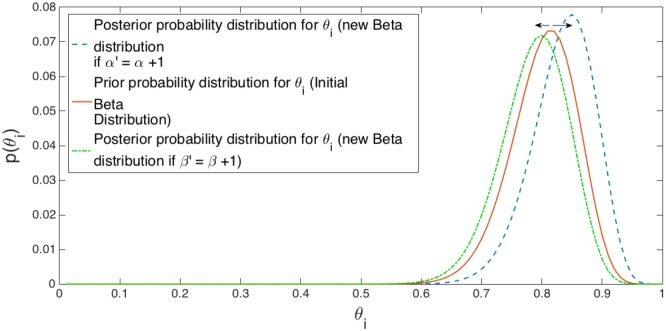
In other words, if the binary output of the AMPD algorithm at sample i equals to n = 1, then α′ = α + 1 and β′ = β, while if n = 0, then α′ = α and β′ = β + 1. It turns out that this is a simple and compact way to update the parameters of posterior_(i) at every cycle.

3.3. Learning procedure

We define a cycle as the time interval between two peaks. During that cycle, the task is to search for the next peak. In the very first cycle of the PPG sampled data, prior probability distribution for θ_i are initiated for every sample falls within the range of interest exploiting information acquired from (6). In the next cycle, the posterior probability distribution for θ_i (posterior_(i)) is computed by updating the Beta function with +1 for α or β depending on the AMPD_output(i) for that specific sample. Practically, having α′ = α + 1 results in shifting the Beta function curve to the right (increases the confidence for that sample being a peak), while having β′ = β + 1 results in shifting the Beta function curve to the left (decreases the confidence for that sample being a peak). Since this procedure is repeated for every cycle, those samples corresponding to the most probable peak locations will have a higher expected value as the distribution of their posteriors will be skewed to the right. Demonstration of this learning procedure is depicted in Fig. 5.

Fig. 5.

Explanation of the learning procedure

3.4. R-peak decision criterion

The decision of a new peak is made by considering two terms. First, the ratio $p_1^{(i)}$ acquired from the AMPD algorithm in (5). Second, the confidence value $p_3^{(i)}$ of the corresponding posterior of sample i, where $p_3^{(i)}$ is calculated as

$$p_3^{(i)}={\int }_{\mathrm{threshold}}^1\mathrm{posterio}{\mathrm{r}}_{(i)}\mathrm{d}{\theta }_i={\int }_{\mathrm{threshold}}^1\mathrm{Beta}({\alpha }^{\mathrm{\prime }},{\beta }^{\mathrm{\prime }})\mathrm{d}{\theta }_i,$$ (14)

where threshold can be configured empirically. $p_3^{(i)}$ value represents the confidence that sample i is R-peak. Note that posterior_(i) follows Beta function with a pdf that sums to one. The proposed algorithm makes a decision on R-peak by applying (15) below for all considered samples within the range of interest as follows:

$$\mathrm{Peak}=\underset{i}{\arg max}[p_1^{(i)}{p}_3^{(i)}]$$ (15)

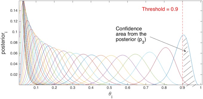
Fig. 6 illustrates the approach of calculating the value p₃ of sample i.

Fig. 6.

Posterior probability distribution of θ_i for sample i. Every graph in the figure represents posterior_(i) for sample i

We note that by incorporating information from the AMPD algorithm in Section 3.1, we are adding an independent source of information as input to the decision criterion. Moreover, the output from AMPD helps the proposed algorithm to avoid error propagation, which may happen since the decision on the next peak relies on the previously detected peak.

4. Evaluation

For the purpose of evaluating the proposed approach, an ECG signal was recorded using Zephyr BioHarness3 chest strap with sampling rate 250 Hz, from which we computed the instants of time at which we have heartbeats. The ECG results are used as a ground-truth to PPG signal algorithms under comparisons. The PPG signals were collected from an Empatica PPG sensor with a sampling rate 64 Hz.

4.1. Experimental setup and performance metrics

The recorded PPG data were processed and analysed using MATLAB simulation environment, wherein the authors of this Letter were the subjects of the experiments. We evaluated the performance in two cases. In the first case, we considered 5 min recording of artefact free PPG signal. Fig. 7 shows a sample of the PPG signal used in this experiment. To simulate the artefact in PPG signals, we considered a spike signal that follows Poisson arrivals with mean 0.25 arrival/seconds and signal amplitudes that vary with different signal-to-noise ratios (SNRs). In the second case, we considered 8 min PPG signal recording, wherein the subjects were performing different activities including: resting, walking and slow hand movement in vertical, horizontal and circular directions. This kind of physical motion results in some artefact in the PPG signal and a baseline wander.

Fig. 7.

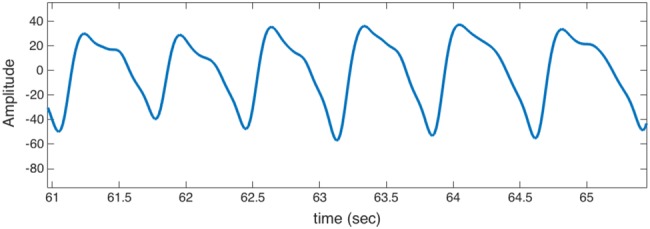
Sample of PPG signal: artefact-free

We compared our proposed algorithm against the AMPD algorithm in terms of three performance metrics: sensitivity (Se), positive predictively (+P), and ATR. Se and +P metrics were proposed by Advancement of Medical Instrumentation (AAMI) [11]. The two metrics assess the performance in terms of two expected errors: missing peaks or detecting non-existed peaks (phantoms), respectively. The two metrics are defined as follows

$$\mathrm{Se}=\frac{\mathrm{TP}}{\mathrm{TP}+\mathrm{FN}}$$ (16)

and

$$+P=\frac{\mathrm{TP}}{\mathrm{TP}+\mathrm{FP}}$$ (17)

These metrics are evaluated within an acceptance range, where the acceptance range is defined as half the time lapses between a peak and its predecessor and successor peaks in the PPG signal. When peaks are detected within the acceptance interval, they are considered as true positives (TPs). Detection of false peaks (phantoms) are referred to false positives (FPs). Missed peaks within the acceptance interval are marked as false negatives (FNs). In this sense, sensitivity (Se) indicates the percentage of true peaks that were correctly detected by the algorithm over all peaks, while positive predictive value (+P) indicates the percentage of true peaks that were correctly detected, but are not phantoms. By temporal resolution, we refer to the time accuracy where the detection of a peak using the proposed approach is compared to the ground truth peak, which is acquired from electrocardiography signal. In other words, the difference between the instant in which a peak is detected using the proposed approach (T1) and the ground truth value (T2) is computed. Taking into consideration that the PPG signal contains numerous peaks, the ATR is computed as shown in the following equation

$$\mathrm{ATR}=\frac{{\sum }_{j=1}^N|T{1}_{(j)}-T{2}_{(j)}|}{N},$$ (18)

where N is the total number of peaks in the signals.

4.2. Results and discussion

The results of the first case are shown in Figs. 9–11, while the results of the second case are shown in Table 1.

Fig. 9.

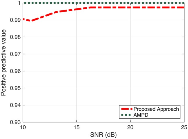
Performance evaluation: positive predictive value

Fig. 11.

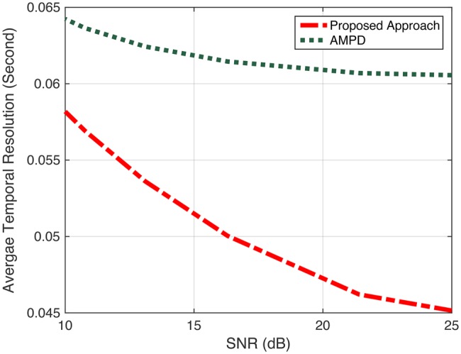
Performance evaluation: ATR

Table 1.

ATR: performance evaluation for case 2

Approach	ATR
our proposed approach	6.8 ms
AMPD	45.2 ms

PPG signal is usually exposed to different types of noise and artefacts. Fig. 8 shows a typical PPG signal where noise exists at part of the signal. Circle 2 represents a part of the signal where only one peak exists within a cycle. Such peak can be easily detected by several algorithms. On the other hand, Circle 1 shows a situation where the peak is hard to be detected. Our approach overcomes this problem by an applying Bayesian-based algorithm that utilises prior knowledge about the instant of the occurrence for several previous peaks.

In the first case, the results show a comparable performance between AMPD and our proposed algorithm in term of positive predictive value +P (Fig. 9). However, our proposed algorithm outperforms AMPD in terms of Se and ATR as shown in Figs. 10 and 11, respectively. We can observe from Fig. 10 that as SNR value decreases, the difference in Se (which is related to the number of missed peaks) increases between the two approaches. Having a high conservative algorithm when making a decision on a peak, such as AMPD, results in selecting only peaks with high confidence. Meaning that AMPD decides a sample i is a peak when this detected peak represents a global maximum for all scales. For this reason, the AMPD algorithm misses some ‘true peaks’. Therefore, AMPD has high +P, but relatively lower Se. Depending on the application at hand, +P metric may be very important, and in that case, a conservative approach for detecting peaks such as AMPD may be desirable. In any case, our approach provides a very comparable result for the case of +P, but significantly enhances the performance of Se, yielding to superior overall performance. In Fig. 11, the ATR values of AMPD increase as SNR level decreases. The proposed approach shows better performance for different SNR levels. It is observed that the difference between ATR values is decreasing as more noise is introduced to the signal.

Fig. 10.

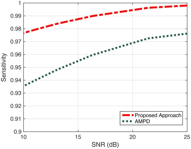
Performance evaluation: sensitivity

The results of the second case are shown in Table 1. The ATR difference between the two approaches is around 38 ms, while the Se and +P values are similar. Achieving better accuracy in temporal resolution is important as this error represents the standard deviation in heart rate that directly reflects the HRV. In [12], the authors present a quantitative systematic review of normal values for short-term heart rate variability in healthy adults. The authors showed in a tabular form a summary data including the overall range in values for each of the HRV measures. One of the important HRV measures is the standard deviation of the RR intervals (SDNN). It is known that SDNN is directly affected by the number of missed peaks (which represents the Se), phantoms (which represents +P) and the temporal accuracy of the detected peak (which is represented by ATR). It has been shown in [12] that SDNN ranges between (32 and 93) ms with mean 50 ms according to 27 studies surveyed. Table 2 shows the impact of ATR on some HRV measures including SDNN values. We can observe that, for example, SDNN computed by AMPD is outside the range of SDNN of healthy adults according to the survey in [12]. Thus, errors in peak detections may provide SDNN value that yields to erroneous diagnoses and physiological interpretation.

Table 2.

HRV measurements for case 2

HRV metric	ECG	Our approach	AMPD
SDNN	86.3	87.5	204.8
SDANN*	45.9	53.6	172.2
pNN50	18.7	24.2	63.3
RMSSD	54.6	62.7	265.9
SDNNi**	67.4	65	103.5
average HR	68.9	69	68.1

*Standard deviation of the averages of NN intervals in all 5 min segments of the entire recording

**Mean of the standard deviations of all NN intervals for all 5 min segments of the entire recording

5. Conclusion

Our proposed approach uses a Bayesian learning algorithm to estimate HRV from PPG signals. This approach enhances the performance of the AMPD algorithm and enables better HRV estimation when PPG is distorted with artefact. Our experiments show that the proposed approach has a comparable performance with the AMPD in terms of sensitivity and positive predictive values. However, it outperforms the AMPD in terms of ATR. In future work, we shall develop an accurate model for the prior probability distribution using historical observations of RR-intervals from a large dataset with different scenarios. We shall also attempt to mathematically characterise the noise that is typically associated with the PPG signals collected by wearable sensors.

6. Funding and Declaration of Interests

This work was supported by the Center of Excellence in Telecommunication Applications at King Abdulaziz City for Science and Technology, National Science, Technology and Innovation plan (NSTIP) grant numbers 34-987 and 34-988. Conflict of interest: none declared.