The second decade of 3C technologies: detailed insights into nuclear organization

Denker and de Laat describe differences and commonalities between the different 3C methods and explain how more detailed insights into the 3D genome aid in understanding transcriptional regulation in development and deregulation in disease.

Abstract

The relevance of three-dimensional (3D) genome organization for transcriptional regulation and thereby for cellular fate at large is now widely accepted. Our understanding of the fascinating architecture underlying this function is based on microscopy studies as well as the chromosome conformation capture (3C) methods, which entered the stage at the beginning of the millennium. The first decade of 3C methods rendered unprecedented insights into genome topology. Here, we provide an update of developments and discoveries made over the more recent years. As we discuss, established and newly developed experimental and computational methods enabled identification of novel, functionally important chromosome structures. Regulatory and architectural chromatin loops throughout the genome are being cataloged and compared between cell types, revealing tissue invariant and developmentally dynamic loops. Architectural proteins shaping the genome were disclosed, and their mode of action is being uncovered. We explain how more detailed insights into the 3D genome increase our understanding of transcriptional regulation in development and misregulation in disease. Finally, to help researchers in choosing the approach best tailored for their specific research question, we explain the differences and commonalities between the various 3C-derived methods.

Fifteen years have passed since the sequence of the human genome was published (Lander et al. 2001; Venter et al. 2001), and being able to read our own “instruction book” arguably demarcates one of the biggest breakthroughs in biomedical history. However, we have also learned that, in contrast to reading text in a book sentence by sentence, the genome does not just function in a sequential fashion but is folded in three-dimensional (3D) space, thereby allowing genomic elements located very remotely to contact and regulate each other, as if a word on page 10 of the instruction book would influence the meaning of a word on the very first page. In order to understand genome function, we now realize that a thorough understanding of spatial genome organization is also required.

Both conventional and superresolution microscopy as well as chromosome conformation capture (3C) technologies have provided important insights into 3D chromatin architecture. The original 3C methodology was introduced by Dekker et al. (2002): It is a biochemical procedure used to analyze in vivo contact frequencies between selected pairs of genomic sequences. In the decade following this hallmark report, the application of 3C technology and the development of high-throughput methods derived from the original 3C protocol have greatly improved our understanding of genome folding. Important principles and functional implications of genome topology have been uncovered. In 2012, we reviewed a decade of 3C technologies (de Wit and de Laat 2012). The present review aims to provide an update, summarizing the main technological advances and breakthrough findings made over the last 5 years. Together, the two reviews provide the reader with a historical and contemporary perspective on the development and application of different 3C technologies and their contribution to our understanding of structural and functional genome organization.

Basic principles of genome organization uncovered by microscopy

Although the focus of this review is on 3C technologies, it is important to realize that many basic principles of genome organization had already been uncovered by microscopy. Light and electron microscopy revealed the existence of distinct subnuclear organelles (or nuclear bodies), which, unlike cytoplasmic organelles, are not separated by membranes. Examples of nuclear bodies include the nucleolus (Pederson 2011), nuclear speckles (Spector and Lamond 2011), Cajal bodies (Cajal 1903; Nizami et al. 2010), polycomb bodies (Kerppola 2009; Pirrotta and Li 2012), and PML nuclear bodies (Lallemand-Breitenbach and de The 2010). We are only beginning to understand their functions and refer to other reviews for further information about these intriguing nuclear substructures (Mao et al. 2011). Early microscopy studies showed that active euchromatin and inactive heterochromatin occupy separate environments in the nucleus, with heterochromatin often adopting more peripheral positions (Heitz 1928). Chromosomes occupy distinct territories, with limited but appreciable intermingling (Cremer et al. 1982; Haaf and Schmid 1991; Cremer and Cremer 2001; Branco and Pombo 2006). The positioning of these territories within the nucleus is not random, but the radial alignment of chromosomes reflects their gene density, with gene-dense chromosomes such as human chromosome 19 adopting more internal nuclear positions than gene-poor chromosomes such as human chromosome 18 (Croft et al. 1999; Boyle et al. 2001). Individual genes have been observed to adopt different nuclear positions in relation to their transcriptional status, with genes being removed from the nuclear periphery or chromocenters (heterochromatic clusters of centromeres) upon activation of their expression (Brown et al. 1997, 1999; Zink et al. 2004). Live-cell imaging suggests that most endogenous mammalian genes require cell division to adopt novel nuclear locations. After mitosis in early G1, a temporary window exists during which the different parts of the genome are relatively mobile and able to find their energetically most favorable positions. Once so positioned, most genomic segments maintain their spatial location and show only local Brownian motion during the remainder of the cell cycle (Chubb et al. 2002; Walter et al. 2003; Kind et al. 2013; Bouwman and de Laat 2015). Forced recruitment of transgenes to the nuclear periphery or the chromocenters can, but does not always, influence their expression (Kumaran and Spector 2008; Reddy et al. 2008; Wijchers et al. 2015). Thus, microscopy studies revealed major principles of nuclear architecture and provided evidence for a correlation between nuclear location and transcriptional output. With recent advances in superresolution microscopy (Lakadamyali and Cosma 2015) and novel sophisticated means to follow endogenous loci with high precision in living cells (Chen et al. 2013; Saad et al. 2014; Shao et al. 2016), microscopy is expected to only become more important for nuclear organization research.

Following the introduction of the nuclear ligation assay (Cullen et al. 1993), a method already employing some of the key principles of 3C technology, the 3C methodologies introduced a very different, complementary toolbox that allowed the study of DNA folding at higher resolution and in a more systematic manner. Until recently, this could be done only at the cell population level, with 3C-based methods providing a population-averaged impression of contact frequencies between pairs of genomic sites. Now, 3C technologies are providing first insights into single-cell genome conformations. Before highlighting the latest discoveries, we first summarize early 3C work.

Early discoveries made by 3C methodologies

Originally applied to study the folding of a yeast chromosome (Dekker et al. 2002), 3C technology was quickly adapted to study long-range gene regulation and demonstrate that remote enhancers physically loop to their target genes in the β-globin locus (Tolhuis et al. 2002). Contacts between dispersed regulatory sequences and genes were found to be tissue-specific and change during development, concomitant with the activation of a different set of globin genes (Palstra et al. 2003). While enhancer–promoter interactions were found to require tissue-specific transcription factors (Drissen et al. 2004; Vakoc et al. 2005), the ubiquitously expressed CTCF protein (CCCTC-binding factor) was discovered to form loops between binding sites flanking the globin locus (Splinter et al. 2006). Regulatory enhancer–promoter loops were subsequently found at many other gene loci, as were architectural chromatin loops between CTCF sites (Handoko et al. 2011; Li et al. 2012). With initial studies primarily focusing on key developmental genes, the impression arose that enhancer loops are always established de novo exclusively in the cell type of interest. As discussed below, there is now also growing evidence for pre-established spatial conformations that appear to juxtapose regulatory sites and genes in a more tissue invariant manner. As for CTCF, this protein was mostly known for its capacity to bind to insulator elements in the genome that block the functional interplay between enhancers and promoters (for example, refer to Bell et al. 1999; Hark et al. 2000). Cohesin, a ring-shaped protein complex known to embrace and concatenate sister chromatids upon replication (for review, see Peters et al. 2008), was soon after established as a looping partner of CTCF (Parelho et al. 2008; Wendt et al. 2008; Hadjur et al. 2009).

To study genome architecture in a more systematic and genome-wide fashion, high-throughput 3C-based methods were needed. The original 3C technology, a method to study contact frequencies between selected pairs of sequences (a “one-to-one” approach), was soon followed by the development of higher-throughput variants, including “one-to-all” 4C (circularized 3C) technology (Simonis et al. 2006; Zhao et al. 2006), “many-to-many” 5C (3C carbon copy) technology (Dostie et al. 2006), and “all-to-all” Hi-C (chromosome capture followed by high-throughput sequencing) (Lieberman-Aiden et al. 2009). These methods provided independent and more detailed evidence for the existence of chromosome territories, their (limited) capacity to intermingle, and the spatial separation of active and inactive chromatin in the nucleus (Simonis et al. 2006; Lieberman-Aiden et al. 2009). Based on analysis of Hi-C data, it became evident that the genome falls into two major compartments, commonly labeled A and B (Fig. 1; Lieberman-Aiden et al. 2009). The A compartment is generally gene-rich, transcriptionally active, and accessible (as detected by DNase I sensitivity), whereas the B compartment represents a more repressed environment with fewer genes and reduced expression as well as repressive histone marks. While transvection (Pirrotta 1999) and paramutation (Chandler 2010) were well established phenomena involving regulatory communication between (paired) chromosomes in Drosophila and plants, respectively, claims based on early 3C studies for mammalian interchromosomal gene regulation were generally not followed up or were proven unlikely by genetic studies (Fuss et al. 2007). In one (artificial) instance, genetic evidence for mammalian interchromosomal gene regulation was provided: The integration of a strong enhancer on one chromosome was found to transactivate a natural target gene on another chromosome in transgenic mice. However, this occurred only in cells in which the two loci were by chance juxtaposed in their nucleus, hence resulting in variegated cellular expression (Noordermeer et al. 2011a).

Figure 1.

Hierarchical genome organization. Schematic representation of the organization of the 3D genome into A (blue) and B (red) compartments and topologically associated domains (TADs), which are composed of several sub-TADs (depicted here as spheres), which in turn harbor several chromatin loops. Panels below the respective schematics depict how these structures are perceived in Hi-C (the “checkerboard” pattern for compartments; TADs, sub-TADs, and loops as detected in the interaction matrix) and 4C (chromatin contact plot showing loops). Note, however, that domains can also be appreciated in 4C data. Arrowheads indicate loops detected in tissue 1. Bars: compartment map, 10 Mb; tissue comparison Hi-C map, 100 kb. The bottom left Hi-C panel was created using the Juicebox software (Rao et al. 2014). The top right Hi-C panel is reprinted from Krijger et al. (2016).

In summary, the advent of 3C technologies created possibilities to study DNA interactions at unprecedented detail and, later, also scale. In addition, chromatin interaction analysis by paired-end tag sequencing (ChIA-PET) provided a method to study contacts between sequences bound by a protein of interest (Fullwood et al. 2009). Early 3C studies had demonstrated that long-range communication between enhancers and genes takes place through chromatin looping and that transcription factors and CTCF, possibly with the help of cohesin, can form long-range DNA contacts between cognate binding sites. As predicted from polymer-folding models, contacts rapidly decline with increased separation on the linear chromosome template, making contact-dependent functional communication over large genomic (>>1-Mb) distances or even between chromosomes not very likely. If existing, they were predicted to lead to variegated expression.

Over the last 5 years, we have seen the maturation and broad adaptation of 3C technologies. Technical improvements combined with deeper sequencing enabled the generation of high-resolution contact maps, particularly with Hi-C and 4C. Alternative strategies were introduced, often involving a pull-down step with oligonucleotide probes to target contact analysis to specific genomic sites. 3C-based methods are now becoming a routine tool in laboratories studying topics as diverse as gene regulation, replication, chromatin, and epigenetics. In addition, they are entering the field of molecular medicine, as they have proved useful for the interpretation of disease-associated genetic variation. Here, we discuss the more recent technical advances and various applications of 3C technologies and highlight the biology unveiled by these methods. In addition, we discuss technical caveats and considerations concerning data analysis and interpretation, aiming to facilitate choosing the best approach for a given research question and identifying means for how to handle the retrieved data.

3-4-5-Hi-C and ChIA-PET: basic principles of the ‘classic’ 3C technologies

To appreciate the recent advances in 3C methods, it is important to first understand the technicalities shared between the different “classic” strategies as well as their distinguishing aspects. In all standard 3C-based protocols, chromatin is first cross-linked, most often by using formaldehyde as a fixative (see Fig. 2; Dekker et al. 2002). The cross-linked chromatin is then fragmented. Although MNase was recently introduced in a modified Hi-C procedure called Micro-C to provide nucleosome-resolution chromosome-folding maps in yeast (Hsieh et al. 2015), fragmentation so far usually involved restriction enzymes. Most commonly used restriction enzymes target either 6- or 4-base-pair (bp) recognition sequences, with the former theoretically cutting the genome every 4096 bp and the latter cutting the genome every 256 bp, which then substantially increases the resolution. Subsequent in situ ligation ensures preferential ligations between contacting and cross-linked chromatin fragments. Upon reversal of the cross-links, the so-called 3C template is obtained, which consists of linear and circular DNA concatemers carrying genomic fragments reshuffled according to their spatial proximity. This template serves as input for all 3C-based methods, which essentially differ in their strategy to detect and quantify ligation junctions.

Figure 2.

Overview of the established and newly developed 3C-derived methods. Schematics illustrate the experimental steps specific or common to the different methods. (*) DNase Hi-C has been combined with target enrichment, rendering it a “many versus all” method such as targeted chromatin capture (T2C), capture Hi-C (Chi-C), HiCap, and Capture-C. (†) HiCap differs from Chi-C mostly by employing a four-cutter instead of a six-cutter for the restriction digest. (‡) Ligation may be performed under diluted conditions (i.e., in solution) or within the intact nucleus (in situ Hi-C).

3C technology: a one-to-one approach

In classic 3C technology, contacts are analyzed between selected pairs of sequences. For this, specific ligation junctions are amplified and quantified by PCR using two primers hybridizing toward the end of the two selected fragments. Clearly, quantification is the most challenging and most critical step of the protocol. Suitable controls need to be included, for example, to correct for differences in amplification efficiency between primer sets and differences in quality and quantity of PCR templates (Dekker 2006; Simonis et al. 2007). The frequency of ligation events can be estimated by semiquantitative PCR, by measuring the intensity of a PCR product after gel electrophoresis, or by quantitative PCR using TaqMan probes (Splinter et al. 2006; Wurtele and Chartrand 2006; Hagege et al. 2007).

No matter which detection and quantification methods are used, reliably measuring and correctly interpreting contact frequencies by 3C is inherently difficult. The most important reason for this is that 3C tries to quantify the very rare ligation products between two specific ends of two preselected restriction fragments. These ligations are formed infrequently because not all cells in the population will be accommodating the same contact during fixation. In addition, there is strong competition for ligation between cross-linked DNA fragments. For simplicity, most graphical illustrations of 3C technology show just two cross-linked fragments prone to be ligated (see also Fig. 2), but, in reality, many different fragments that shared a common environment in the nucleus are cross-linked to each other, forming a “hairball”-like structure. In principle, all digested fragment ends (frag-ends) present in a hairball compete for ligation to a given frag-end (although, obviously, those closest in the hairball have a major advantage over those at other ends for being fused). Therefore, and as shown by 4C and Hi-C, even a frequent and stable contact between two linearly separated sequences will only occasionally yield the specific ligation product analyzed by 3C. Add to this that, per cell with normal karyotype and per frag-end, one can only collect a maximum of two ligation junctions, and it becomes obvious that 3C requires quantification of extremely rare products present in an overwhelming amount of background DNA: Doing this reliably by any PCR quantification method is extremely difficult and perhaps possible only for the most frequent long-range interactions. Given the availability nowadays of much more robust, simpler, and often even cheaper approaches such as 4C or Capture-C methods, we recommend using these over traditional 3C.

4C technology: a one-to-all approach

4C allows for the genome-wide identification of regions contacting a sequence of interest or “viewpoint.” In contrast to 3C, it requires no a priori knowledge or hypotheses of candidate contacting regions. A major advantage is that contact frequencies formed between an anchor sequence and a sequence of interest are appreciated in the context of all contacts formed with the anchor. The initial steps of the protocol follow those of 3C methodology, but, upon obtaining the 3C template, in 4C, a second round of digestion is performed followed by another ligation step, resulting in small DNA circles, of which some contain the viewpoint plus contacting sequences (Fig. 2). One then employs a reverse PCR strategy using primers designed on the viewpoint fragment to amplify the contacting sequences. When the technique was introduced, these sequences were analyzed by microarrays (Simonis et al. 2006) or Sanger sequencing (Zhao et al. 2006). Nowadays, viewpoint-contacting regions are generally identified by next-generation sequencing (NGS; 4C-seq). This can even be done in an allele-specific manner, as was shown by Splinter et al. (2011), who demonstrated that the noncoding RNA (ncRNA) molecule Xist shapes the inactive X chromosome in female cells.

4C can generate robust contact profiles for selected sites. As discussed below, the technique has been instrumental in the discovery of regulatory sequences acting on genes of interest, uncovering the structural and functional consequences of disease-associated and experimentally induced genetic variation, and showing the developmental dynamics of regulatory contacts. A potential disadvantage of the technique is its limited ability to account for PCR amplification biases. Captured fragments are amplified with different efficiencies because of differences in size and GC content. This can be partially accounted for (van de Werken et al. 2012b), but a quantitative assessment of contact frequencies at the level of individual captured frag-ends or fragments is not possible. 4C data analysis (like Hi-C) therefore relies on the integration of signals observed in (small) genomic windows, providing contact maps of a few-kilobase resolution (van de Werken et al. 2012b). Novel one-to-all methods that avoid PCR amplification or correct for amplification biases are becoming available now (discussed below); they indeed seem to identify essentially similar contacting partners but in a more quantitative manner. Provided such methods are affordable and can be broadly adapted in other laboratories, they have the potential to become useful alternatives to 4C-seq.

5C technology: a many-to-many approach

5C enables the parallel investigation of contacts between multiple selected sequences. As depicted in Figure 2, the method relies on multiplexed ligation-mediated amplification (LMA) of a conventional 3C library (Dostie et al. 2006): To this end, 5C primers are designed that are complementary to the fragends of interest. The mixture of 5C primers is then hybridized to the previously prepared 3C library. If a queried interaction is present, two 5C primers will be juxtaposed on the 3C template and can be ligated together, rendering a continuous oligonucleotide and virtually a “carbon copy” of the ligation junction. This 5C library can then be amplified with universal PCR primers complementary to the 5C primers’ tails and analyzed by high-throughput sequencing (or, previously, on microarrays) (Ferraiuolo et al. 2012). The outcome is an interaction frequency matrix, which can be understood as an intermediate between results obtained by 4C and Hi-C (“all versus all”). 5C has been used to study the chromatin conformation of the β-globin locus (Dostie et al. 2006) and the α-globin locus (Bau et al. 2011), which was shown to fold into globules with transcribed genes found in the globule center, surrounded by nontranscribed sequences. As discussed below, more recently, 5C (and Hi-C) has been instrumental in the important discovery of structural chromosomal domains (often called TADs [topologically associated domains]).

Hi-C: an all-to-all approach

In contrast to the methods described above, Hi-C offers the advantage of interrogating “all versus all” interactions, thereby rendering whole-genome contact maps. The technique was introduced in 2009 and became feasible through the development of NGS methods: As in 3C, nuclei are cross-linked with formaldehyde, and chromatin is digested (Fig. 2). In Hi-C, one employs a restriction enzyme that leaves a 5′ overhang, which is then filled with biotin-labeled nucleotides. After blunt-end ligation, the Hi-C library is sheared and subjected to pull-down of the biotin-containing fragments, ensuring enrichment of ligation junctions that are subsequently sequenced from both ends by paired-end sequencing. This renders a matrix of pairwise interaction frequencies between fragments from across the genome, the resolution of which depends on restriction site density and sequencing depth: In order to get an x-fold improved resolution, one needs to sequence x² more pairs. The initial Hi-C maps in the early expensive NGS days were of relatively low resolution, at a scale of about a megabase (Lieberman-Aiden et al. 2009). They confirmed the existence, and refined our understanding, of genome-wide compartments of open and active (“A” compartment) and closed and inactive (“B” compartment) genomic regions. Since then, the resolution of interaction maps has been improved step by step, progressively revealing novel aspects of genome structure with important functional implications.

ChIA-PET: Hi-C combined with chromatin immunoprecipitation (ChIP)

ChIA-PET is a combination of 3C technology with ChIP (ChIP-seq). As depicted in Figure 2, a specific antibody is used to pull down ligation junctions bound by a protein of interest (Fullwood et al. 2009). The method therefore represents a “many versus many” approach, as it queries for contacts between sites bound by the protein of interest. Essentially, the genome-wide ChIP-seq profile of a given factor reveals the sites between which contacts can be analyzed. A potential advantage of ChIA-PET lies in its enrichment for possible rare interactions mediated by specific chromatin factors, which would go unnoticed in the other population-based 3C technologies. A disadvantage is that it is difficult to quantitatively interpret the data. Two sites close on the linear chromosome will form ligation junctions irrespective of them being involved in a loop. Moreover, the degree of enrichment by ChIP (peak height) will dictate the available number of ligation junctions per site. The first ChIA-PET study was directed to the interaction network of estrogen receptor α (ERα) (Fullwood et al. 2009). The data suggested that ERα binding sites frequently interact to form chromatin loops, at least some of which were shown to be ERα-dependent. The investigators proposed that these contacts serve to coordinate transcriptional regulation among ERα target genes, in line with previously proposed ideas of orchestrated transcriptional response and physical contact between actively transcribed and coregulated genes (Jackson et al. 1993; Cook 1999). As discussed below, ChIA-PET has since been used to produce contact data for a number of key chromatin-bound factors, including CTCF and cohesin.

Recent discoveries made by 3C methodologies

The wide adaptation of 3C methodologies and the ever-increasing resolution of contact maps uncovered new levels of structural organizations, established proteins as key architectural factors, and further demonstrated the functional significance of chromosome topology in health and disease. Here, we highlight some of the major findings obtained by 3C technologies in the past 5 years.

TADs and sub-TADs

Perhaps one of the most important recent 3D genome discoveries has been the demonstration that chromosomes are subdivided into structural domains known as TADs (Fig. 1). Simultaneously, a 5C study on the X inactivation center (Nora et al. 2012), a Hi-C study in Drosophila cells (Sexton et al. 2012), and a Hi-C study interrogating several tens of millions of ligation junctions in mouse cells (Dixon et al. 2012) uncovered these structural domains. Mammalian TADs are, on average, a megabase in size and represent chromosomal units within which sequences preferentially contact each other. Contacts across the intervening boundaries occur much less frequently. During mitosis, TADs dissolve only to be re-established during G1 in the daughter cells. TADs therefore exist only during interphase (Naumova et al. 2013).

It is now widely believed that TADs not only form structural entities but also serve as the functional units of chromosomes. A TAD forms a framework within which promoters can find their respective enhancers and vice versa (Shen et al. 2012). Transposition of a regulatory sensor into >1000 integration sites of the mouse genome illustrated this principle: Enhancers function within large regulatory domains that coincide with the TADs (Symmons et al. 2014). In line with this, gene silencing on the inactive X chromosome in female mammalian cells was shown to also occur at the level of TADs, and gene clusters of escapees that do not become silenced correlate with TADs (Marks et al. 2015). Further strong evidence for TADs being the functional units of the genome came from two recent studies that established the existence of the long-range impact of genetic variation on histone modifications elsewhere on chromosomes: Both studies showed that such communication takes place in the context of TADs (Grubert et al. 2015; Waszak et al. 2015). TADs are formed during early G1 of the cell cycle, concomitant with the establishment of the replication timing program (Dileep et al. 2015), and TAD boundaries often coincide with replication domain boundaries (Pope et al. 2014). TADs can even be visually inspected, as they were shown recently to also correspond to the long-described bands on the giant polytene chromosomes from the salivary glands of Drosophila larvae (Eagen et al. 2015).

When TADs were first introduced, they were reported to be rather stable among distinct cell types (Dixon et al. 2012; Nora et al. 2012). While conservation is indeed remarkable, 35% and 50%, respectively, of the TADs still seem to change between mouse embryonic stem cells (mESCs) and cortex or lung fibroblasts (Dixon et al. 2012). A recent study employing Hi-C to study chromatin conformation over the course of stem cell differentiation indicated that the A and B compartments change more dynamically than TADs (Dixon et al. 2015). In agreement, in a breakthrough Hi-C study that for the first time succeeded in applying 3C-based technologies to single cells, domain organization appeared conserved between individual cells, but the exact nuclear positioning of each TAD differed per cell, as determined by cell-to-cell differences in inter-TAD contacts (Nagano et al. 2013). The conservation of domains could also hold true over the course of evolution, as demonstrated when comparing chromosomal architecture between four mammalian species (mice, rabbits, dogs, and macaques) (Vietri Rudan et al. 2015). Within syntenic regions, the domain structure was robust, and rearrangements during genome evolution maintained domains as intact modules.

As discussed (Bouwman and de Laat 2015), TAD conservation makes sense in light of the fact that domain boundaries seem to be genetically defined, harboring binding sites for architectural proteins such as CTCF (Dixon et al. 2012; Nora et al. 2012). The discrepancy concerning the degree to which TADs are conserved may be due to understanding domains and their borders as a relative rather than an absolute concept, as boundaries could display various relative strengths (for discussion, see Cubenas-Potts and Corces 2015). How can we envision boundaries to display different strengths if the boundary information is encoded in the DNA sequence? Possibly, epigenetic alterations could be involved; for example, CTCF binding is methylation-sensitive (Bell and Felsenfeld 2000; Hark et al. 2000). Border strength could then differ under various conditions, as seems to be the case when cells experience heat shock, which has been shown to induce weakening of original TAD boundaries and domain remodeling (Li et al. 2015).

After the identification of TADs as the structural and regulatory units of the genome, ever-higher-resolution contact data became available using Hi-C-based protocols combined with deeper sequencing (Kalhor et al. 2012; Jin et al. 2013; Rao et al. 2014). At increased resolution, Hi-C studies and a 5C study revealed that the previously described TADs, at least those present in the active A compartment, can be further subdivided into sub-TADs (Fig. 1; Phillips-Cremins et al. 2013; Rao et al. 2014). These range in size from ∼40 kb to 3 Mb, with a median size of 185 kb, consistent with the domain sizes reported for the smaller Drosophila genome (Sexton et al. 2012).

Nuclear positioning of TADs

Higher-resolution contact maps also revealed that functional compartmentalization of the genome does not stop at the previously described A and B compartments (Lieberman-Aiden et al. 2009) but that these actually encompass subcompartments, in line with an earlier study pointing to the existence of more than two compartments in human cells (Yaffe and Tanay 2011). TADs situated in the active “A” compartment belong to either of two subcompartments, A1 and A2, which differ slightly in terms of replication timing and also display slight differences in chromatin marks (Rao et al. 2014). Loci of the inactive B compartment may belong to one of four subcompartments: B1, B2, B3, and B4. This amounts to at least six chromatin subcompartments that differ in replication timing and, at least in part, also in chromatin modifications. In addition, they display distinct propensities to localize to nuclear landmarks such as the lamina and the nucleolus. Spatial clustering of TADs with a similar chromatin signature has also been observed in other studies. Polycomb group protein-bound regions such as the Hox genes spatially cluster in the nuclear space of ESCs (Denholtz et al. 2013; Vieux-Rochas et al. 2015), possibly even forming a spatial network with other developmental genes that are silenced but poised to be activated upon differentiation (Schoenfelder et al. 2015). Furthermore, TADs that are rich in binding sites for key pluripotency factors cluster in ESC nuclei (de Wit et al. 2013; Zhang et al. 2013), as do regions in somatic cells that efficiently recruit their corresponding cellular identity factors (Lin et al. 2012; Krijger et al. 2016). These configurations are lost during differentiation (Dixon et al. 2015) and reprogramming. An interesting example is SOX2, which is expressed in both neural stem cells (NSCs) and pluripotent cells but binds to a completely different repertoire of binding sites in the two cell types. Upon reprogramming of NSCs to induced pluripotent cells, the spatial network between NSC-specific SOX2-binding sites is dissolved and replaced by a configuration that brings together pluripotent-specific binding sites of SOX2 (see also Fig. 6; Krijger et al. 2016).

Figure 6.

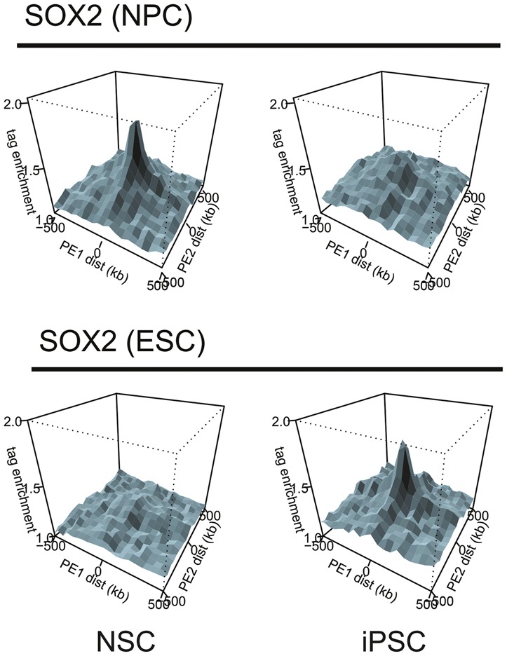
PE-SCAn to combine Hi-C and ChIP-seq data. A PE-SCAn (de Wit et al. 2013) analyzes whether sequences bound by a chromatin factor of interest show preferential long-distance (i.e., TAD-crossing) interactions. The depicted example is reprinted from Krijger et al. (2016) and shows the relationship of Sox2-binding profiles obtained in mESCs and mouse NPCs (neural progenitor cells) and the chromatin interactions detected in NSCs and iPSCs (induced pluripotent stem cells). Note that the Sox2-binding sites detected in ESCs exclusively cluster in iPSCs, whereas the binding sites found in NPCs cluster in NSCs.

Recent evidence also shows that sub-TADs can be forced to move to other nuclear subcompartments upon artificial recruitment of different chromatin factors, with, for example, the recruitment of the polycomb protein Ezh2 causing repositioning to a compartment with other polycomb-bound sub-TADs, and Suv39H1 dragging the sub-TAD from the A compartment to the B compartment (Wijchers et al. 2016). The latter appeared to depend on the chromodomain of Suv39H1, suggesting that nuclear compartmentalization can involve interactions between proteins bound to the one sub-TAD and histone modifications present at the other. Nuclear repositioning was uncoupled from gene regulation, as was also seen upon the targeted recruitment of a chromatin decondensing acidic peptide, which induced locus repositioning without changing the transcriptional output of the comigrating gene (Therizols et al. 2014). Together, these and other studies support the idea that multiple nuclear subcompartments exist that dynamically alter in composition during differentiation and reprogramming. The spatial aggregation of TADs and sub-TADs seems to have a contributory rather than a deterministic impact on gene expression.

CTCF- and cohesin-mediated architectural loops surrounding TADs

CTCF is a protein with insulator activity (Bell et al. 1999) that demarcates domains with distinct chromatin signatures (Cuddapah et al. 2009). It was one of the first factors established to be involved in chromatin looping (Splinter et al. 2006; Handoko et al. 2011), and recent studies have firmly established this protein and its functional partner, cohesin, as one of the main architectural players in mammals.

CTCF not only associates with but also positions the ring-shaped cohesin protein complex on chromatin (Koch et al. 2008; Parelho et al. 2008; Rubio et al. 2008). Hi-C studies demonstrated that CTCF is enriched at the boundaries of TADs (Dixon et al. 2012). Subsequent Hi-C studies of even higher resolution showed that, in fact, structural domains like TADs are part of encompassing chromatin loops, very often with CTCF at the anchors (Rao et al. 2014). The deletion of a boundary region at the X inactivation center led to partial fusion of the adjacent TADs (Nora et al. 2012). Similarly, deletion of CTCF-binding sites at one given TAD boundary caused active chromatin marks to enter a normally repressed domain (Narendra et al. 2015) and at another boundary caused gene dysregulation, presumably because of inadvertent interactions with regulatory elements in the neighboring domain (Dowen et al. 2014). A recent study investigating oncogene activation in IDH1 (isocitrate dehydrogenase 1) mutant gliomas showed that the CpG island methylator phenotype present in these tumors results in reduced binding of the methylation-sensitive CTCF protein to its (hypermethylated) binding sites. This weakened the domain boundaries and thereby caused aberrant enhancer–promoter interactions with glioma oncogenes (Flavahan et al. 2016). Depletion of cohesin or CTCF led to a decreased ratio of intra-TAD over inter-TAD contacts, indicative of boundary disruption (Seitan et al. 2013; Sofueva et al. 2013; Zuin et al. 2014). However, this occurred to different degrees for each of the two proteins, perhaps because of differences in depletion efficiency. The physiological relevance of boundaries segregating potential enhancer–promoter interactions was impressively demonstrated for the case of sporadically inherited limb malformations such as polydactyly. Deletions, inversions, or duplications across domain boundaries of the same locus caused different kinds of malformations in different families because each rearrangement brought a different gene under the control of the same limb regulatory landscape (Lupianez et al. 2015). Finally, recurrent microdeletions were recently found in T-cell acute lymphoblastic leukemia (T-ALL) that eliminate CTCF-mediated boundaries of domains containing prominent T-ALL proto-oncogenes. Using genome editing to recapitulate some of these deletions, (mild) up-regulation of the TAL1 and LMO2 oncogenes was observed and proposed to be the result of the release of enhancers from neighboring TADs (Hnisz et al. 2016). Collectively, these data affirm that domain boundaries formed by CTCF and its looping partner, cohesin, play a crucial role in the physical and functional segmentation of chromosomes through the formation of chromatin loops between cognate binding sites. These architectural loops ensure the correct wiring of enhancers to target genes and prevent inadvertent regulatory cross-talk across boundaries.

From a molecular perspective, one of the most striking observations made by high-resolution Hi-C was that CTCF-binding sites engaged in chromatin looping are nearly always in a convergent orientation. As the DNA recognition sequence of CTCF is not palindromic, it can be regarded as having a forward (F) or reverse (R) orientation, which implies that pairs of CTCF sites at the base of a loop theoretically can have four different relative orientations: FF, RR, FR, and RF (Rao et al. 2014). In line with the importance of relative CTCF-binding site orientation, motif orientation is often conserved among distinct species, particularly at conserved domain boundaries (Vietri Rudan et al. 2015), and boundaries often harbor pairs of divergently oriented CTCF-binding motifs (Gomez-Marin et al. 2015). Thanks to the advent of CRISPR/Cas9 genome editing, the observed dependence of CTCF-mediated looping on motif orientation could be validated. The deletion—but more interestingly, also the inversion—of CTCF-binding sites disrupted chromatin loops between originally convergently oriented sites, and, in some cases, this also led to the altered expression of nearby genes (Fig. 3; de Wit et al. 2015; Guo et al. 2015). An intriguing and currently debated issue is what the molecular mechanism may be that causes chromatin looping to selectively take place between distal convergently oriented CTCF sites. The extrusion model is favored. It proposes that DNA is actively extruded through cohesin rings until reaching two compatible roadblocks that stabilize the thereby formed chromatin loop (Fudenberg et al. 2015; Sanborn et al. 2015). For roadblocks to be compatible, it is assumed that CTCF molecules must be bound in a convergent orientation. Proteins with motor capacity, such as RNA polymerase, may facilitate extrusion (Dekker and Mirny 2016).

Figure 3.

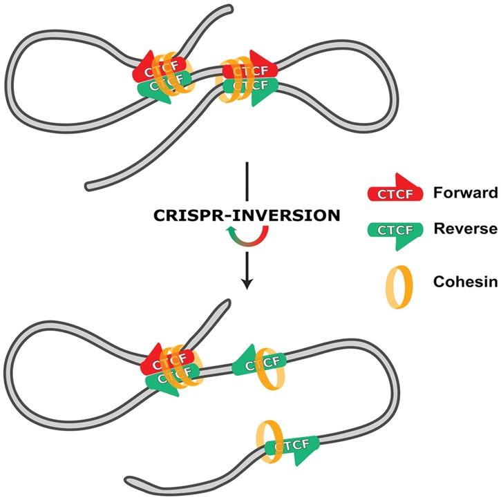
CTCF binding polarity determines chromatin looping. Convergently oriented CTCF-binding sites are found at the base of chromatin loops and recruit the additional architectural protein cohesin. Motif inversion using CRISPR impedes looping, with cohesin recruitment being unaltered. Gene expression can also be affected. (Reprinted from de Wit et al. 2015.)

Regulatory enhancer–promoter contacts

Original 3C studies applied to individual gene loci established the importance of enhancer–promoter contacts. The investigated loci showed that tissue-specific long-range regulatory interactions were absent in cells not expressing a particular gene, suggestive of a genome that dynamically changes conformation and regulatory contacts between cell types. Subsequently, however, tissue invariant regulatory interactions were also described that appeared to be present even when a particular gene was inactive (de Laat and Duboule 2013). An example of a tissue invariant or permissive configuration includes the Shh gene and its extensively characterized limb bud enhancer nearly 1 Mb away. Hi-C results established that the enhancer and gene coincided with the boundaries of a tissue invariant TAD (Dixon et al. 2012). Pre-existing loops were further described, for example, in p53- and TNFα-dependent transcriptional regulation (Jin et al. 2013; Melo et al. 2013) and the HoxD locus (Montavon et al. 2011).

The Hox genes, which contribute to the body plan during vertebrate development, provide a compelling example of expression control in 3D. Within the Hox gene clusters, Hox gene paralogs are arranged collinearly, with their order reflecting their relative spatial and temporal expression patterns. For the establishment of the body axis, the genes do not seem to rely on long-range DNA contacts. Rather, 4C revealed that, in time and space, the gene cluster gradually unfolds, adopting a bimodal architecture with a hub of active genes that is spatially segregated from, but gradually incorporates, a hub of inactive genes, concomitant with the spatiotemporal deposition of active histone modifications (Noordermeer et al. 2011b). A similar dynamic chromatin landscape has been described for the mouse HoxA cluster as well as the zebrafish Hox genes (Woltering et al. 2014). For establishment of the extremities, Hox gene regulation does rely on long-range regulatory contacts. During limb bud development, HoxD genes are expressed in two successive phases in a manner that depends on regulatory sequences present in the flanking gene deserts. A dynamic TAD border within the gene cluster ensures that, at the proper time and place, the relevant genes are exposed to either the digit enhancers located on the centromeric side or the forearm enhancers located on the opposite side (Andrey et al. 2013). Part of these long-range regulatory contacts, albeit reduced, appear pre-established, as they are found to also exist in unrelated tissue not expressing the Hox genes (Montavon et al. 2011).

The systematic mapping of chromatin loops across multiple cell types by high-resolution Hi-C provided a better understanding of the developmental dynamics of loop formation. Based on the analysis of nearly a billion Hi-C ligation junctions per cell type, ∼10,000 long-range contacts or loops (mostly between loci <2 Mb apart) were called per cell line (Rao et al. 2014). This is less than the 1 million contacts reported in another study (Jin et al. 2013), a discrepancy that seems attributable to differences in data analysis and peak calling, which defines contacts and loops. Approximately 30% of the 10,000 loops involved genes, which were, on average, more highly expressed (sixfold) than nonlooped genes in the same cell type. Roughly 25% of the gene loops were absent in a given other cell line, which concomitantly expressed these genes at much lower levels. Collectively, this supports the idea that, across the genome, gene looping contributes to higher expression levels (Rao et al. 2014). It also reveals that pre-established (permissive) and de novo established (instructive) chromatin loops coexist. We speculate that de novo established regulatory loops may be particularly relevant if genes must be expressed at high levels in a given cell type. How these loops relate to promoter–promoter contacts and enhancer hubs that have been observed by ChIA-PET studies against RNA polymerase II (Pol II) or enhancer-associated p300 (Li et al. 2012; Kuznetsova et al. 2015) remains to be determined. Using a modified ChIA-PET protocol optimized for long reads and monitoring both CTCF and Pol II interaction networks, “CTCF/cohesin foci” were described that also accumulate the transcriptional machinery (Heidari et al. 2014; Tang et al. 2015). In agreement, Hi-C also demonstrated that not only architectural loops but also gene-centered regulatory chromatin loops involve CTCF (Rao et al. 2014). Cohesin had already been reported before to frequently associate with looped enhancers (Kagey et al. 2010). Altogether, this suggests that it may be an oversimplification to classify loops as being either architectural or regulatory.

Direct evidence for the functional relevance of chromatin loops between distal enhancers and gene promoters was beautifully provided by experiments that artificially tethered gene promoters to a specific enhancer. Mutant erythroid cells lacking the transcription factor GATA1 do not form a chromatin loop between the globin genes and their upstream enhancer, the locus control region (LCR); correspondingly, the globin genes are expressed at low, basal levels. While GATA1 depletion abrogates binding of Ldb1 to the gene promoters, the Ldb1 complex is still recruited via other transcription factors to the LCR. Artificial recruitment of Ldb1 (or its self-association domain only) via an engineered zinc finger to the β-globin promoter appeared sufficient to not only re-establish the regulatory loop with the LCR but also strongly activate the recruited gene (Deng et al. 2012). This demonstrated that looping causally underlies gene activation. Importantly, the investigators found in a later study that they could also activate the developmentally silenced fetal γ-globin promoter by recruiting it to the LCR in primary adult human erythroblasts. Concomitantly, the adult β-globin gene reduced its contacts with the LCR and lowered its transcriptional output (Fig. 4; Deng et al. 2014). As the investigators speculated, redirecting the LCR from adult to fetal globin genes by forced looping holds therapeutic promise for sickle cell anemia and β-thalassemia patients who improperly express their adult β-globin genes.

Figure 4.

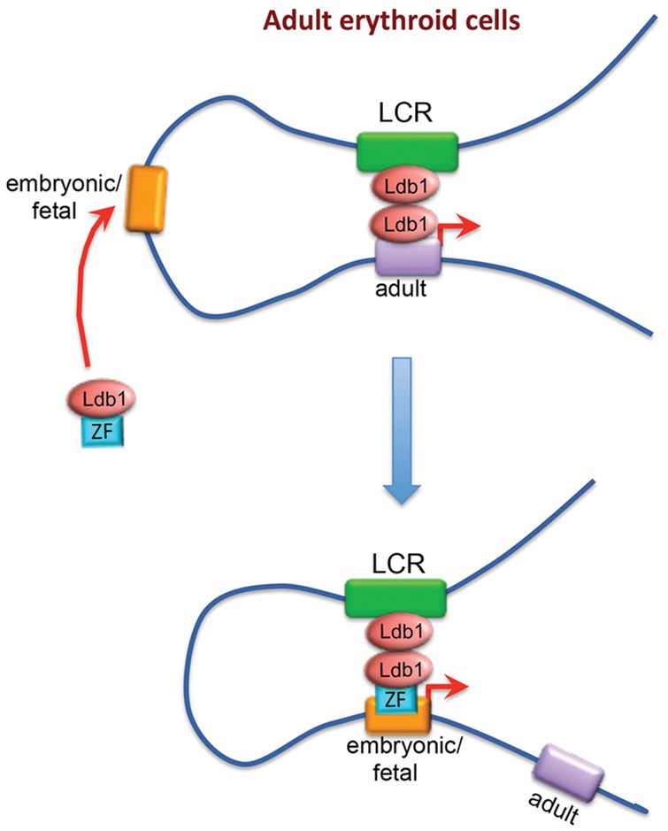
Manipulating chromatin looping in vivo. In both murine and human adult erythroblasts, the transcription cofactor Ldb1 can be recruited to the developmentally silenced embryonic or fetal β-globin promoter via a zinc finger (ZF). This results in increased interaction with the LCR at the expense of the adult globin genes and concomitant changes in gene expression. (Reprinted from Deng et al. 2014 with permission from Elsevier.)

Explaining disease in the 3D genome

A truly exciting breakthrough enabled by the availability of 3C technologies and our current understanding of gene regulation in 3D is our greatly improved ability to unveil the functional consequences of genetic variation. Compelling examples were recently published in which 3C studies decisively helped to unravel the molecular mechanisms underlying disease (Lupianez et al. 2016).

One such study involved the use of 4C technology to search for the mechanism by which recurrent inversions and translocations within chromosome 3 [inv(3)/t(3;3)] cause acute myeloid leukemia (AML). These rearrangements are associated with up-regulation of the stem cell regulator and proto-oncogene EVI1, which is located just outside the rearranged region. 4C showed that this up-regulation was due to ectopic interaction of the gene with an enhancer present in the inverted chromosomal segment. Indeed, knockout of this enhancer by genome editing reduced EVI1 oncogene expression in an AML patient cell line. At its endogenous location, 4C showed that this same enhancer normally interacts with the GATA2 tumor suppressor gene. Correspondingly, targeted deletion of this enhancer reduced GATA2 expression in wild-type cells (Groschel et al. 2014). EVI1 up-regulation and GATA2 haploinsufficiency independently are sufficient to drive leukemia, showing the dual impact of enhancer hijacking.

As referred to already, the study by Lupianez et al. (2015) provides another very nice example of how disease mechanisms unfold in the context of the 3D genome. There, different genomic rearrangements involving a number of neighboring TADs caused different types of limb malformations. The central TAD involved exclusively contains the EPHA4 gene, which is normally expressed in the developing limb bud. By applying 4C, it was demonstrated that, in each of the cases, different TAD boundaries were disrupted, placing a different gene (WNT6, IHH, or PAX3) under the control of the EPHA4 regulatory landscape and driving their ectopic limb expression. As in the AML study, hypotheses generated based on 4C contact maps were validated by genome-editing experiments, showing that boundary integrity is indeed crucial to prevent limb malformations due to ectopic activation of genes surrounding the EPHA4 TAD (Lupianez et al. 2015).

One of the earliest studies highlighting the benefits of topological analysis when aiming to uncover the relevance of genetic variation focused on a risk variant associated with skin pigmentation. Application of 3C technology demonstrated that the variant destabilized an enhancer–promoter loop with the OCA2 gene, leading to its down-regulation (Visser et al. 2012). At a genome-wide level, haplotype-resolved Hi-C-based contact maps enabled linking contact frequencies to allele-specific expression differences (Dixon et al. 2015). Implementing genome organization also helped to link risk variants associated with obesity to unanticipated target genes. Variants in introns of the FTO gene, a gene that can influence body mass in mice (Fischer et al. 2009), were found to be located within enhancers that regulate and contact the IRX3 and IRX5 genes, ∼0.5–1 Mb away from the variants (Smemo et al. 2014; Claussnitzer et al. 2015).

In summary, advances in 3C methodologies, increased resolution contact maps, and improved strategies for data analysis (discussed below) in the last years have led to a substantially enhanced understanding of genome structure. We now appreciate that chromosomes are subdivided into structural and functional units called TADs, with CTCF and cohesin being crucial actors at their boundaries. TADs limit the contact search space for sequences and thereby direct enhancers to genes that co-occupy the same TAD. Boundary integrity is crucial to prevent enhancer hijacking, which can lead to disease. While local enhancer–promoter contacts and TAD structures are the most important regulators of gene expression, TADs also organize themselves in nuclear compartments with defined chromatin signatures. However, these higher-order structures seem to have a contributory rather than a deterministic impact on transcription.

Below, we discuss newly emerging 3C technologies and highlight strategies to analyze 3C-based data. Finally, we present a scheme that we hope will help scientists decide which technology to choose for their specific research question.

Entering the stage: Capture-C approaches

For reasons explained above, we recommend using the more unbiased 4C or 5C approaches over classic 3C technology, but these technologies have their potential limitations. 4C, as discussed, is only semiquantitative. It can readily be applied to tens of sites simultaneously, but scaling up to analyze hundreds of genomic sites is very laborious. 5C depends on the use of six-cutters: Ordering all of the primers needed to benefit from the increased resolution provided by four-cutters would be prohibitively expensive. Thus, the necessary up-front investment in primers and the availability of Hi-C nowadays may be the reason why 5C appears to be not widely adopted. Hi-C is completely untargeted and ideally suited to obtaining a more general picture of genome folding. However, nowadays, the more exciting biology is often to be found only in detailed contact maps, which require extremely deep sequencing of Hi-C libraries. Also, if a research question is focused on a specific genomic site, a specific locus, or even specific categories of sequences (such as gene promoters, enhancers, boundaries, etc.), the great majority of Hi-C reads is superfluous, and the sequencing of Hi-C libraries therefore becomes prohibitively expensive. Recognizing these limitations, alternative strategies have been presented. They have in common that they employ the hybridization of oligonucleotide probes to selectively pull down ligation junctions of interest.

One such strategy was termed targeted chromatin capture (T2C) (Kolovos et al. 2014), which essentially offers an alternative to 5C technology. As depicted in Figure 2, the protocol basically follows standard 3C library preparation (using a six-cutter for the digest), but, instead of the sonication used in Hi-C protocols, T2C uses a second restriction digest with a four-cutter to fragment the library; sequencing adapters are then added via ligation. Prior to sequencing, the library is hybridized to custom-designed oligonucleotides specific to the region of interest. Since the biotinylated oligos can be immobilized on either a microarray or beads, this strategy enables targeted sequencing of contacts made by the sequences of interest. In the original study, T2C was employed to investigate the chromatin conformation of the well-studied mouse β-globin and human H19/IGF2 loci (Kolovos et al. 2014).

To monitor more distinct sites in parallel (i.e., a “many versus all” approach), others (Hughes et al. 2014) used the same concept of target enrichment but with a slightly different protocol (see Fig. 2): First, a four-cutter is used during 3C-seq library preparation. Second, sonication is employed rather than a second restriction digest. Third, biotinylated RNA baits are used in combination with streptavidin beads to pull down the regions of interest. Also here, the new method, termed Capture-C, was validated using the α-globin and β-globin loci. Capture-C was shown to be a useful technique to link single-nucleotide polymorphisms (SNPs) within regulatory sequences to the genes that they control. However, the data also showed that enrichment efficiency differed substantially between sequences of interest. Moreover, it was realized that, as in ChIA-PET, the interpretation of contact profiles within a locus of interest is compromised if the procedure enriches some sequences (to different degrees) but not others. These issues were addressed in an updated protocol published by the same investigators, termed NG Capture-C (Davies et al. 2016). First, instead of multiple overlapping oligos, the investigators employed single, 120-bp-long biotinylated DNA baits (instead of RNA) targeted to each end of a restriction fragment of interest. Per locus or genomic region, only one such fragment was selected, but, throughout the genome, multiple dispersed sequences of interest could be monitored in parallel. Probes were designed to include the restriction site, which increased the capture of informative fragments. In addition, the new protocol includes PCR amplification and a second round of hybridization to the baits, which, in the examples shown, increased the percentage of on-target reads to ∼50%.

The use of sonication instead of restriction digestion to fragment the 3C template is an important improvement of the protocol. Sonication is a random DNA fragmentation method: Two identical but independently obtained ligation junctions will therefore be fragmented at different positions on either side. By directing paired-end sequencing to these ends, one can discern PCR duplicates (identical ends) from independent ligation events (different ends). Thus, whereas 4C technology is semiquantitative, Capture-C based on sonication and probe hybridization is a quantitative method to measure contact frequencies. NG Capture-C was again tested on the extensively studied globin loci (Davies et al. 2016) and confirmed in a more quantitative manner the well-established gene enhancer loops previously described by 3C technology (Tolhuis et al. 2002) and 4C-seq (van de Werken et al. 2012b).

Several other studies have employed a variation of the Capture-C protocol. In one strategy, a six-cutter was used for the first digest, with a subsequent biotin fill-in and pull-down to enrich for ligation junctions, followed by further enrichment using capture probes. The biotin pull-down increased the signal to noise ratio (Jager et al. 2015), but this step may be omitted when employing two rounds of capture pull-down (Davies et al. 2016). Two studies employing this protocol queried the contact profiles of 22,000 promoters in either mESCs and mouse fetal liver cells (Schoenfelder et al. 2015) or two human blood cell types (Mifsud et al. 2015b). Distal elements contacting promoters could not only display enhancer marks when interacting with active genes but also bear repressive marks when contacting inactive genes, thereby possibly representing long-range silencers. In a method called HiCap, resolution was increased by using a four-cutter instead of a six-cutter to digest cross-linked chromatin, followed by promoter enrichment, which resulted in substantially higher resolution. When applied to ESCs, sites contacting promoters were found to be enriched for active enhancer marks (Sahlen et al. 2015).

An essentially similar approach employing a four-cutter to digest cross-linked chromatin but using probes directed to DNase I-hypersensitive sites (Joshi et al. 2015) confirmed the clustering of H3K27me3/polycomb-marked regions like the Hox gene clusters in ESCs (Denholtz et al. 2013; Vieux-Rochas et al. 2015). mESCs are known to exist in different states, with serum ESCs being more similar to post-implantation pluripotent stem cells and more developmentally primed than ground-state pluripotent 2i cultured ESCs. The study showed that these long-range intrachromosomal and interchromosomal contacts existed in serum mESCs but disappeared in a reversible manner in 2i mESCs. In primed ESCs, they were dependent on polycomb (Joshi et al. 2015). Finally, a “DNase Hi-C” protocol was introduced that uses DNase I treatment instead of restriction digest to fragment chromatin, with the advantage of smaller fragment sizes and the ability to filter out PCR duplicates (as described above for sonication). The strategy, called DNase Hi-C, was combined with DNA capture technology to direct contact analysis to nearly 100 promoters of long ncRNAs (lincRNAs). The study revealed complex transcriptional regulation by both superenhancers (clusters of enhancers occupied by an exceptionally high density of transcription factors) and PRC2 (Polycomb-repressive complex 2) (Ma et al. 2015).

In summary, the Capture-C method and its derivatives make up the newest members of the family of 3C-like technologies using capture probes to target contact analysis to selected sequences. As compared with Hi-C, they can offer the advantage of analyzing detailed genome-wide contact profiles of many loci in parallel while substantially reducing sequencing costs. As compared with 4C-seq, they may enable parallel analysis of many more sites of interest. The use of DNase instead of restriction enzymes for the fragmentation of cross-linked DNA (Ma et al. 2015) or the use of sonication for the fragmentation of the 3C template (Davies et al. 2016) can be advantageous as data interpretation becomes more quantitative: PCR duplicates can be discerned from independent ligation events and filtered out. Below, we provide considerations to help scientists select the 3C tool best tailored to their research question.

Choosing a 3C method for your research question

When deciding on the method of choice, aspects to consider include the required resolution of contact maps, the number of genomic sites that one wishes to interrogate, possible biases introduced by the selected method, ease, and costs.

No matter which 3C technology is chosen, it is important to maximally preserve the original 3D configuration until ligation has completed, as this ensures that as many ligation products as possible are a reflection of their original proximity in the cell nucleus. This was recently discussed in the context of Hi-C, as it was realized that the original Hi-C protocols yielded an unsatisfyingly high percentage of interchromosomal fusions (often 60%). An overrepresentation of interchromosomal fusions is typically expected to be due to random ligations between unrelated (i.e., uncross-linked) DNA fragments. While this does not devaluate the relevance of measured intrachromosomal contacts, particularly those measured over medium-range (<2 Mb) or short-range distances, it does reduce the percentage of informative read pairs and may obscure specific contacts over extremely long (>10 Mb) distances within and between chromosomes (Nagano et al. 2015). Signal to noise ratios were improved independently in 4C (Splinter et al. 2012) and Hi-C (Nagano et al. 2013; Rao et al. 2014) protocols by the omission of a sodium dodecyl sulfate (SDS)-mediated nuclear lysis step prior to ligation. In this modified procedure, ligation takes place in situ inside the nuclei instead of “in solution,” thereby decreasing the percentage of interchromosomal fusions to ≤20%, as determined by 4C-seq (van de Werken et al. 2012a) as well as Hi-C (Rao et al. 2014; Nagano et al. 2015). As such, these protocols acknowledge observations by others that dilution prior to ligation is not critical (Comet et al. 2011) and that the majority of cross-linked chromatin is not released from nuclei upon restriction digest and SDS treatment (Gavrilov et al. 2013), both suggesting that the insoluble fraction comprising intact nuclei may indeed be the actual source of the 3C signal. Ligation in the nucleus is therefore recommended for all 3C-based methods.

Formaldehyde fixation is a well-established approach that is also used in many other methods, such as imaging, and whose mode of action is, in principle, well understood (Orlando et al. 1997). However, the propensity to be cross-linked to DNA seems to differ between distinct proteins (for example, histones are readily cross-linked to DNA, but the lac repressor and NF-κB are not) (Solomon and Varshavsky 1985; Nowak et al. 2005). This could be a drawback for not only ChIA-PET but also the detection of protein-mediated loops by any of the other 3C-like methods. In addition, highly dynamic and fluctuating interactions, such as observed between regulatory elements of the X inactivation center (Giorgetti et al. 2014), might not be detected, as formaldehyde cross-linking is presumed to require a residence time of at least 5 sec (Schmiedeberg et al. 2009). In any case, one should be aware that small alterations in fixation conditions—i.e., formaldehyde concentration or fixation time—might influence cross-linking efficiencies and should therefore be standardized. Importantly, however, Rao et al. (2014) performed five of their in situ Hi-C experiments without formaldehyde fixation, which rendered the same robust peaks as with formaldehyde. Therefore, while biases introduced by the fixation procedure due to protein propensity to be cross-linked to DNA and due to the residence time of the respective factors could be envisioned, cross-linking generally enables capturing the spatially most proximal DNA sequences. This is evident from the fact that 4C and Hi-C contact profiles affirmatively follow contact behaviors predicted by polymer physics (Rippe 2001) and is also in line with the fact that DNA FISH generally successfully recapitulates contact profiles as detected by 3C-like technologies. Note, however, that discrepancies between results obtained by the two methodologies have also been reported under certain conditions (Williamson et al. 2014). While both procedures involve chemical fixation, it is not well understood whether these are related to the digestion or SDS treatment in the 3C protocol or, for example, the denaturing steps of FISH protocols, which distort nuclear structure.

Another general issue to consider is the meaning of quantitative contact measurements by 3C methodologies. Obviously, the more quantitatively ligation junctions can be assessed, the more accurate the measurements will be. However, what 3C, 4C, 5C, Hi-C, ChIA-PET, and Capture-C essentially do is measure ligation frequencies between cross-linked and fragmented DNA sequences. Ample validation studies by means of microscopy or, even better, genetics (e.g., deletions showing that two dispersed sequences also functionally communicate) have shown that ligation efficiencies can be taken as a proxy for contact frequencies—but not more than that! For sequences to participate in 3C contact profiles, they must (1) be cross-linkable, (2) have DNA ends available for ligation, and (3) outcompete other fragments in a cross-linked DNA–protein aggregate for ligation to a given sequence. All of this depends on size, chromatin composition, fixative, and duration and stringency of fixation (Dekker 2006; Simonis et al. 2007; Gavrilov et al. 2013). This is why 3C measurements, no matter how quantitatively they assess ligation frequencies, are not directly translatable into absolute in vivo contact frequencies.

Irrespective of these considerations, Hi-C is the method of choice to obtain a comprehensive overview of a cell's contactome. It is to be expected that, within the coming 5 years, detailed Hi-C based genome contact maps will become available for most of the frequently used cell lines, most mouse and also human tissues and organoids, and individual cell types. These 3D contact maps will serve as an invaluable source for the interpretation of epigenomics and transcriptome data obtained from the corresponding cells but also for the interpretation of disease-associated genetic variation. In cases where the 3D impact of a given trans-acting factor (a given protein or ncRNA) with ubiquitous binding sites across the genome is studied, a choice may be made between either Hi-C or ChIA-PET. A major advantage of Hi-C is that contact frequency measurements are not influenced by antibody pull-down efficiencies. Also, in Hi-C, contacts between binding sites are assessed in the context of all other contact frequencies, often a prerequisite to truly understand their significance. Finally, with Hi-C, contact frequencies can also be measured in the absence of the trans-acting factor—something that is inherently impossible by ChIA-PET. Medium-resolution Hi-C maps in wild-type and knockout/knockdown cells in combination with ChIP-seq-generated DNA-binding profiles have already been used to uncover roles of general chromatin architectural proteins like cohesin (Seitan et al. 2013; Sofueva et al. 2013), lamin A (McCord et al. 2013), and linker histone H1 (Geeven et al. 2015) in genome folding.

If contact analysis is to be directed to a large but defined series of sites (for example, to hundreds or thousands of promoters, enhancers, or binding sites of a factor of interest), one of the Capture-C variants may be the method of choice, as they can provide more detailed contact maps for these sites at lower sequencing costs as compared with Hi-C.

If one wishes to analyze the conformation of an entire locus (e.g., of one or more TADs) without a desire to focus only on contacts formed by a few of its sequences (gene promoter, enhancers, or boundaries), one can use 5C (Dostie et al. 2006) or the Capture-C variant T2C (Kolovos et al. 2014). Both protocols currently use six-cutters, but, for high-resolution contact maps, we recommend using four-cutters or DNase I (Ma et al. 2015) to fragment cross-linked chromatin.

In Capture-C methods, biases to be aware of are differences in capture efficiencies between sites and overrepresentation of ligations between independently captured sites inherent to the method. Furthermore, as with 4C methods, care must be taken to include sufficient genome equivalents in the analysis in order to not produce anecdotal, nonreproducible contact profiles. Finally, capture probe libraries, but also 5C primer libraries, are not cheap. With the ever-dropping sequencing costs, one should therefore ask per project whether the Capture-C or 5C method of choice is indeed more cost-effective than Hi-C. If not, we recommend using Hi-C, as the data are less susceptible to technical biases and therefore are easier to interpret.

When the research interest concerns only a single or a few (up to several tens) genomic sites (as would be the scenario when studying the impact of a given rearrangement, genetic variant, gene promoter, or CRISPR–Cas-modified site), 4C-seq (van de Werken et al. 2012b) or NG Capture-C (Davies et al. 2016) can be used. Provided that both methods identify the same contacting sites, as evidence so far suggests, NG Capture-C may be preferred if the exact quantification of ligation events is deemed beneficial. Alternatively, 4C-seq may offer an arguably easier to implement, but certainly cheaper, method proven to detect the relevant contacts. Costs of two large 120-bp biotinylated capture probes, two rounds of PCR, a hybridization kit, and an Illumina library preparation kit plus the inefficient sequencing (at least 50% off-target) involved in NG Capture-C (Davies et al. 2016) need to be compared with the costs of two ready-for-sequencing 80-mers that require a single round of PCR to prepare a sequencing library with nearly 100% of the reads on target. Again, for both methods to produce meaningful results, library complexity is crucial: Analysis is therefore preferably directed to at least 10,000 genome equivalents.

Computational aspects of 3C methods

A recent breakthrough is that tools and packages are now becoming available for the analysis of data generated by the various 3C methods. The basic steps in the analysis of experimental data obtained by 3C-like methods are mapping of the reads, quality control, filtering, normalization, peak calling, and visualization of results. It is beyond the scope of this review to discuss data analysis in detail; for excellent reviews on the topic, we refer to Dekker et al. (2013), Ay and Noble (2015), and Lajoie et al. (2015). Here, we limit ourselves to summarizing some critical considerations relevant to the analysis and interpretation of results. We give a short and by no means exhaustive overview of publicly available packages and pipelines tailored at either some or all of these steps. As pointed out in these reviews, with all of the different packages available now, the development and general application of standardized and transparent analysis procedures will be necessary to ensure comparability between different studies.

Data interpretation

An issue to keep in mind when interpreting 3C-derived data is that identical cells have different 3D genomes even when synchronized in the cell cycle. This is because genome folding is highly probabilistic (Nagano et al. 2013; Kind and van Steensel 2014), particularly at the higher-order levels of 3D organization (nuclear positioning of TADs in the A and B compartments and/or relative to the periphery) (Gibcus and Dekker 2013; Krijger and de Laat 2013). 3C protocols render only an average view of genome conformation within a population of cells. Appreciable contacts can therefore be rare in terms of penetrance throughout the population and in time. Also, if contact profiles reveal multiple interactions from the same viewpoint, these may well represent distinct chromatin conformations found within various subpopulations. Finally, it should be realized that even stable and reproducible contacts do not necessarily reflect biological function. 3C technologies only measure physical proximity, and experimental genome editing or naturally occurring genetic variation is necessary to uncover the functional relevance of chromatin contacts.

Data quality should be carefully assessed prior to interpretation. As alluded to, assessing the intrachromosomal over interchromosomal ratio is informative in this respect: High-quality 4C, Capture-C, and Hi-C data sets tend to have ≤20% trans captures. If more abundant, results are likely noisier, but this does not imply that the local intrachromosomal contact profiles extracted from the same data are not informative. For 4C using four-cutters, we also routinely check the percentage of captured frag-ends in a 200-kb window around the viewpoint (±100 kb). When ≥80%, libraries are considered complex and suitable for contact analysis (van de Werken et al. 2012a). Note further that in both 4C and Hi-C, it is normal that ∼20% of the reads represent “undigested” or “self-ligated” products (van de Werken et al. 2012a). In the former case, the first restriction enzyme did not cut this specific site, or the induced cut immediately religated so that neighboring genomic fragments remain fused. “Self-ligated,” on the other hand, refers to circularization of the viewpoint fragment. In preparation for analysis, we routinely remove these undigested and self-ligated products from the data.

To identify significant interactions, the observed coverage in a given genomic region needs to be compared with a background model of expected coverage. Very high coverage is expected in close proximity to a given sequence, but this decreases rapidly with increased site separation. Single ligation events are either too rare (Hi-C) and/or may be too prone to experimental biases in cross-linking, ligation, or amplification efficiencies to be interpreted independently. Also, if two sites loop to each other, they necessarily drag along their immediate neighboring sequences, which can then also participate in cross-linking. To account for this, running window approaches are often used to smoothen and analyze the data. To subsequently interpret the observed signal in a given window, background models are needed for comparison. These models may differ between various analysis packages.

Data analysis: 4C analysis packages

The R package FourCSeq is a pipeline that is increasingly used for end-to-end analysis and peak calling of 4C data (Klein et al. 2015). Prior to fitting the background model, the observed 4C counts are normalized using a variance-stabilizing transformation to reduce the different levels of noise given by counts coming from low- and high-abundance fragments. The pipeline employs a monotonically decreasing model to fit the data to reflect the distance-dependent signal decay. The user can choose to either assume symmetric decay around the viewpoint or perform monotonic regression on both sides of the viewpoint separately.

To determine differential contacts between experimental conditions or cell types, the DESeq2 package (adapted from RNA sequencing [RNA-seq] analysis) can be employed (Love et al. 2014). We recently developed a similar peak-calling algorithm, which also fits a monotonically decreasing model to the data using isotonic regression (de Wit et al. 2015). This algorithm models the two sides of the viewpoint separately to account for local differences in background signal distribution. This seems relevant to most bait sequences, especially when close to TAD borders. To robustly identify loci of increased contact frequency, we employ repeated subsampling to mitigate the effect of outliers and define stringent criteria for peak calling. Using this analysis pipeline, we identify fewer contacts than FourCSeq, which, by extrapolation, better agree with the number of loops identified in high-resolution Hi-C (Rao et al. 2014).

For the visualization of 4C results, several graphical approaches are available (see Fig. 5). One may choose one of the genome browsers for visualization of the running window graphs, which is especially informative if one is interested in local topology. Overlays of multiple normalized contact plots can help to visually emphasize differences in contact frequencies as induced, for example, by site-specific recruitment of certain trans-acting factors (Wijchers et al. 2016). For chromosome-wide contacts, for example, between TADs co-occupying the A (or B) compartment, arachnograms may be intuitive, as they depict the viewpoint as the origin for several branches (or “spider legs”) toward the contacted loci. A corresponding means to visualize interchromosomal contacts are Circos plots, which depict the whole genome as a circle (Krzywinski et al. 2009). Finally, a more quantitative approach would be domainograms, which employ a color scale to depict the significance of a contact across a range of differently sized windows (de Wit et al. 2008). R scripts and example files for these analyses can be found in Splinter et al. (2012).

Figure 5.

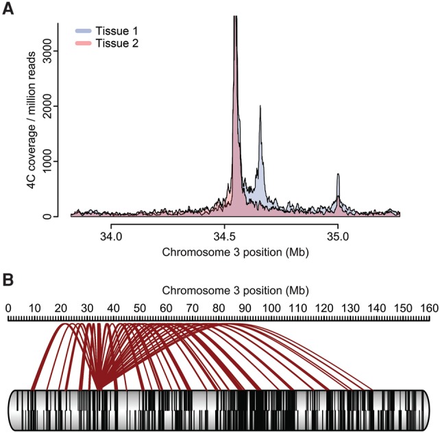
Visualizing 4C data. (A) Especially when interested in local contact profiles, a coverage plot representation of the normalized 4C data may be chosen. Data are from the same locus as the 4C plot in Figure 1. The panel depicts an overlay of contact profiles from two tissues (depicted in blue and orange). An overlay is shown as dark red. (B) Alternatively and when depicting long-range contacts, a “spider plot” or arachnogram can be employed. Contacts from the viewpoint to other regions on the cis chromosome are depicted in brown. Black lines within the chromosome represent genes.

Hi-C data analysis

While Hi-C libraries are sequenced paired-end, one needs to map both ends separately to the reference genome, as the two ends should represent two distant loci. However, one needs to decide how to handle chimeric reads; i.e., cases in which a read from one end already runs into a ligation junction sequence so that this read basically represents two genomic fragments. One strategy to resolve this issue is iterative mapping, in which each read is first truncated to 25 bp (starting at the 5′ end), mapped, and extended by 5 bp if not yet uniquely mappable (Imakaev et al. 2012). The process is repeated until either all reads could be uniquely mapped or the reads have been fully extended. Other approaches include pretruncation of reads containing potential ligation junctions (as used by the HiCUP pipeline, http://www.bioinformatics.babraham.ac.uk/projects/hicup) or performing a first mapping attempt followed by splitting of nonmapped reads at the ligation site and subsequently independently remapping the two pieces.

As a next step, the mapped reads should be filtered to ensure that only informative and reliable read pairs proceed to further analysis. For example, reads of low mapping quality should be removed as well as reads that do not agree with the size selection performed during the Hi-C library preparation. As for 4C, undigested and self-ligated fragments (read pairs coming from the same fragment) can be removed at this point. One method to achieve the latter is to simply perform a distance filter and further consider only pairs above a certain distance threshold. PCR duplicates should also be filtered out at this step.

After filtering, read pairs are binned to smoothen the data and increase the signal to noise ratio. Bins are either of a fixed genomic size or restriction fragment-based (analysis with multiple bin sizes could also be performed). The contact count for each bin pair is represented in a symmetric matrix. Before proceeding to normalization of observed counts, it can be advisable to remove bin outliers, which display a very low or noisy signal and often correspond to regions of the genome that are notoriously difficult to map, such as repetitive regions (e.g., centromeres and telomeres). For example, a cutoff for the bins with the lowest signal or highest variance can be applied.

For Hi-C data normalization, either an explicit or an implicit approach may be chosen (Ay and Noble 2015; Lajoie et al. 2015). In the explicit approach, a priori knowledge about technical and biological factors that can cause bias is required. Yaffe and Tanay (2011) developed a probabilistic background model to account for factors such as GC content, sequence uniqueness (i.e., mappability), and restriction fragment length. HiCNorm represents a simplified and therefore faster normalization procedure for the removal of systemic biases (Hu et al. 2012).

The implicit or matrix-balancing approach does not require definition of predetermined factors that may introduce bias. Instead, it is based on the assumption that, in an unbiased Hi-C matrix, all observed marginals have the same expectation (“equal visibility”). Imakaev et al. (2012) introduced an iterative correction and eigenvector (ICE) decomposition approach. ICE is based on alternating attempts to equalize the sums of matrix rows and matrix columns by dividing each row or column by its respective mean. Note that a faster balancing algorithm (Knight and Ruiz 2013) was recently employed for high-resolution Hi-C data (Rao et al. 2014). While the implicit approach has the advantage of correcting for not only known biases but also biases of unknown source, the assumption that all genomic regions should be equally represented in the matrix does not necessarily hold true; i.e., regions could be inherently difficult to map or reluctant to engage in long-range interactions (Ay and Noble 2015). No matter whether the explicit or the implicit approach is chosen, successful normalization should result in smoothened contact maps so that interactions are more easily identified.

After normalization, informative interaction patterns need to be extracted from the contact matrix. The first large-scale patterns to be extracted are the cell-specific A and B compartments that we described above (Lieberman-Aiden et al. 2009). These are generally relatively straightforward to identify, as they appear as a “checkerboard” pattern within the correlation matrix and are usually well captured by the first eigenvector in a principal component analysis.

As the next level of organization, TADs can be appreciated in the interaction matrix. These appear as smaller squares of increased interaction frequency along the diagonal. However, it should be noted that identification can be complicated by the complex and dynamic genomic organization into domains and subdomains. How can TAD boundaries be extracted computationally from a Hi-C data set? As explained by Lajoie et al. (2015), the general approach is to transform the Hi-C counts into some one-dimensional “insulation” statistic that captures the feature that characterizes domain boundaries. Note that TADs are defined as domains of increased self-interaction frequencies and that TAD borders are therefore naturally devoid of contacts crossing over them. Hence, an easy way to determine the domain association for a given locus or bin is to determine the ratio between its average upstream and downstream contacts, as has been done for mitotic chromosomes (Naumova et al. 2013). In a similar approach, Dixon et al. (2012) determined the locus-specific bias in upstream and downstream contacts and transformed this into a directionality index, which is expected to change sign at opposite sides of TAD boundaries. A hidden Markov model (HMM) is subsequently employed to call TADs (Dixon et al. 2012). An alternative approach is to first define TAD borders as bins with very few crossing contacts. This concept underlies approaches using a distance-scaling factor (Sexton et al. 2012) and the insulation score (Barutcu et al. 2015). Note that the former will be high at TAD boundaries, whereas the latter is minimal at boundaries. In addition, to identify sub-TADs, an “arrowhead” transformation can be applied to the Hi-C contact map, which results in arrowhead-resembling features representing domain corners, which then can be quantified using a “corner score” (Rao et al. 2014).

Paired-end spatial chromatin analysis (PE-SCAn) is a computational method that intersects Hi-C data with ChIP-seq data to search for preferred clustering of TADs enriched in binding sites of a given trans-acting factor of interest (de Wit et al. 2013). Using PE-SCAn, it was found that chromosomal regions that accumulate cellular identity factors such the pluripotency factors Nanog, Oct4, and Sox2 or the B-cell identity factor PU-1 cluster specifically in the corresponding cell types (Fig. 6; de Wit et al. 2013; Krijger et al. 2016).

Especially due to the resolutions achievable today, Hi-C maps not only provide large scale information about compartments and domains but can also detect loops between specific loci. As for 4C data, the challenge is to distinguish true contacts from noise and define a background model that suitably represents the background frequency of interaction between pairs of loci in the absence of specific interactions. This is challenging for intrachromosomal interactions, where the detected signal has to be evaluated in the context of the distance-dependent signal decay described above. Several different approaches have been used to obtain background models. For example, one can perform a parametric fit to best describe the data or bin all pairs of loci with the same genomic distance and then, for example, compute a P-value comparing the observed count for a given contact as compared with all other possible interactions in that bin (Duan et al. 2010). Background models can also take additional biases such as domain organization into account (as done by the HOMER software, http://homer.salk.edu/homer/interactions; see below). In comparison with these approaches, the HiCCUPS method calls peaks more stringently. HiCCUPS compares the counts obtained for a given matrix pixel with the surrounding regions (note, however, that this is computationally expensive) (Rao et al. 2014).

A means to follow the overall structural dynamics of chromatin looping between cell types is provided by Hi-C metaloop analysis. In this analysis, a given Hi-C data set is aligned on the loop calling data from another Hi-C data set. Data are then scaled between the beginning and end of each loop and projected on top of each other. By applying this strategy, it was shown that tissue-specific chromatin loops are effectively erased during cellular reprogramming of four different primary cell types (Krijger et al. 2016). In a parallel study that involved reprogramming of in vitro generated NPCs, incomplete re-establishment of the pluripotent 3D genome and persistent cell of origin-specific chromatin contacts were observed that could be linked to inaccurately reprogrammed gene expression. These features were abolished when cells were forced into a naïve pluripotency state (Beagan et al. 2016).

Hi-C analysis packages

An overview, by no means complete, of the available software tools for Hi-C data analysis that perform some or all of the above-mentioned steps is provided below. A more extensive summary of tools and packages can be found in Ay and Noble (2015) and at the very helpful Web site http://omictools.com/3c-4c-5c-hi-c-chia-pet-category.

HiC-Pro

HiC-Pro is a recently introduced pipeline that processes Hi-C data from raw reads to normalized matrices (https://github.com/nservant/HiC-Pro) (Servant et al. 2015). It contains a fast and memory-efficient implementation of the iterative correction procedure described above (Imakaev et al. 2012) and can build allele-specific contact maps if phased genotypes are available.

HiCUP

HiCUP (Servant et al. 2015) is a pipeline that maps the reads to the reference genome and removes artifacts such as religations as well as duplicate reads (http://www.bioinformatics.babraham.ac.uk/projects/hicup). It has also been used for capture Hi-C (Chi-C) experiments (see also the CHiCAGO pipeline, which employs a novel background correction procedure to robustly detect contacts specifically in capture-type Hi-C data, http://regulatorygenomicsgroup.org/chicago) (Cairns et al. 2015). The output obtained from HiCUP may then be used as input for other algorithms such as the Bioconductor package GOTHiC, which calls significantly contacting regions by employing a cumulative binomial test based on coverage (as it is assumed that biases are reflected in coverage) (http://master.bioconductor.org/packages/release/bioc/html/GOTHiC.html; Mifsud et al. 2015a).

HOMER

Another widely used software package that can use the output of HiCUP or any other mapping package to perform normalization and visualization is HOMER (note, however, that it does not perform bias correction) (http://homer.salk.edu/homer/interactions; based on Lieberman-Aiden et al. 2009). HOMER creates background models and contact matrices, normalizes counts, and identifies significant interactions. It encompasses several helpful programs, for example, to detect the above-described patterns such as compartments and compare Hi-C experiments. While HOMER has been tailored for the analysis of Hi-C data, it can also perform other tasks such as motif discovery. Overall, it is a very versatile tool package, specifically recommended for researchers without advanced knowledge of R.

Juicer

Juicer is a recently introduced new end-to-end pipeline (http://aidenlab.org/juicer). Juicer converts raw reads into Hi-C maps, which can be subsequently investigated and visualized in Juicebox (Rao et al. 2014), a flexible and user-friendly tool for browsing Hi-C data as well as domain calls, loops, and CTCF-binding sites (http://www.aidenlab.org/juicebox).

Modeling the 3D genome

To intuitively appreciate the 3D organization of single chromosomes or whole genomes, it would of course be desirable to transform chromatin conformation data sets into 3D models, similar to protein structures. To conclude the chapter on data analysis, we therefore want to give a few examples of recent attempts to model the 3D genome.

There are basically two different computational approaches for 3D modeling: using simulations of polymer physics, an approach that has been referred to as “direct,” as it does not rely on indirect methods such as chromatin conformation capture, and the “inverse,” or restraint-based approach, in which interaction probabilities derived from chromatin contact maps are used as restraints that are implemented in a scoring function, thereby basically constituting a computational optimization approach (Rosa and Zimmer 2014). These two separate approaches are explained in detail by Dekker et al. (2013), Ay and Noble (2015), and Serra et al. (2015). Explaining the physical details underlying polymer simulations is beyond the scope of this review; we therefore only want to provide a few examples illustrating the two major strategies that have been employed in restraint-based modeling.

As explained by Ay and Noble (2015) and Lajoie et al. (2015), restraint-based modeling can be further divided into two approaches: One attempts to identify either a consensus structure or an ensemble of structures that together satisfy the restraints and optimize the scoring function.

The consensus approach is more straightforward in that it ignores the fact that contacts detected by 3C-like methods represent bulk populations so that the contact matrices obtained are a mixture of different conformations present at variable frequencies. The biological relevance of such a consensus structure may therefore be debatable. To obtain a consensus structure, the classical statistical method multidimensional scaling is often employed, sometimes with additional constraints. For example, the approach has been applied to model the 3D organization of the budding and fission yeast genomes, and the models agreed well with the previously known clustering of centromeres in these eukaryotes (Duan et al. 2010; Tanizawa et al. 2010). Additionally, 3D genome models have been constructed for three time points in the life cycle of the malaria parasite Plasmodium falciparum (Ay et al. 2014) and for mESCs, with the latter employing a Bayesian method termed BACH (Bayesian 3D constructor for Hi-C data).

In a variant of the BACH algorithm, named BACH-MIX, structural variations of chromatin are modeled (Hu et al. 2013). Such an ensemble approach, which assumes that a collection of chromatin structures present in the population can best explain the contact frequencies as given by the Hi-C matrix, will reflect the underlying biology substantially better than the consensus approach but is naturally more complex. Another example for the application of the ensemble approach is a study in which a single optimization was used to derive thousands of genomic structures for a human lymphoblastoid cell line (Kalhor et al. 2012).

Tools for visualization of the derived 3D models are currently being developed. A scalable desktop application, GMOL, was recently presented (Nowotny et al. 2016), and a novel software tool named MOGEN for transforming chromatin conformation capture data into (ensemble) 3D models has recently been introduced (Trieu and Cheng 2016).

3C-type methods for rearrangement detection, genome assembly, and haplotyping

While 3C and its derivative methods were originally devised to shed light on the 3D organization of individual loci and whole genomes, the data obtained by these techniques were shown to also be of use for the analysis of the linear DNA scaffold. 3C-derived methods are applicable for the detection of chromosomal rearrangements, genome sequencing, assembly, and haplotyping as well as targeted gene sequencing, as discussed below.

Based on the theory that, irrespective of topology, sequences close together on the linear chromosomal template contact each other much more frequently than distal sequences, combined with proof thereof based on first 4C contact profiles, it was realized that 3C technologies can be highly informative to study chromosome scaffolds. When applied to samples from children with leukemia and directed to recurrently rearranged loci, 4C was found to robustly identify translocations and large inversions. Its capacity to search for them in an unbiased manner enabled the discovery of new oncogenes involved in leukemia (Simonis et al. 2009; Homminga et al. 2011). Based on these same principles that sequences located in cis (on the same chromosome) have a higher tendency to interact than sequences in trans and that proximal regions have a higher propensity to be in contact with each other than distal regions, different groups began to use Hi-C for contig assembly (Burton et al. 2013; Kaplan and Dekker 2013). An independent and, at least in terms of accounting for duplications, improved computational approach for Hi-C-based scaffold analysis, termed GRAAL (genome [re]assembly assessing likelihood), has recently been described (Marie-Nelly et al. 2014a).

Similarly, 3C-type data were used to fill annotation gaps in the yeast genome and determine the coordinates of difficult-to-map elements—such as origins of replication, centromeres, and noncoding functional elements of the genome such as centromeres and ribosomal DNA—based on their known tendency to cluster (Marie-Nelly et al. 2014b; Varoquaux et al. 2015).

A variant of the described 3C-derived assembly approach is the “Chicago” method (not to be confused with the CHiCAGO pipeline by Cairns et al. 2015; see above), which uses in vitro assembled chromatin for Hi-C library preparation (Putnam et al. 2016). Additionally, there is the arising application to metagenomics: When sequencing multiple species in a microbiome sample, it can be difficult to determine which contig belongs to which genome. However, by taking advantage of the fact that contigs from the same cell naturally have a higher contact probability than contigs originating from different cells, sequences from different species can be separated (Beitel et al. 2014; Burton et al. 2014). The transfer of mobile DNA elements such as plasmids through the population could also be followed, which can be instrumental in understanding the acquisition of antibiotic resistance in microbial populations (Beitel et al. 2014).

A second important application of 3C-type methods that is not directly related to 3D structure is haplotyping. Knowing the haplotype can be medically relevant, for example, to associate SNPs identified in GWAS (genome-wide association study) with driver genes or regulatory regions. Haplotyping is also important to understand human population histories and evolutionary genetics (for example, see Sabeti et al. 2007).

However, haplotyping is not a trivial exercise, and previous attempts to produce whole-chromosome haplotypes were generally technically difficult and required special equipment: For example, single chromosomes were obtained by FACS (fluorescence-activated cell sorting) (Yang et al. 2011), microdissection (Ma et al. 2010), or microfluidic separation (Fan et al. 2011). As an alternative, HaploSeq was introduced (Selvaraj et al. 2013), which takes advantage of the fact that chromosomes do not intermingle in the nucleus but occupy separate territories. Physically linked variants are therefore more likely to occur on the same rather than homologous chromosomes. The HaploSeq approach uses a modified version of the previously described HapCUT algorithm (Bansal and Bafna 2008) to build haplotype blocks from Hi-C data. A targeted version thereof for the resequencing, scaffolding, and haplotyping of selected loci is called targeted locus amplification (TLA). In sample preparation, TLA is comparable with the original 4C approach but with critical adaptations such that not only contact frequencies can be measured but the entire sequence of a locus can be reconstructed based on proximity ligation. TLA can be used to resequence genes and detect variants and rearrangements, gene fusions, and transgene or virus integration sites in an allele-specific manner (de Vree et al. 2014).

Future perspective

As presented in this review, the last years have seen exciting and unprecedented developments in the chromatin structure field in terms of both novel 3C-type methods and increased biological knowledge: Thanks to the ever-better resolutions achieved, we discovered first that the genome consists of TADs (which seem to serve as both structural and functional modules) and by now have gained an understanding that even these domains can be further divided into sub-TADs. We have started to understand the rules that govern changes in their nuclear positioning during development and the functional significance thereof. The dynamics and the factors responsible for architectural and functional chromatin loops are being uncovered. Genome-editing experiments now enable us to not only look for correlations but also perform the sort of cause and consequence experiments that are needed to fully understand whether and how genome folding impacts on DNA metabolic processes such as gene expression, replication, and DNA repair. With all of the novel chromatin conformation protocols, such as Capture-C and variations thereof, as well as the respective analysis pipelines accompanying nearly every newly published study, it will be important to streamline the approaches taken in the field as well as the terminology.

Of course, several technical advances would still be desirable and are currently being actively pursued. For example, simultaneously detecting multiway contacts to investigate whether chromatin hubs exist would render exciting new insights. Two recent studies provided proof of principle for multiway contact monitoring using either an in-gel replication approach (Gavrilov et al. 2014) or an assay termed tethered multiple 3C (TM3C), in which ligation is performed on agarose gel beads, and read pairs are decomposed to extract three-way ligations (Ay and Noble 2015). Such approaches should now be followed more systematically. Single-cell Hi-C, as was recently described by Nagano et al. (2013), will also be of special importance for evaluating the frequency of specific chromatin contacts within a cell population and cell-to-cell differences in genome folding during cell cycle progression and development. This first study showed that domains are rather conserved at the single-cell level but that interdomain contacts are highly variable.

In parallel to the development of techniques such as high-resolution Hi-C and Capture-C, our understanding of chromatin structure was, of course, also boosted by numerous novel imaging approaches, which we could not discuss here, as they were not the major focus of this review. However, a very informative review on this subject was published last year (Bystricky 2015). Here we only want to point out that, while FISH is a major tool to visualize genomic structure, live-cell imaging is needed to follow chromatin dynamics over time (basically in four dimensions). Nowadays, many more methods than integrating and tagging arrays of bacterial operator sequences (tetO and lacO) (Belmont and Straight 1998) are available for visualization. While some methods still require manipulation of the genomic sequence (Saad et al. 2014), other novel methods employ fluorescent proteins fused to transcription activator-like effectors (TALEs) (Ma et al. 2013; Miyanari et al. 2013), dCas9 (Chen et al. 2013), or even guide RNAs using aptamer sequences (Shao et al. 2016). A different approach is the m⁶A-Tracer that detects the adenine-6 methylation deposited by DNA adenine methyltransferase identification (DamID) (Kind et al. 2013). We anticipate that further exciting advances are to be expected in the areas of single-molecule live-cell imaging (for example, see Cisse et al. 2013) and high-throughput imaging (Shachar et al. 2015).

Of course and above all, a seemingly endless list of questions remains to be addressed until we can hope to better understand the functioning of the nucleus, the cell's major control unit; for example: Are genes in TADs indeed coregulated and, if so, to what extent? Which dynamics govern chromatin contacts? How are pre-established loops maintained in nonexpressing cells? What are the functional implications of pre-established versus de novo formed chromatin loops? What role do ncRNAs play in establishing and maintaining genome organization (Cech and Steitz 2014; Hacisuleyman et al. 2014; Quinodoz and Guttman 2014; Rinn and Guttman 2014)?

Answering these questions will require interdisciplinary approaches, easy-to-use and freely available analysis tools, and integration of data from both chromatin conformation methods and imaging techniques. Additionally, as discussed, we expect that 3D genome maps will increasingly be recognized as important for the interpretation of naturally occurring and disease-associated genetic variation. Clearly, an exciting decade still lies ahead.

References

- Andrey G, Montavon T, Mascrez B, Gonzalez F, Noordermeer D, Leleu M, Trono D, Spitz F, Duboule D. 2013. A switch between topological domains underlies HoxD genes collinearity in mouse limbs. Science 340: 1234167. [DOI] [PubMed] [Google Scholar]
- Ay F, Noble WS. 2015. Analysis methods for studying the 3D architecture of the genome. Genome Biol 16: 183. [DOI] [PMC free article] [PubMed] [Google Scholar]
- Ay F, Bunnik EM, Varoquaux N, Bol SM, Prudhomme J, Vert JP, Noble WS, Le Roch KG. 2014. Three-dimensional modeling of the P. falciparum genome during the erythrocytic cycle reveals a strong connection between genome architecture and gene expression. Genome Res 24: 974–988. [DOI] [PMC free article] [PubMed] [Google Scholar]
- Bansal V, Bafna V. 2008. HapCUT: an efficient and accurate algorithm for the haplotype assembly problem. Bioinformatics 24: i153–i159. [DOI] [PubMed] [Google Scholar]
- Barutcu AR, Lajoie BR, McCord RP, Tye CE, Hong D, Messier TL, Browne G, van Wijnen AJ, Lian JB, Stein JL, et al. 2015. Chromatin interaction analysis reveals changes in small chromosome and telomere clustering between epithelial and breast cancer cells. Genome Biol 16: 214. [DOI] [PMC free article] [PubMed] [Google Scholar]
- Bau D, Sanyal A, Lajoie BR, Capriotti E, Byron M, Lawrence JB, Dekker J, Marti-Renom MA. 2011. The three-dimensional folding of the α-globin gene domain reveals formation of chromatin globules. Nat Struct Mol Biol 18: 107–114. [DOI] [PMC free article] [PubMed] [Google Scholar]
- Beagan JA, Gilgenast TG, Kim J, Plona Z, Norton HK, Hu G, Hsu SC, Shields EJ, Lyu X, Apostolou E, et al. 2016. Local genome topology can exhibit an incompletely rewired 3D-folding state during somatic cell reprogramming. Cell Stem Cell 18: 611–624. [DOI] [PMC free article] [PubMed] [Google Scholar]
- Beitel CW, Froenicke L, Lang JM, Korf IF, Michelmore RW, Eisen JA, Darling AE. 2014. Strain- and plasmid-level deconvolution of a synthetic metagenome by sequencing proximity ligation products. PeerJ 2: e415. [DOI] [PMC free article] [PubMed] [Google Scholar]
- Bell AC, Felsenfeld G. 2000. Methylation of a CTCF-dependent boundary controls imprinted expression of the Igf2 gene. Nature 405: 482–485. [DOI] [PubMed] [Google Scholar]
- Bell AC, West AG, Felsenfeld G. 1999. The protein CTCF is required for the enhancer blocking activity of vertebrate insulators. Cell 98: 387–396. [DOI] [PubMed] [Google Scholar]
- Belmont AS, Straight AF. 1998. In vivo visualization of chromosomes using lac operator-repressor binding. Trends Cell Biol 8: 121–124. [DOI] [PubMed] [Google Scholar]
- Bouwman BA, de Laat W. 2015. Architectural hallmarks of the pluripotent genome. FEBS Lett 589: 2905–2913. [DOI] [PubMed] [Google Scholar]
- Boyle S, Gilchrist S, Bridger JM, Mahy NL, Ellis JA, Bickmore WA. 2001. The spatial organization of human chromosomes within the nuclei of normal and emerin-mutant cells. Hum Mol Genet 10: 211–219. [DOI] [PubMed] [Google Scholar]
- Branco MR, Pombo A. 2006. Intermingling of chromosome territories in interphase suggests role in translocations and transcription-dependent associations. PLoS Biol 4: e138. [DOI] [PMC free article] [PubMed] [Google Scholar]
- Brown KE, Guest SS, Smale ST, Hahm K, Merkenschlager M, Fisher AG. 1997. Association of transcriptionally silent genes with Ikaros complexes at centromeric heterochromatin. Cell 91: 845–854. [DOI] [PubMed] [Google Scholar]
- Brown KE, Baxter J, Graf D, Merkenschlager M, Fisher AG. 1999. Dynamic repositioning of genes in the nucleus of lymphocytes preparing for cell division. Mol Cell 3: 207–217. [DOI] [PubMed] [Google Scholar]
- Burton JN, Adey A, Patwardhan RP, Qiu R, Kitzman JO, Shendure J. 2013. Chromosome-scale scaffolding of de novo genome assemblies based on chromatin interactions. Nat Biotechnol 31: 1119–1125. [DOI] [PMC free article] [PubMed] [Google Scholar]
- Burton JN, Liachko I, Dunham MJ, Shendure J. 2014. Species-level deconvolution of metagenome assemblies with Hi-C-based contact probability maps. G3 (Bethesda) 4: 1339–1346. [DOI] [PMC free article] [PubMed] [Google Scholar]
- Bystricky K. 2015. Chromosome dynamics and folding in eukaryotes: insights from live cell microscopy. FEBS Lett 589: 3014–3022. [DOI] [PubMed] [Google Scholar]
- Cairns J, Freire-Pritchett P, Wingett SW, Dimond A, Plagnol V, Zerbino D, Schoenfelder S, Javierre BM, Osborne C, Fraser P, et al. 2015. CHiCAGO: robust detection of DNA looping interactions in capture Hi-C data. bioRxiv http://dx.doi.org/10.1101/028068. [DOI] [PMC free article] [PubMed] [Google Scholar]
- Cajal SR. 1903. Un sencillo metodo de coloracion selectiva del reticulo protoplasmico y sus efectos en los diversos organos nerviosos de vertebrados e invertebrados. Trab Lab Investig Biol Univ Madr 2: 129–221. [Google Scholar]
- Cech TR, Steitz JA. 2014. The noncoding RNA revolution-trashing old rules to forge new ones. Cell 157: 77–94. [DOI] [PubMed] [Google Scholar]
- Chandler VL. 2010. Paramutation's properties and puzzles. Science 330: 628–629. [DOI] [PubMed] [Google Scholar]
- Chen B, Gilbert LA, Cimini BA, Schnitzbauer J, Zhang W, Li GW, Park J, Blackburn EH, Weissman JS, Qi LS, et al. 2013. Dynamic imaging of genomic loci in living human cells by an optimized CRISPR/Cas system. Cell 155: 1479–1491. [DOI] [PMC free article] [PubMed] [Google Scholar]
- Chubb JR, Boyle S, Perry P, Bickmore WA. 2002. Chromatin motion is constrained by association with nuclear compartments in human cells. Curr Biol 12: 439–445. [DOI] [PubMed] [Google Scholar]
- Cisse II, Izeddin I, Causse SZ, Boudarene L, Senecal A, Muresan L, Dugast-Darzacq C, Hajj B, Dahan M, Darzacq X. 2013. Real-time dynamics of RNA polymerase II clustering in live human cells. Science 341: 664–667. [DOI] [PubMed] [Google Scholar]
- Claussnitzer M, Dankel SN, Kim KH, Quon G, Meuleman W, Haugen C, Glunk V, Sousa IS, Beaudry JL, Puviindran V, et al. 2015. FTO obesity variant circuitry and adipocyte browning in humans. N Engl J Med 373: 895–907. [DOI] [PMC free article] [PubMed] [Google Scholar]
- Comet I, Schuettengruber B, Sexton T, Cavalli G. 2011. A chromatin insulator driving three-dimensional Polycomb response element (PRE) contacts and Polycomb association with the chromatin fiber. Proc Natl Acad Sci 108: 2294–2299. [DOI] [PMC free article] [PubMed] [Google Scholar]
- Cook PR. 1999. The organization of replication and transcription. Science 284: 1790–1795. [DOI] [PubMed] [Google Scholar]
- Cremer T, Cremer C. 2001. Chromosome territories, nuclear architecture and gene regulation in mammalian cells. Nat Rev Genet 2: 292–301. [DOI] [PubMed] [Google Scholar]
- Cremer T, Cremer C, Schneider T, Baumann H, Hens L, Kirsch-Volders M. 1982. Analysis of chromosome positions in the interphase nucleus of Chinese hamster cells by laser-UV-microirradiation experiments. Hum Genet 62: 201–209. [DOI] [PubMed] [Google Scholar]
- Croft JA, Bridger JM, Boyle S, Perry P, Teague P, Bickmore WA. 1999. Differences in the localization and morphology of chromosomes in the human nucleus. J Cell Biol 145: 1119–1131. [DOI] [PMC free article] [PubMed] [Google Scholar]
- Cubenas-Potts C, Corces VG. 2015. Topologically associating domains: an invariant framework or a dynamic scaffold? Nucleus 6: 430–434. [DOI] [PMC free article] [PubMed] [Google Scholar]
- Cuddapah S, Jothi R, Schones DE, Roh TY, Cui K, Zhao K. 2009. Global analysis of the insulator binding protein CTCF in chromatin barrier regions reveals demarcation of active and repressive domains. Genome Res 19: 24–32. [DOI] [PMC free article] [PubMed] [Google Scholar]
- Cullen KE, Kladde MP, Seyfred MA. 1993. Interaction between transcription regulatory regions of prolactin chromatin. Science 261: 203–206. [DOI] [PubMed] [Google Scholar]
- Davies JO, Telenius JM, McGowan SJ, Roberts NA, Taylor S, Higgs DR, Hughes JR. 2016. Multiplexed analysis of chromosome conformation at vastly improved sensitivity. Nat Methods 13: 74–80. [DOI] [PMC free article] [PubMed] [Google Scholar]
- Dekker J. 2006. The three ‘C’ s of chromosome conformation capture: controls, controls, controls. Nat Methods 3: 17–21. [DOI] [PubMed] [Google Scholar]
- Dekker J, Mirny L. 2016. The 3D genome as moderator of chromosomal communication. Cell 164: 1110–1121. [DOI] [PMC free article] [PubMed] [Google Scholar]
- Dekker J, Rippe K, Dekker M, Kleckner N. 2002. Capturing chromosome conformation. Science 295: 1306–1311. [DOI] [PubMed] [Google Scholar]
- Dekker J, Marti-Renom MA, Mirny LA. 2013. Exploring the three-dimensional organization of genomes: interpreting chromatin interaction data. Nat Rev Genet 14: 390–403. [DOI] [PMC free article] [PubMed] [Google Scholar]
- de Laat W, Duboule D. 2013. Topology of mammalian developmental enhancers and their regulatory landscapes. Nature 502: 499–506. [DOI] [PubMed] [Google Scholar]
- Deng W, Lee J, Wang H, Miller J, Reik A, Gregory PD, Dean A, Blobel GA. 2012. Controlling long-range genomic interactions at a native locus by targeted tethering of a looping factor. Cell 149: 1233–1244. [DOI] [PMC free article] [PubMed] [Google Scholar]
- Deng W, Rupon JW, Krivega I, Breda L, Motta I, Jahn KS, Reik A, Gregory PD, Rivella S, Dean A, et al. 2014. Reactivation of developmentally silenced globin genes by forced chromatin looping. Cell 158: 849–860. [DOI] [PMC free article] [PubMed] [Google Scholar]
- Denholtz M, Bonora G, Chronis C, Splinter E, de Laat W, Ernst J, Pellegrini M, Plath K. 2013. Long-range chromatin contacts in embryonic stem cells reveal a role for pluripotency factors and polycomb proteins in genome organization. Cell Stem Cell 13: 602–616. [DOI] [PMC free article] [PubMed] [Google Scholar]
- de Vree PJ, de Wit E, Yilmaz M, van de Heijning M, Klous P, Verstegen MJ, Wan Y, Teunissen H, Krijger PH, Geeven G, et al. 2014. Targeted sequencing by proximity ligation for comprehensive variant detection and local haplotyping. Nat Biotechnol 32: 1019–1025. [DOI] [PubMed] [Google Scholar]
- de Wit E, de Laat W. 2012. A decade of 3C technologies: insights into nuclear organization. Genes Dev 26: 11–24. [DOI] [PMC free article] [PubMed] [Google Scholar]
- de Wit E, Braunschweig U, Greil F, Bussemaker HJ, van Steensel B. 2008. Global chromatin domain organization of the Drosophila genome. PLoS Genet 4: e1000045. [DOI] [PMC free article] [PubMed] [Google Scholar]
- de Wit E, Bouwman BA, Zhu Y, Klous P, Splinter E, Verstegen MJ, Krijger PH, Festuccia N, Nora EP, Welling M, et al. 2013. The pluripotent genome in three dimensions is shaped around pluripotency factors. Nature 501: 227–231. [DOI] [PubMed] [Google Scholar]
- de Wit E, Vos ES, Holwerda SJ, Valdes-Quezada C, Verstegen MJ, Teunissen H, Splinter E, Wijchers PJ, Krijger PH, de Laat W. 2015. CTCF binding polarity determines chromatin looping. Mol Cell 60: 676–684. [DOI] [PubMed] [Google Scholar]
- Dileep V, Ay F, Sima J, Vera DL, Noble WS, Gilbert DM. 2015. Topologically associating domains and their long-range contacts are established during early G1 coincident with the establishment of the replication-timing program. Genome Res 25: 1104–1113. [DOI] [PMC free article] [PubMed] [Google Scholar]
- Dixon JR, Selvaraj S, Yue F, Kim A, Li Y, Shen Y, Hu M, Liu JS, Ren B. 2012. Topological domains in mammalian genomes identified by analysis of chromatin interactions. Nature 485: 376–380. [DOI] [PMC free article] [PubMed] [Google Scholar]
- Dixon JR, Jung I, Selvaraj S, Shen Y, Antosiewicz-Bourget JE, Lee AY, Ye Z, Kim A, Rajagopal N, Xie W, et al. 2015. Chromatin architecture reorganization during stem cell differentiation. Nature 518: 331–336. [DOI] [PMC free article] [PubMed] [Google Scholar]
- Dostie J, Richmond TA, Arnaout RA, Selzer RR, Lee WL, Honan TA, Rubio ED, Krumm A, Lamb J, Nusbaum C, et al. 2006. Chromosome conformation capture carbon copy (5C): a massively parallel solution for mapping interactions between genomic elements. Genome Res 16: 1299–1309. [DOI] [PMC free article] [PubMed] [Google Scholar]
- Dowen JM, Fan ZP, Hnisz D, Ren G, Abraham BJ, Zhang LN, Weintraub AS, Schuijers J, Lee TI, Zhao K, et al. 2014. Control of cell identity genes occurs in insulated neighborhoods in mammalian chromosomes. Cell 159: 374–387. [DOI] [PMC free article] [PubMed] [Google Scholar]
- Drissen R, Palstra RJ, Gillemans N, Splinter E, Grosveld F, Philipsen S, de Laat W. 2004. The active spatial organization of the β-globin locus requires the transcription factor EKLF. Genes Dev 18: 2485–2490. [DOI] [PMC free article] [PubMed] [Google Scholar]
- Duan Z, Andronescu M, Schutz K, McIlwain S, Kim YJ, Lee C, Shendure J, Fields S, Blau CA, Noble WS. 2010. A three-dimensional model of the yeast genome. Nature 465: 363–367. [DOI] [PMC free article] [PubMed] [Google Scholar]
- Eagen KP, Hartl TA, Kornberg RD. 2015. Stable chromosome condensation revealed by chromosome conformation capture. Cell 163: 934–946. [DOI] [PMC free article] [PubMed] [Google Scholar]
- Fan HC, Wang J, Potanina A, Quake SR. 2011. Whole-genome molecular haplotyping of single cells. Nat Biotechnol 29: 51–57. [DOI] [PMC free article] [PubMed] [Google Scholar]
- Ferraiuolo MA, Sanyal A, Naumova N, Dekker J, Dostie J. 2012. From cells to chromatin: capturing snapshots of genome organization with 5C technology. Methods 58: 255–267. [DOI] [PMC free article] [PubMed] [Google Scholar]
- Fischer J, Koch L, Emmerling C, Vierkotten J, Peters T, Bruning JC, Ruther U. 2009. Inactivation of the Fto gene protects from obesity. Nature 458: 894–898. [DOI] [PubMed] [Google Scholar]
- Flavahan WA, Drier Y, Liau BB, Gillespie SM, Venteicher AS, Stemmer-Rachamimov AO, Suva ML, Bernstein BE. 2016. Insulator dysfunction and oncogene activation in IDH mutant gliomas. Nature 529: 110–114. [DOI] [PMC free article] [PubMed] [Google Scholar]
- Fudenberg G, Imakaev M, Lu C, Goloborodko A, Abdennur N, Mirny L. 2015. Formation of chromosomal domains by loop extrusion. bioRxiv http://dx.doi.org/10.1101/024620. [DOI] [PMC free article] [PubMed] [Google Scholar]
- Fullwood MJ, Liu MH, Pan YF, Liu J, Xu H, Mohamed YB, Orlov YL, Velkov S, Ho A, Mei PH, et al. 2009. An oestrogen-receptor-α-bound human chromatin interactome. Nature 462: 58–64. [DOI] [PMC free article] [PubMed] [Google Scholar]
- Fuss SH, Omura M, Mombaerts P. 2007. Local and cis effects of the H element on expression of odorant receptor genes in mouse. Cell 130: 373–384. [DOI] [PubMed] [Google Scholar]
- Gavrilov AA, Gushchanskaya ES, Strelkova O, Zhironkina O, Kireev II, Iarovaia OV, Razin SV. 2013. Disclosure of a structural milieu for the proximity ligation reveals the elusive nature of an active chromatin hub. Nucleic Acids Res 41: 3563–3575. [DOI] [PMC free article] [PubMed] [Google Scholar]
- Gavrilov AA, Chetverina HV, Chermnykh ES, Razin SV, Chetverin AB. 2014. Quantitative analysis of genomic element interactions by molecular colony technique. Nucleic Acids Res 42: e36. [DOI] [PMC free article] [PubMed] [Google Scholar]
- Geeven G, Zhu Y, Kim BJ, Bartholdy BA, Yang SM, Macfarlan TS, Gifford WD, Pfaff SL, Verstegen MJ, Pinto H, et al. 2015. Local compartment changes and regulatory landscape alterations in histone H1-depleted cells. Genome Biol 16: 289. [DOI] [PMC free article] [PubMed] [Google Scholar]
- Gibcus JH, Dekker J. 2013. The hierarchy of the 3D genome. Mol Cell 49: 773–782. [DOI] [PMC free article] [PubMed] [Google Scholar]
- Giorgetti L, Galupa R, Nora EP, Piolot T, Lam F, Dekker J, Tiana G, Heard E. 2014. Predictive polymer modeling reveals coupled fluctuations in chromosome conformation and transcription. Cell 157: 950–963. [DOI] [PMC free article] [PubMed] [Google Scholar]
- Gomez-Marin C, Tena JJ, Acemel RD, Lopez-Mayorga M, Naranjo S, de la Calle-Mustienes E, Maeso I, Beccari L, Aneas I, Vielmas E, et al. 2015. Evolutionary comparison reveals that diverging CTCF sites are signatures of ancestral topological associating domains borders. Proc Natl Acad Sci 112: 7542–7547. [DOI] [PMC free article] [PubMed] [Google Scholar]
- Groschel S, Sanders MA, Hoogenboezem R, de Wit E, Bouwman BA, Erpelinck C, van der Velden VH, Havermans M, Avellino R, van Lom K, et al. 2014. A single oncogenic enhancer rearrangement causes concomitant EVI1 and GATA2 deregulation in leukemia. Cell 157: 369–381. [DOI] [PubMed] [Google Scholar]
- Grubert F, Zaugg JB, Kasowski M, Ursu O, Spacek DV, Martin AR, Greenside P, Srivas R, Phanstiel DH, Pekowska A, et al. 2015. Genetic control of chromatin states in humans involves local and distal chromosomal interactions. Cell 162: 1051–1065. [DOI] [PMC free article] [PubMed] [Google Scholar]
- Guo Y, Xu Q, Canzio D, Shou J, Li J, Gorkin DU, Jung I, Wu H, Zhai Y, Tang Y, et al. 2015. CRISPR inversion of CTCF sites alters genome topology and enhancer/promoter function. Cell 162: 900–910. [DOI] [PMC free article] [PubMed] [Google Scholar]
- Haaf T, Schmid M. 1991. Chromosome topology in mammalian interphase nuclei. Exp Cell Res 192: 325–332. [DOI] [PubMed] [Google Scholar]
- Hacisuleyman E, Goff LA, Trapnell C, Williams A, Henao-Mejia J, Sun L, McClanahan P, Hendrickson DG, Sauvageau M, Kelley DR, et al. 2014. Topological organization of multichromosomal regions by the long intergenic noncoding RNA Firre. Nat Struct Mol Biol 21: 198–206. [DOI] [PMC free article] [PubMed] [Google Scholar]
- Hadjur S, Williams LM, Ryan NK, Cobb BS, Sexton T, Fraser P, Fisher AG, Merkenschlager M. 2009. Cohesins form chromosomal cis-interactions at the developmentally regulated IFNG locus. Nature 460: 410–413. [DOI] [PMC free article] [PubMed] [Google Scholar]
- Hagege H, Klous P, Braem C, Splinter E, Dekker J, Cathala G, de Laat W, Forne T. 2007. Quantitative analysis of chromosome conformation capture assays (3C-qPCR). Nat Protoc 2: 1722–1733. [DOI] [PubMed] [Google Scholar]
- Handoko L, Xu H, Li G, Ngan CY, Chew E, Schnapp M, Lee CW, Ye C, Ping JL, Mulawadi F, et al. 2011. CTCF-mediated functional chromatin interactome in pluripotent cells. Nat Genet 43: 630–638. [DOI] [PMC free article] [PubMed] [Google Scholar]
- Hark AT, Schoenherr CJ, Katz DJ, Ingram RS, Levorse JM, Tilghman SM. 2000. CTCF mediates methylation-sensitive enhancer-blocking activity at the H19/Igf2 locus. Nature 405: 486–489. [DOI] [PubMed] [Google Scholar]
- Heidari N, Phanstiel DH, He C, Grubert F, Jahanbani F, Kasowski M, Zhang MQ, Snyder MP. 2014. Genome-wide map of regulatory interactions in the human genome. Genome Res 24: 1905–1917. [DOI] [PMC free article] [PubMed] [Google Scholar]
- Heitz E. 1928. Das heterochromatin der moose. Jahrb wiss Bot 69: 762–818. [Google Scholar]
- Hnisz D, Weintraub AS, Day DS, Valton AL, Bak RO, Li CH, Goldmann J, Lajoie BR, Fan ZP, Sigova AA, et al. 2016. Activation of proto-oncogenes by disruption of chromosome neighborhoods. Science 351: 1454–1458. [DOI] [PMC free article] [PubMed] [Google Scholar]
- Homminga I, Pieters R, Langerak AW, de Rooi JJ, Stubbs A, Verstegen M, Vuerhard M, Buijs-Gladdines J, Kooi C, Klous P, et al. 2011. Integrated transcript and genome analyses reveal NKX2–1 and MEF2C as potential oncogenes in T cell acute lymphoblastic leukemia. Cancer Cell 19: 484–497. [DOI] [PubMed] [Google Scholar]
- Hsieh TH, Weiner A, Lajoie B, Dekker J, Friedman N, Rando OJ. 2015. Mapping nucleosome resolution chromosome folding in yeast by Micro-C. Cell 162: 108–119. [DOI] [PMC free article] [PubMed] [Google Scholar]
- Hu M, Deng K, Selvaraj S, Qin Z, Ren B, Liu JS. 2012. HiCNorm: removing biases in Hi-C data via Poisson regression. Bioinformatics 28: 3131–3133. [DOI] [PMC free article] [PubMed] [Google Scholar]
- Hu M, Deng K, Qin Z, Dixon J, Selvaraj S, Fang J, Ren B, Liu JS. 2013. Bayesian inference of spatial organizations of chromosomes. PLoS Comput Biol 9: e1002893. [DOI] [PMC free article] [PubMed] [Google Scholar]
- Hughes JR, Roberts N, McGowan S, Hay D, Giannoulatou E, Lynch M, De Gobbi M, Taylor S, Gibbons R, Higgs DR. 2014. Analysis of hundreds of cis-regulatory landscapes at high resolution in a single, high-throughput experiment. Nat Genet 46: 205–212. [DOI] [PubMed] [Google Scholar]
- Imakaev M, Fudenberg G, McCord RP, Naumova N, Goloborodko A, Lajoie BR, Dekker J, Mirny LA. 2012. Iterative correction of Hi-C data reveals hallmarks of chromosome organization. Nat Methods 9: 999–1003. [DOI] [PMC free article] [PubMed] [Google Scholar]
- Jackson DA, Hassan AB, Errington RJ, Cook PR. 1993. Visualization of focal sites of transcription within human nuclei. EMBO J 12: 1059–1065. [DOI] [PMC free article] [PubMed] [Google Scholar]
- Jager R, Migliorini G, Henrion M, Kandaswamy R, Speedy HE, Heindl A, Whiffin N, Carnicer MJ, Broome L, Dryden N, et al. 2015. Capture Hi-C identifies the chromatin interactome of colorectal cancer risk loci. Nat Commun 6: 6178. [DOI] [PMC free article] [PubMed] [Google Scholar]
- Jin F, Li Y, Dixon JR, Selvaraj S, Ye Z, Lee AY, Yen CA, Schmitt AD, Espinoza CA, Ren B. 2013. A high-resolution map of the three-dimensional chromatin interactome in human cells. Nature 503: 290–294. [DOI] [PMC free article] [PubMed] [Google Scholar]
- Joshi O, Wang SY, Kuznetsova T, Atlasi Y, Peng T, Fabre PJ, Habibi E, Shaik J, Saeed S, Handoko L, et al. 2015. Dynamic reorganization of extremely long-range promoter-promoter interactions between two states of pluripotency. Cell Stem Cell 17: 748–757. [DOI] [PubMed] [Google Scholar]
- Kagey MH, Newman JJ, Bilodeau S, Zhan Y, Orlando DA, van Berkum NL, Ebmeier CC, Goossens J, Rahl PB, Levine SS, et al. 2010. Mediator and cohesin connect gene expression and chromatin architecture. Nature 467: 430–435. [DOI] [PMC free article] [PubMed] [Google Scholar]
- Kalhor R, Tjong H, Jayathilaka N, Alber F, Chen L. 2012. Genome architectures revealed by tethered chromosome conformation capture and population-based modeling. Nat Biotechnol 30: 90–98. [DOI] [PMC free article] [PubMed] [Google Scholar]
- Kaplan N, Dekker J. 2013. High-throughput genome scaffolding from in vivo DNA interaction frequency. Nat Biotechnol 31: 1143–1147. [DOI] [PMC free article] [PubMed] [Google Scholar]
- Kerppola TK. 2009. Polycomb group complexes—many combinations, many functions. Trends Cell Biol 19: 692–704. [DOI] [PMC free article] [PubMed] [Google Scholar]
- Kind J, van Steensel B. 2014. Stochastic genome-nuclear lamina interactions: modulating roles of Lamin A and BAF. Nucleus 5: 124–130. [DOI] [PMC free article] [PubMed] [Google Scholar]
- Kind J, Pagie L, Ortabozkoyun H, Boyle S, de Vries SS, Janssen H, Amendola M, Nolen LD, Bickmore WA, van Steensel B. 2013. Single-cell dynamics of genome-nuclear lamina interactions. Cell 153: 178–192. [DOI] [PubMed] [Google Scholar]
- Klein FA, Pakozdi T, Anders S, Ghavi-Helm Y, Furlong EE, Huber W. 2015. FourCSeq: analysis of 4C sequencing data. Bioinformatics 31: 3085–3091. [DOI] [PMC free article] [PubMed] [Google Scholar]
- Knight PA, Ruiz D. 2013. A fast algorithm for matrix balancing. J Numer Anal 33: 1029–1047. [Google Scholar]
- Koch B, Kueng S, Ruckenbauer C, Wendt KS, Peters JM. 2008. The Suv39h-HP1 histone methylation pathway is dispensable for enrichment and protection of cohesin at centromeres in mammalian cells. Chromosoma 117: 199–210. [DOI] [PubMed] [Google Scholar]
- Kolovos P, van de Werken HJ, Kepper N, Zuin J, Brouwer RW, Kockx CE, Wendt KS, van IJcken WF, Grosveld F, Knoch TA. 2014. Targeted Chromatin Capture (T2C): a novel high resolution high throughput method to detect genomic interactions and regulatory elements. Epigenetics Chromatin 7: 10. [DOI] [PMC free article] [PubMed] [Google Scholar]
- Krijger PH, de Laat W. 2013. Identical cells with different 3D genomes; cause and consequences? Curr Opin Genet Dev 23: 191–196. [DOI] [PubMed] [Google Scholar]
- Krijger PH, Di Stefano B, de Wit E, Limone F, van Oevelen C, de Laat W, Graf T. 2016. Cell-of-origin-specific 3D genome structure acquired during somatic cell reprogramming. Cell Stem Cell 18: 597–610. [DOI] [PMC free article] [PubMed] [Google Scholar]
- Krzywinski M, Schein J, Birol I, Connors J, Gascoyne R, Horsman D, Jones SJ, Marra MA. 2009. Circos: an information aesthetic for comparative genomics. Genome Res 19: 1639–1645. [DOI] [PMC free article] [PubMed] [Google Scholar]
- Kumaran RI, Spector DL. 2008. A genetic locus targeted to the nuclear periphery in living cells maintains its transcriptional competence. J Cell Biol 180: 51–65. [DOI] [PMC free article] [PubMed] [Google Scholar]
- Kuznetsova T, Wang SY, Rao NA, Mandoli A, Martens JH, Rother N, Aartse A, Groh L, Janssen-Megens EM, Li G, et al. 2015. Glucocorticoid receptor and nuclear factor κ-b affect three-dimensional chromatin organization. Genome Biol 16: 264. [DOI] [PMC free article] [PubMed] [Google Scholar]
- Lajoie BR, Dekker J, Kaplan N. 2015. The Hitchhiker's guide to Hi-C analysis: practical guidelines. Methods 72: 65–75. [DOI] [PMC free article] [PubMed] [Google Scholar]
- Lakadamyali M, Cosma MP. 2015. Advanced microscopy methods for visualizing chromatin structure. FEBS Lett 589: 3023–3030. [DOI] [PubMed] [Google Scholar]
- Lallemand-Breitenbach V, de The H. 2010. PML nuclear bodies. Cold Spring Harb Perspect Biol 2: a000661. [DOI] [PMC free article] [PubMed] [Google Scholar]
- Lander ES, Linton LM, Birren B, Nusbaum C, Zody MC, Baldwin J, Devon K, Dewar K, Doyle M, FitzHugh W, et al. 2001. Initial sequencing and analysis of the human genome. Nature 409: 860–921. [DOI] [PubMed] [Google Scholar]
- Li G, Ruan X, Auerbach RK, Sandhu KS, Zheng M, Wang P, Poh HM, Goh Y, Lim J, Zhang J, et al. 2012. Extensive promoter-centered chromatin interactions provide a topological basis for transcription regulation. Cell 148: 84–98. [DOI] [PMC free article] [PubMed] [Google Scholar]
- Li L, Lyu X, Hou C, Takenaka N, Nguyen HQ, Ong CT, Cubenas-Potts C, Hu M, Lei EP, Bosco G, et al. 2015. Widespread rearrangement of 3D chromatin organization underlies polycomb-mediated stress-induced silencing. Mol Cell 58: 216–231. [DOI] [PMC free article] [PubMed] [Google Scholar]
- Lieberman-Aiden E, van Berkum NL, Williams L, Imakaev M, Ragoczy T, Telling A, Amit I, Lajoie BR, Sabo PJ, Dorschner MO, et al. 2009. Comprehensive mapping of long-range interactions reveals folding principles of the human genome. Science 326: 289–293. [DOI] [PMC free article] [PubMed] [Google Scholar]
- Lin YC, Benner C, Mansson R, Heinz S, Miyazaki K, Miyazaki M, Chandra V, Bossen C, Glass CK, Murre C. 2012. Global changes in the nuclear positioning of genes and intra- and interdomain genomic interactions that orchestrate B cell fate. Nat Immunol 13: 1196–1204. [DOI] [PMC free article] [PubMed] [Google Scholar]
- Love MI, Huber W, Anders S. 2014. Moderated estimation of fold change and dispersion for RNA-seq data with DESeq2. Genome Biol 15: 550. [DOI] [PMC free article] [PubMed] [Google Scholar]
- Lupianez DG, Kraft K, Heinrich V, Krawitz P, Brancati F, Klopocki E, Horn D, Kayserili H, Opitz JM, Laxova R, et al. 2015. Disruptions of topological chromatin domains cause pathogenic rewiring of gene-enhancer interactions. Cell 161: 1012–1025. [DOI] [PMC free article] [PubMed] [Google Scholar]
- Lupianez DG, Spielmann M, Mundlos S. 2016. Breaking TADs: how alterations of chromatin domains result in disease. Trends Genet 32: 225–237. [DOI] [PubMed] [Google Scholar]
- Ma L, Xiao Y, Huang H, Wang Q, Rao W, Feng Y, Zhang K, Song Q. 2010. Direct determination of molecular haplotypes by chromosome microdissection. Nat Methods 7: 299–301. [DOI] [PMC free article] [PubMed] [Google Scholar]
- Ma H, Reyes-Gutierrez P, Pederson T. 2013. Visualization of repetitive DNA sequences in human chromosomes with transcription activator-like effectors. Proc Natl Acad Sci 110: 21048–21053. [DOI] [PMC free article] [PubMed] [Google Scholar]
- Ma W, Ay F, Lee C, Gulsoy G, Deng X, Cook S, Hesson J, Cavanaugh C, Ware CB, Krumm A, et al. 2015. Fine-scale chromatin interaction maps reveal the cis-regulatory landscape of human lincRNA genes. Nat Methods 12: 71–78. [DOI] [PMC free article] [PubMed] [Google Scholar]
- Mao YS, Zhang B, Spector DL. 2011. Biogenesis and function of nuclear bodies. Trends Genet 27: 295–306. [DOI] [PMC free article] [PubMed] [Google Scholar]
- Marie-Nelly H, Marbouty M, Cournac A, Flot JF, Liti G, Parodi DP, Syan S, Guillen N, Margeot A, Zimmer C, et al. 2014a. High-quality genome (re)assembly using chromosomal contact data. Nat Commun 5: 5695. [DOI] [PMC free article] [PubMed] [Google Scholar]
- Marie-Nelly H, Marbouty M, Cournac A, Liti G, Fischer G, Zimmer C, Koszul R. 2014b. Filling annotation gaps in yeast genomes using genome-wide contact maps. Bioinformatics 30: 2105–2113. [DOI] [PubMed] [Google Scholar]
- Marks H, Kerstens HH, Barakat TS, Splinter E, Dirks RA, van Mierlo G, Joshi O, Wang SY, Babak T, Albers CA, et al. 2015. Dynamics of gene silencing during X inactivation using allele-specific RNA-seq. Genome Biol 16: 149. [DOI] [PMC free article] [PubMed] [Google Scholar]
- McCord RP, Nazario-Toole A, Zhang H, Chines PS, Zhan Y, Erdos MR, Collins FS, Dekker J, Cao K. 2013. Correlated alterations in genome organization, histone methylation, and DNA-lamin A/C interactions in Hutchinson-Gilford progeria syndrome. Genome Res 23: 260–269. [DOI] [PMC free article] [PubMed] [Google Scholar]
- Melo CA, Drost J, Wijchers PJ, van de Werken H, de Wit E, Oude Vrielink JA, Elkon R, Melo SA, Leveille N, Kalluri R, et al. 2013. eRNAs are required for p53-dependent enhancer activity and gene transcription. Mol Cell 49: 524–535. [DOI] [PubMed] [Google Scholar]
- Mifsud B, Martincorena I, Darbo E, Sugar R, Schoenfelder S, Fraser P, Luscombe N. 2015a. GOTHiC, a simple probabilistic model to resolve complex biases and to identify real interactions in Hi-C data. bioRxiv http://dx.doi.org/10.1101/023317. [DOI] [PMC free article] [PubMed] [Google Scholar]
- Mifsud B, Tavares-Cadete F, Young AN, Sugar R, Schoenfelder S, Ferreira L, Wingett SW, Andrews S, Grey W, Ewels PA, et al. 2015b. Mapping long-range promoter contacts in human cells with high-resolution capture Hi-C. Nat Genet 47: 598–606. [DOI] [PubMed] [Google Scholar]
- Miyanari Y, Ziegler-Birling C, Torres-Padilla ME. 2013. Live visualization of chromatin dynamics with fluorescent TALEs. Nat Struct Mol Biol 20: 1321–1324. [DOI] [PubMed] [Google Scholar]
- Montavon T, Soshnikova N, Mascrez B, Joye E, Thevenet L, Splinter E, de Laat W, Spitz F, Duboule D. 2011. A regulatory archipelago controls Hox genes transcription in digits. Cell 147: 1132–1145. [DOI] [PubMed] [Google Scholar]
- Nagano T, Lubling Y, Stevens TJ, Schoenfelder S, Yaffe E, Dean W, Laue ED, Tanay A, Fraser P. 2013. Single-cell Hi-C reveals cell-to-cell variability in chromosome structure. Nature 502: 59–64. [DOI] [PMC free article] [PubMed] [Google Scholar]
- Nagano T, Varnai C, Schoenfelder S, Javierre BM, Wingett SW, Fraser P. 2015. Comparison of Hi-C results using in-solution versus in-nucleus ligation. Genome Biol 16: 175. [DOI] [PMC free article] [PubMed] [Google Scholar]
- Narendra V, Rocha PP, An D, Raviram R, Skok JA, Mazzoni EO, Reinberg D. 2015. CTCF establishes discrete functional chromatin domains at the Hox clusters during differentiation. Science 347: 1017–1021. [DOI] [PMC free article] [PubMed] [Google Scholar]
- Naumova N, Imakaev M, Fudenberg G, Zhan Y, Lajoie BR, Mirny LA, Dekker J. 2013. Organization of the mitotic chromosome. Science 342: 948–953. [DOI] [PMC free article] [PubMed] [Google Scholar]
- Nizami Z, Deryusheva S, Gall JG. 2010. The Cajal body and histone locus body. Cold Spring Harb Perspect Biol 2: a000653. [DOI] [PMC free article] [PubMed] [Google Scholar]
- Noordermeer D, de Wit E, Klous P, van de Werken H, Simonis M, Lopez-Jones M, Eussen B, de Klein A, Singer RH, de Laat W. 2011a. Variegated gene expression caused by cell-specific long-range DNA interactions. Nat Cell Biol 13: 944–951. [DOI] [PMC free article] [PubMed] [Google Scholar]
- Noordermeer D, Leleu M, Splinter E, Rougemont J, De Laat W, Duboule D. 2011b. The dynamic architecture of Hox gene clusters. Science 334: 222–225. [DOI] [PubMed] [Google Scholar]
- Nora EP, Lajoie BR, Schulz EG, Giorgetti L, Okamoto I, Servant N, Piolot T, van Berkum NL, Meisig J, Sedat J, et al. 2012. Spatial partitioning of the regulatory landscape of the X-inactivation centre. Nature 485: 381–385. [DOI] [PMC free article] [PubMed] [Google Scholar]
- Nowak DE, Tian B, Brasier AR. 2005. Two-step cross-linking method for identification of NF-κB gene network by chromatin immunoprecipitation. Biotechniques 39: 715–725. [DOI] [PubMed] [Google Scholar]
- Nowotny J, Wells A, Oluwadare O, Xu L, Cao R, Trieu T, He C, Cheng J. 2016. GMOL: an interactive tool for 3D genome structure visualization. Sci Rep 6: 20802. [DOI] [PMC free article] [PubMed] [Google Scholar]
- Orlando V, Strutt H, Paro R. 1997. Analysis of chromatin structure by in vivo formaldehyde cross-linking. Methods 11: 205–214. [DOI] [PubMed] [Google Scholar]
- Palstra RJ, Tolhuis B, Splinter E, Nijmeijer R, Grosveld F, de Laat W. 2003. The β-globin nuclear compartment in development and erythroid differentiation. Nat Genet 35: 190–194. [DOI] [PubMed] [Google Scholar]
- Parelho V, Hadjur S, Spivakov M, Leleu M, Sauer S, Gregson HC, Jarmuz A, Canzonetta C, Webster Z, Nesterova T, et al. 2008. Cohesins functionally associate with CTCF on mammalian chromosome arms. Cell 132: 422–433. [DOI] [PubMed] [Google Scholar]
- Pederson T. 2011. The nucleolus. Cold Spring Harb Perspect Biol 3: a000638. [DOI] [PMC free article] [PubMed] [Google Scholar]
- Peters JM, Tedeschi A, Schmitz J. 2008. The cohesin complex and its roles in chromosome biology. Genes Dev 22: 3089–3114. [DOI] [PubMed] [Google Scholar]
- Phillips-Cremins JE, Sauria ME, Sanyal A, Gerasimova TI, Lajoie BR, Bell JS, Ong CT, Hookway TA, Guo C, Sun Y, et al. 2013. Architectural protein subclasses shape 3D organization of genomes during lineage commitment. Cell 153: 1281–1295. [DOI] [PMC free article] [PubMed] [Google Scholar]
- Pirrotta V. 1999. Transvection and chromosomal trans-interaction effects. Biochim Biophys Acta 1424: M1–M8. [DOI] [PubMed] [Google Scholar]
- Pirrotta V, Li HB. 2012. A view of nuclear Polycomb bodies. Curr Opin Genet Dev 22: 101–109. [DOI] [PMC free article] [PubMed] [Google Scholar]
- Pope BD, Ryba T, Dileep V, Yue F, Wu W, Denas O, Vera DL, Wang Y, Hansen RS, Canfield TK, et al. 2014. Topologically associating domains are stable units of replication-timing regulation. Nature 515: 402–405. [DOI] [PMC free article] [PubMed] [Google Scholar]
- Putnam NH, O'Connell BL, Stites JC, Rice BJ, Blanchette M, Calef R, Troll CJ, Fields A, Hartley PD, Sugnet CW, et al. 2016. Chromosome-scale shotgun assembly using an in vitro method for long-range linkage. Genome Res 26: 342–350. [DOI] [PMC free article] [PubMed] [Google Scholar]
- Quinodoz S, Guttman M. 2014. Long noncoding RNAs: an emerging link between gene regulation and nuclear organization. Trends Cell Biol 24: 651–663. [DOI] [PMC free article] [PubMed] [Google Scholar]
- Rao SS, Huntley MH, Durand NC, Stamenova EK, Bochkov ID, Robinson JT, Sanborn AL, Machol I, Omer AD, Lander ES, et al. 2014. A 3D map of the human genome at kilobase resolution reveals principles of chromatin looping. Cell 159: 1665–1680. [DOI] [PMC free article] [PubMed] [Google Scholar]
- Reddy KL, Zullo JM, Bertolino E, Singh H. 2008. Transcriptional repression mediated by repositioning of genes to the nuclear lamina. Nature 452: 243–247. [DOI] [PubMed] [Google Scholar]
- Rinn J, Guttman M. 2014. RNA function. RNA and dynamic nuclear organization. Science 345: 1240–1241. [DOI] [PMC free article] [PubMed] [Google Scholar]
- Rippe K. 2001. Making contacts on a nucleic acid polymer. Trends Biochem Sci 26: 733–740. [DOI] [PubMed] [Google Scholar]
- Rosa A, Zimmer C. 2014. Computational models of large-scale genome architecture. Int Rev Cell Mol Biol 307: 275–349. [DOI] [PubMed] [Google Scholar]
- Rubio ED, Reiss DJ, Welcsh PL, Disteche CM, Filippova GN, Baliga NS, Aebersold R, Ranish JA, Krumm A. 2008. CTCF physically links cohesin to chromatin. Proc Natl Acad Sci 105: 8309–8314. [DOI] [PMC free article] [PubMed] [Google Scholar]
- Saad H, Gallardo F, Dalvai M, Tanguy-le-Gac N, Lane D, Bystricky K. 2014. DNA dynamics during early double-strand break processing revealed by non-intrusive imaging of living cells. PLoS Genet 10: e1004187. [DOI] [PMC free article] [PubMed] [Google Scholar]
- Sabeti PC, Varilly P, Fry B, Lohmueller J, Hostetter E, Cotsapas C, Xie X, Byrne EH, McCarroll SA, Gaudet R, et al. 2007. Genome-wide detection and characterization of positive selection in human populations. Nature 449: 913–918. [DOI] [PMC free article] [PubMed] [Google Scholar]
- Sahlen P, Abdullayev I, Ramskold D, Matskova L, Rilakovic N, Lotstedt B, Albert TJ, Lundeberg J, Sandberg R. 2015. Genome-wide mapping of promoter-anchored interactions with close to single-enhancer resolution. Genome Biol 16: 156. [DOI] [PMC free article] [PubMed] [Google Scholar]
- Sanborn AL, Rao SS, Huang SC, Durand NC, Huntley MH, Jewett AI, Bochkov ID, Chinnappan D, Cutkosky A, Li J, et al. 2015. Chromatin extrusion explains key features of loop and domain formation in wild-type and engineered genomes. Proc Natl Acad Sci 112: E6456–E6465. [DOI] [PMC free article] [PubMed] [Google Scholar]
- Schmiedeberg L, Skene P, Deaton A, Bird A. 2009. A temporal threshold for formaldehyde crosslinking and fixation. PLoS One 4: e4636. [DOI] [PMC free article] [PubMed] [Google Scholar]
- Schoenfelder S, Furlan-Magaril M, Mifsud B, Tavares-Cadete F, Sugar R, Javierre BM, Nagano T, Katsman Y, Sakthidevi M, Wingett SW, et al. 2015. The pluripotent regulatory circuitry connecting promoters to their long-range interacting elements. Genome Res 25: 582–597. [DOI] [PMC free article] [PubMed] [Google Scholar]
- Seitan VC, Faure AJ, Zhan Y, McCord RP, Lajoie BR, Ing-Simmons E, Lenhard B, Giorgetti L, Heard E, Fisher AG, et al. 2013. Cohesin-based chromatin interactions enable regulated gene expression within preexisting architectural compartments. Genome Res 23: 2066–2077. [DOI] [PMC free article] [PubMed] [Google Scholar]
- Selvaraj S, Dixon JR, Bansal V, Ren B. 2013. Whole-genome haplotype reconstruction using proximity-ligation and shotgun sequencing. Nat Biotechnol 31: 1111–1118. [DOI] [PMC free article] [PubMed] [Google Scholar]
- Serra F, Di Stefano M, Spill YG, Cuartero Y, Goodstadt M, Bau D, Marti-Renom MA. 2015. Restraint-based three-dimensional modeling of genomes and genomic domains. FEBS Lett 589: 2987–2995. [DOI] [PubMed] [Google Scholar]
- Servant N, Varoquaux N, Lajoie BR, Viara E, Chen CJ, Vert JP, Heard E, Dekker J, Barillot E. 2015. HiC-Pro: an optimized and flexible pipeline for Hi-C data processing. Genome Biol 16: 259. [DOI] [PMC free article] [PubMed] [Google Scholar]
- Sexton T, Yaffe E, Kenigsberg E, Bantignies F, Leblanc B, Hoichman M, Parrinello H, Tanay A, Cavalli G. 2012. Three-dimensional folding and functional organization principles of the Drosophila genome. Cell 148: 458–472. [DOI] [PubMed] [Google Scholar]
- Shachar S, Voss TC, Pegoraro G, Sciascia N, Misteli T. 2015. Identification of gene positioning factors using high-throughput imaging mapping. Cell 162: 911–923. [DOI] [PMC free article] [PubMed] [Google Scholar]
- Shao S, Zhang W, Hu H, Xue B, Qin J, Sun C, Sun Y, Wei W, Sun Y. 2016. Long-term dual-color tracking of genomic loci by modified sgRNAs of the CRISPR/Cas9 system. Nucleic Acids Res 44: e86. [DOI] [PMC free article] [PubMed] [Google Scholar]
- Shen Y, Yue F, McCleary DF, Ye Z, Edsall L, Kuan S, Wagner U, Dixon J, Lee L, Lobanenkov VV, et al. 2012. A map of the cis-regulatory sequences in the mouse genome. Nature 488: 116–120. [DOI] [PMC free article] [PubMed] [Google Scholar]
- Simonis M, Klous P, Splinter E, Moshkin Y, Willemsen R, de Wit E, van Steensel B, de Laat W. 2006. Nuclear organization of active and inactive chromatin domains uncovered by chromosome conformation capture-on-chip (4C). Nat Genet 38: 1348–1354. [DOI] [PubMed] [Google Scholar]
- Simonis M, Kooren J, de Laat W. 2007. An evaluation of 3C-based methods to capture DNA interactions. Nat Methods 4: 895–901. [DOI] [PubMed] [Google Scholar]
- Simonis M, Klous P, Homminga I, Galjaard RJ, Rijkers EJ, Grosveld F, Meijerink JP, de Laat W. 2009. High-resolution identification of balanced and complex chromosomal rearrangements by 4C technology. Nat Methods 6: 837–842. [DOI] [PubMed] [Google Scholar]
- Smemo S, Tena JJ, Kim KH, Gamazon ER, Sakabe NJ, Gomez-Marin C, Aneas I, Credidio FL, Sobreira DR, Wasserman NF, et al. 2014. Obesity-associated variants within FTO form long-range functional connections with IRX3. Nature 507: 371–375. [DOI] [PMC free article] [PubMed] [Google Scholar]
- Sofueva S, Yaffe E, Chan WC, Georgopoulou D, Vietri Rudan M, Mira-Bontenbal H, Pollard SM, Schroth GP, Tanay A, Hadjur S. 2013. Cohesin-mediated interactions organize chromosomal domain architecture. EMBO J 32: 3119–3129. [DOI] [PMC free article] [PubMed] [Google Scholar]
- Solomon MJ, Varshavsky A. 1985. Formaldehyde-mediated DNA-protein crosslinking: a probe for in vivo chromatin structures. Proc Natl Acad Sci 82: 6470–6474. [DOI] [PMC free article] [PubMed] [Google Scholar]
- Spector DL, Lamond AI. 2011. Nuclear speckles. Cold Spring Harb Perspect Biol 3: a000646. [DOI] [PMC free article] [PubMed] [Google Scholar]
- Splinter E, Heath H, Kooren J, Palstra RJ, Klous P, Grosveld F, Galjart N, de Laat W. 2006. CTCF mediates long-range chromatin looping and local histone modification in the β-globin locus. Genes Dev 20: 2349–2354. [DOI] [PMC free article] [PubMed] [Google Scholar]
- Splinter E, de Wit E, Nora EP, Klous P, van de Werken HJ, Zhu Y, Kaaij LJ, van Ijcken W, Gribnau J, Heard E, et al. 2011. The inactive X chromosome adopts a unique three-dimensional conformation that is dependent on Xist RNA. Genes Dev 25: 1371–1383. [DOI] [PMC free article] [PubMed] [Google Scholar]
- Splinter E, de Wit E, van de Werken HJ, Klous P, de Laat W. 2012. Determining long-range chromatin interactions for selected genomic sites using 4C-seq technology: from fixation to computation. Methods 58: 221–230. [DOI] [PubMed] [Google Scholar]
- Symmons O, Uslu VV, Tsujimura T, Ruf S, Nassari S, Schwarzer W, Ettwiller L, Spitz F. 2014. Functional and topological characteristics of mammalian regulatory domains. Genome Res 24: 390–400. [DOI] [PMC free article] [PubMed] [Google Scholar]
- Tang Z, Luo OJ, Li X, Zheng M, Zhu JJ, Szalaj P, Trzaskoma P, Magalska A, Wlodarczyk J, Ruszczycki B, et al. 2015. CTCF-mediated human 3D genome architecture reveals chromatin topology for transcription. Cell 163: 1611–1627. [DOI] [PMC free article] [PubMed] [Google Scholar]
- Tanizawa H, Iwasaki O, Tanaka A, Capizzi JR, Wickramasinghe P, Lee M, Fu Z, Noma K. 2010. Mapping of long-range associations throughout the fission yeast genome reveals global genome organization linked to transcriptional regulation. Nucleic Acids Res 38: 8164–8177. [DOI] [PMC free article] [PubMed] [Google Scholar]
- Therizols P, Illingworth RS, Courilleau C, Boyle S, Wood AJ, Bickmore WA. 2014. Chromatin decondensation is sufficient to alter nuclear organization in embryonic stem cells. Science 346: 1238–1242. [DOI] [PMC free article] [PubMed] [Google Scholar]
- Tolhuis B, Palstra RJ, Splinter E, Grosveld F, de Laat W. 2002. Looping and interaction between hypersensitive sites in the active β-globin locus. Mol Cell 10: 1453–1465. [DOI] [PubMed] [Google Scholar]
- Trieu T, Cheng J. 2016. MOGEN: a tool for reconstructing 3D models of genomes from chromosomal conformation capturing data. Bioinformatics 32: 1286–1292. [DOI] [PubMed] [Google Scholar]
- Vakoc CR, Letting DL, Gheldof N, Sawado T, Bender MA, Groudine M, Weiss MJ, Dekker J, Blobel GA. 2005. Proximity among distant regulatory elements at the β-globin locus requires GATA-1 and FOG-1. Mol Cell 17: 453–462. [DOI] [PubMed] [Google Scholar]
- van de Werken HJ, de Vree PJ, Splinter E, Holwerda SJ, Klous P, de Wit E, de Laat W. 2012a. 4C technology: protocols and data analysis. Methods Enzymol 513: 89–112. [DOI] [PubMed] [Google Scholar]
- van de Werken HJ, Landan G, Holwerda SJ, Hoichman M, Klous P, Chachik R, Splinter E, Valdes-Quezada C, Oz Y, Bouwman BA, et al. 2012b. Robust 4C-seq data analysis to screen for regulatory DNA interactions. Nat Methods 9: 969–972. [DOI] [PubMed] [Google Scholar]
- Varoquaux N, Liachko I, Ay F, Burton JN, Shendure J, Dunham MJ, Vert JP, Noble WS. 2015. Accurate identification of centromere locations in yeast genomes using Hi-C. Nucleic Acids Res 43: 5331–5339. [DOI] [PMC free article] [PubMed] [Google Scholar]
- Venter JC, Adams MD, Myers EW, Li PW, Mural RJ, Sutton GG, Smith HO, Yandell M, Evans CA, Holt RA, et al. 2001. The sequence of the human genome. Science 291: 1304–1351. [DOI] [PubMed] [Google Scholar]
- Vietri Rudan M, Barrington C, Henderson S, Ernst C, Odom DT, Tanay A, Hadjur S. 2015. Comparative Hi-C reveals that CTCF underlies evolution of chromosomal domain architecture. Cell Rep 10: 1297–1309. [DOI] [PMC free article] [PubMed] [Google Scholar]
- Vieux-Rochas M, Fabre PJ, Leleu M, Duboule D, Noordermeer D. 2015. Clustering of mammalian Hox genes with other H3K27me3 targets within an active nuclear domain. Proc Natl Acad Sci 112: 4672–4677. [DOI] [PMC free article] [PubMed] [Google Scholar]
- Visser M, Kayser M, Palstra RJ. 2012. HERC2 rs12913832 modulates human pigmentation by attenuating chromatin-loop formation between a long-range enhancer and the OCA2 promoter. Genome Res 22: 446–455. [DOI] [PMC free article] [PubMed] [Google Scholar]
- Walter J, Schermelleh L, Cremer M, Tashiro S, Cremer T. 2003. Chromosome order in HeLa cells changes during mitosis and early G1, but is stably maintained during subsequent interphase stages. J Cell Biol 160: 685–697. [DOI] [PMC free article] [PubMed] [Google Scholar]
- Waszak SM, Delaneau O, Gschwind AR, Kilpinen H, Raghav SK, Witwicki RM, Orioli A, Wiederkehr M, Panousis NI, Yurovsky A, et al. 2015. Population variation and genetic control of modular chromatin architecture in humans. Cell 162: 1039–1050. [DOI] [PubMed] [Google Scholar]
- Wendt KS, Yoshida K, Itoh T, Bando M, Koch B, Schirghuber E, Tsutsumi S, Nagae G, Ishihara K, Mishiro T, et al. 2008. Cohesin mediates transcriptional insulation by CCCTC-binding factor. Nature 451: 796–801. [DOI] [PubMed] [Google Scholar]
- Wijchers PJ, Geeven G, Eyres M, Bergsma AJ, Janssen M, Verstegen M, Zhu Y, Schell Y, Vermeulen C, de Wit E, et al. 2015. Characterization and dynamics of pericentromere-associated domains in mice. Genome Res 25: 958–969. [DOI] [PMC free article] [PubMed] [Google Scholar]
- Wijchers PJ, Krijger PH, Geeven G, Zhu Y, Denker A, Verstegen MJ, Valdes-Quezada C, Vermeulen C, Janssen M, Teunissen H, et al. 2016. Cause and consequence of tethering a subTAD to different nuclear compartments. Mol Cell 61: 461–473. [DOI] [PMC free article] [PubMed] [Google Scholar]
- Williamson I, Berlivet S, Eskeland R, Boyle S, Illingworth RS, Paquette D, Dostie J, Bickmore WA. 2014. Spatial genome organization: contrasting views from chromosome conformation capture and fluorescence in situ hybridization. Genes Dev 28: 2778–2791. [DOI] [PMC free article] [PubMed] [Google Scholar]
- Woltering JM, Noordermeer D, Leleu M, Duboule D. 2014. Conservation and divergence of regulatory strategies at Hox Loci and the origin of tetrapod digits. PLoS Biol 12: e1001773. [DOI] [PMC free article] [PubMed] [Google Scholar]
- Wurtele H, Chartrand P. 2006. Genome-wide scanning of HoxB1-associated loci in mouse ES cells using an open-ended chromosome conformation capture methodology. Chromosome Res 14: 477–495. [DOI] [PubMed] [Google Scholar]
- Yaffe E, Tanay A. 2011. Probabilistic modeling of Hi-C contact maps eliminates systematic biases to characterize global chromosomal architecture. Nat Genet 43: 1059–1065. [DOI] [PubMed] [Google Scholar]
- Yang H, Chen X, Wong WH. 2011. Completely phased genome sequencing through chromosome sorting. Proc Natl Acad Sci 108: 12–17. [DOI] [PMC free article] [PubMed] [Google Scholar]
- Zhang Y, Wong CH, Birnbaum RY, Li G, Favaro R, Ngan CY, Lim J, Tai E, Poh HM, Wong E, et al. 2013. Chromatin connectivity maps reveal dynamic promoter-enhancer long-range associations. Nature 504: 306–310. [DOI] [PMC free article] [PubMed] [Google Scholar]
- Zhao Z, Tavoosidana G, Sjolinder M, Gondor A, Mariano P, Wang S, Kanduri C, Lezcano M, Sandhu KS, Singh U, et al. 2006. Circular chromosome conformation capture (4C) uncovers extensive networks of epigenetically regulated intra- and interchromosomal interactions. Nat Genet 38: 1341–1347. [DOI] [PubMed] [Google Scholar]
- Zink D, Amaral MD, Englmann A, Lang S, Clarke LA, Rudolph C, Alt F, Luther K, Braz C, Sadoni N, et al. 2004. Transcription-dependent spatial arrangements of CFTR and adjacent genes in human cell nuclei. J Cell Biol 166: 815–825. [DOI] [PMC free article] [PubMed] [Google Scholar]
- Zuin J, Dixon JR, van der Reijden MI, Ye Z, Kolovos P, Brouwer RW, van de Corput MP, van de Werken HJ, Knoch TA, van IJcken WF, et al. 2014. Cohesin and CTCF differentially affect chromatin architecture and gene expression in human cells. Proc Natl Acad Sci 111: 996–1001. [DOI] [PMC free article] [PubMed] [Google Scholar]