A Haplotype Method Detects Diverse Scenarios of Local Adaptation from Genomic Sequence Variation

Abstract

Identifying genomic targets of population-specific positive selection is a major goal in several areas of basic and applied biology. However, it is unclear how often such selection should act on new mutations versus standing genetic variation or recurrent mutation, and furthermore, favored alleles may either become fixed or remain variable in the population. Very few population genetic statistics are sensitive to all of these modes of selection. Here we introduce and evaluate the Comparative Haplotype Identity statistic (χ_MD), which assesses whether pairwise haplotype sharing at a locus in one population is unusually large compared with another population, relative to genome-wide trends. Using simulations that emulate human and Drosophila genetic variation, we find that χ_MD is sensitive to a wide range of selection scenarios, and for some very challenging cases (e.g. partial soft sweeps), it outperforms other two population statistics. We also find that, as with F_ST, our haplotype approach has the ability to detect surprisingly ancient selective sweeps. Particularly for the scenarios resembling human variation, we find that χ_MD outperforms other frequency and haplotype-based statistics for soft and/or partial selective sweeps. Applying χ_MD and other between-population statistics to published population genomic data from D. melanogaster, we find both shared and unique genes and functional categories identified by each statistic. The broad utility and computational simplicity of χ_MD will make it an especially valuable tool in the search for genes targeted by local adaptation.

INTRODUCTION

Detecting instances of population-specific natural selection from patterns of genetic variation is a critically important task in evolutionary biology. Research of this nature has identified genes that contributed to human adaptation to local environments (e.g. Yi et al. 2010; Fumagalli et al. 2011; Hancock et al. 2011). In model organisms, adaptive differences between closely related populations offer a promising avenue for uncovering the genetics of adaptation (e.g. Rebeiz et al. 2009; Will et al. 2010). And in species of conservation interest, the identification of adaptive population differences may inform conservation strategies that account for the maintenance of functional genetic diversity (e.g. Bonin et al. 2007).

Though conventionally referred to as “local adaptation”, causes of population-specific selective sweeps may include ecological adaptation, sexual selection, or selfish genetic elements. Comparisons of genetic variation between closely-related populations offer a highly promising approach for detecting positive selection. Whereas the power of population genetic tests in a single population is limited by the substantial evolutionary variance expected from one locus to the next under neutrality, comparisons between closely-related populations help control for the shared history of the ancestral population. However, stochastic variance may still be a factor even for comparisons of recently diverged populations if a population bottleneck has occurred since their split. In addition to neutral explanations for apparent signals of population-specific selection, such signals may also be produced in the flanking regions of complete sweeps shared between populations (Santiago and Caballero 2005; Roesti et al. 2014).

Signatures of positive selection present in one population but not another can be detected through comparisons of diversity levels (e.g. Schlötterer and Dieringer 2005), allele frequency differentiation (e.g. using F_ST and related approaches), and by comparing linkage disequilibrium or haplotype patterns (e.g. Sabeti et al. 2007; Storz and Kelly 2008). Haplotype statistics have strong potential to detect positive selection, because under a wide range of adaptive scenarios, natural selection causes random pairs of alleles in a population to have recent common ancestry more often than expected under neutrality. This recent common ancestry leaves less time for recombination and mutation events to differentiate the alleles, and hence they display longer shared haplotypes.

Immediately following a complete hard sweep, all individuals in the population should have haplotype identity for some interval containing the selected site. In the case of a partial/incomplete sweep from a new mutation, a subset of individuals will show the haplotype identity pattern. Hence, haplotype statistics such as iHS (integrated haplotype score) and the related EHH (extended haplotype homozygosity), which quantify haplotype identity around a focal SNP allele, have been used to detect partial sweeps from human SNP data (Sabeti et al. 2002; Voight et al. 2006).

Haplotype statistics may also have utility for the detection of soft sweeps, which refer to selective sweeps in which the beneficial allele rises in frequency on more than one haplotype, either because it arose multiple times by mutation, or because it had time to recombine in the population before it became adaptive. Recently, Ferrer-Admetlla et al. (2014) found that haplotype statistics including nSL, which is analogous to a diversity-scaled iHS, can detect soft sweeps in addition to complete and incomplete hard sweeps. While the above statistics analyze a single population, additional power might be obtained from comparing closely related populations in cases of local adaptation. Indeed, Pennings and Hermisson (2006) suggested that linkage statistics that compare populations might have the best prospects to detect soft sweeps.

Population comparisons of haplotype identity have therefore been utilized in the search for adaptive population differentiation (e.g. Fariello et al. 2013; Roesti et al. 2014). For example, the cross-population EHH analysis (XP-EHH; Sabeti et al. 2007) compares the lengths of identical haplotypes radiating from a focal SNP between two or more populations. XP-EHH was presented as a method of detecting population-specific classic sweeps, and was found to be reasonably robust to non-equilibrium demographic history. One limitation of this and related approaches is that the power of statistics requiring complete haplotype identity may decay very quickly after a sweep, as new mutation and recombination events begin to occur. A second challenge, especially for genomic resequencing studies, is that SNP-oriented tests become computationally more demanding and produce a larger number of tests when the total number of SNPs is very large (with implications for statistical power if correcting for multiple testing). We attempt to overcome these challenges by introducing a straightforward, window-based metric called Comparative Haplotype Identity, or χ. The χ statistic sums the lengths of pairwise identical haplotypes that exceed a specified threshold and compares this quantity between two populations (as in Pool and Aquadro 2007). Windows with unusually high haplotype identity in one population compared to the other are candidates for local positive selection. The window approach improves computational efficiency and reduces multiple testing concerns. By excluding rare variation from the analysis, the temporal horizon of the method is substantially extended. In addition to the ability to detect relatively older sweeps, simulations indicate that χ is sensitive to a wide variety of adaptive scenarios, including classic sweeps, sweeps in bottlenecked populations, partial sweeps, and soft sweeps.

MATERIALS AND METHODS

Statistics

In its simplest form, the χ statistic compares the summed length of identical haplotype blocks among individuals in one population versus another, within a particular genomic window. Here, the goal is to identify genomic regions that may have been subject to recent directional selection in population 1, but not in population 2. Since natural selection raises the frequency of a beneficial allele more quickly than under genetic drift, chromosomes carrying this allele will have unusually recent common ancestry, implying longer stretches of identical haplotypes where mutation and recombination have not had time to generate haplotype diversity. Hence, a window showing far more haplotype identity in one population compared to another (relative to genome-wide observations for these samples) is a candidate for recent population-specific selection.

First, each pairwise combination of chromosomes in a population sample is evaluated, and the lengths of sequence intervals within the window that are identical between these chromosomes (i.e. shared haplotype blocks) are noted. Shared blocks that are longer than a specified threshold length are added to compile the population’s summed haplotype sharing. The threshold length is chosen such that it will exceed the average scale of haplotype identity expected under neutrality, although some neutral haplotype sharing beyond this length is acceptable. Stated more formally, for S_k, the sum of haplotype identity for population k, in a sample of n_k chromosomes indexed by i and j,

$$S_k={\sum }_{i=1}^{n_k-1}{\sum }_{j=i+1}^{n_k}{\sum }_1^b{H}_{L\ge a},$$

where H_L≥a indicates the length of each of the b identical haplotype blocks between a pair of chromosomes that are greater than or equal to the threshold length a. In this study, we will refer to a in terms of the threshold proportion of total window length that must be identical.

In cases of unequal sample size, the summed haplotype sharing of each population can be made comparable by dividing each sum by the number of pairwise individual comparisons in that population. If missing data is present heterogeneously, the number of pairwise site comparisons in each population can instead be used as the divisor for each population. Here, the proportion of a population’s pairwise site comparisons that are part of an identical haplotype block can be written as:

$$P_k=\frac{S_k}{{\sum }_{i=1}^{n_k-1}{\sum }_{j=i+1}^{n_k}C},$$

where C is the number of site comparisons (with data present) between individuals i and j. However, these rescalings will not affect a case with uniform sample sizes across windows and no missing data, as investigated under our simulations below. Ultimately, the haplotype sharing of the focal population 1 (for which local selection is being tested) is divided by that of the “reference” population 2, yielding χ = P₁ / P₂. Ideally, the reference population is closely related to the focal population, but does not share a selective pressure of interest.

Aside from the haplotype length threshold, χ also utilizes an allele frequency threshold to enable the exclusion of variants that are rare across both populations. Because new mutations may quickly disrupt the long identical haplotypes produced by positive selection, their exclusion may significantly extend the temporal signal of haplotype-based neutrality tests. In most of the simulations described below, we specifically exclude singletons (polymorphisms that occur on just one allele across both populations) from the calculation of χ. For a subset of the simulated scenarios, we increased the allele frequency threshold to explore its effects on the power of χ.

Based on preliminary analyses, we noticed that when summed haplotype identity in the reference population had elevated stochastic variation (e.g. due to small sample size), outliers for χ could be driven by low values in the denominator (unusually low haplotype identity in the reference population), instead of a high numerator from the focal population. Conceivably, elevated stochastic variance in S₂ might also result from non-equilibrium demography in the reference population. Hence, we also calculated a modified version of χ, applicable for genomic or large multilocus analyses. In this alternative, the focal population’s haplotype sharing is divided by the larger of: (1) the reference population’s haplotype sharing in this window, or (2) the median value of the reference population’s haplotype sharing across all windows (or in this case, all simulated replicates). We refer to this “median denominator” version of the statistic as χ_MD. Thus,

$${\chi }_{MD}=\frac{P_1}{max(P_2,\text{median}(P_2))}.$$

Although results for χ are reported, χ_MD is the primary focus of the present analysis. In addition to avoiding denominator-driven χ outliers, the median denominator approach also avoids the possibility of an undefined statistic when P₂ = 0 (an outcome that could also be circumvented by defining P₂ as having a minimum value equal to the threshold length, but should be uncommon with appropriate choice of threshold and window lengths; see Results and Discussion). Scripts calculating this statistic are available at: https://github.com/jeremy-lange/CHI-Statistic.

We compare the performance of χ and χ_MD against two well-known statistics for the detection of local selection. As an indicator of allele frequency differentiation between populations, we evaluate the F_ST formulation of Hudson, Slatkin, and Maddison (Hudson et. al. 1992). As an alternative approach to population haplotype comparisons, we also assess XP-EHH (Sabeti et al. 2007), as implemented by Pickrell et al. (2009).

Simulation strategy

A simulation program, msms version 3.2rc (Ewing 2010), was used to test the power and robustness of χ. msms utilizes the functionality of ms (Hudson 2002), a coalescent simulator used to generate structured populations under neutrality. msms builds on ms by allowing selection at a single diploid locus to be simulated. A multitude of population scenarios and parameters were simulated in this study. In all cases, simulations involved two populations that split from a common ancestral population at a specific time (0.05 coalescent units ago, unless otherwise stated). Except where specified below, no subsequent migration occurred. At a specific time after the split, one population begins to experience positive selection at a target site in the middle of the simulated locus (using the “-SFC” option to condition against loss of the adaptive allele), while the other continues to evolve neutrally until sampling.

As sample cases for outcrossing species with lower and higher effective population size (N_e), we simulated scenarios with parameters inspired by human and Drosophila genetic diversity. For the high N_e case, 5 kb windows were generated with a per-site population mutation rate (θ) of 0.01 and a per-site population recombination rate (ρ) of 0.05. This ratio of ρ to θ is compatible with ratios of recombination and mutation rates estimated from recent studies of D. melanogaster (Comeron et al. 2012; Shrider et al. 2013). For low N_e scenarios, 100 kb windows were simulated with θ and ρ both equal to 0.001. The difference in window size between these cases reflects the importance of both recombination and mutation rate differences for the scale and detection of selective sweeps.

For a subset of cases, lengths of simulated loci were increased ten-fold, and χ_MD and F_ST were calculated in sliding windows along the simulated locus. ρ and θ were scaled accordingly (increased ten-fold) and location of selection remained at the center of the locus. The sliding windows overlapped half of the previous window and the windows were the same lengths as the full analyses. In total, 19 windows were analyzed in each simulation of longer loci. Since XP-EHH utilizes SNPs surrounding a focal SNP, edge effects can alter XP-EHH calculations for windows at either end of the simulated locus. To correct for this issue, simulated locus lengths were further increased three-fold to 150 kb for the high N_e population and 3 Mb for the low N_e population, with the beneficial mutation occurring in the center of the simulated region. XP- EHH was calculated on 19 windows sliding along the middle third of the simulated locus. Thus, SNPs in the added flanking regions could be utilized in the XP-EHH calculations to minimize edge effects.

In each population scenario, strong selection (s=0.01) and weak selection (s=0.001) were simulated for high N_e data while only strong selection (s=0.01) was simulated for low N_e data (too few simulated replicates reached fixation within the desired time interval in weaker selection simulations). Analyzed sample sizes were typically 50 chromosomes per population, but for a subset of cases other sample sizes (n = 12, 25, 100, 200) were also assessed. For this same subset that sample size was varied, we ran separate simulations varying locus length and haplotype length threshold proportion (a). Simulated window lengths were increased to 2X and 4X the original length as well as decreased to 0.5X and 0.25X the original lengths. Threshold proportions (the proportion of a window that need be identical) were also varied on these subsets (a = 0.025, 0.05, 0.1, 0.15, 0.2). In all other simulations, a threshold proportion of 0.1 was used. Command lines for all simulated cases are given in Table S1.

For each scenario, a completely neutral set of simulations was also conducted, in which neither population experienced selection. A total of 10,000 replicates were simulated for each case with and without selection. Due to the heavy computational demands of calculating XP- EHH for each non-singleton SNP across a window, only 1,000 replicates were evaluated for this statistic. Power for each statistic was defined as the proportion of replicates giving a more extreme value (in the direction predicted by local adaptation in the first population) than 95% of the neutral replicates (implying a 5% false positive rate). For XP-EHH, which is applied to each SNP in a window, we tested whether the maximum SNP XP-EHH obtained from a particular selection replicate was higher than 95% of neutral max(XP-EHH) values.

Simulation of selective sweeps from new mutations

For each scenario in which a complete sweep was simulated, a large sample of 102 simulated chromosomes was split into selected and neutral populations of 52 and 50 chromosomes, respectively. To simulate a complete sweep, only replicates in which the beneficial allele appeared in 50 or more chromosomes were used in the analysis. In these cases, two chromosomes were thrown out so that a sample of 50 chromosomes (all with the beneficial allele) could be analyzed. This method of simulating extra chromosomes was used because of the difficulty of simulating recent complete sweeps due to the long stochastic phase at the end of a sweep.

Complete hard sweeps where populations split at 0.2 coalescent time units in the past as well as more ancient splits of 0.5 coalescent time units in the past were simulated. Selection initiation times were varied between 0.025 and 0.2 for the more recent split scenarios, while initiation times were varied between 0.2 and 0.5 for the more ancient split. Allele frequency thresholds were also studied for these more ancient splits. Instead of excluding only singletons, allele counts of 2, 5, 10, 20, 25, 30, 35, and 40 (across both populations) were iteratively excluded in simulations where selection began between 0.2 and 0.5 coalescent time units in the past.

Complete hard sweeps with differing strengths of population bottlenecks were also simulated. In these cases, the populations split 0.05 coalescent time units in the past. The focal population immediately experienced a bottleneck and returned to its original effective population size at 0.04 coalescent time units in the past before undergoing selection at 0.025 coalescent time units in the past. The ratio of the bottlenecked population size to the original size was varied at 0.005, 0.01, 0.025, 0.05, and 0.1. We treat this ratio as a proxy for relative bottleneck strength.

Ongoing hard sweeps where the beneficial allele had not approached fixation (i.e. incomplete or partial sweeps) were also simulated. Here, simulated replicates were retained if the final frequency of the beneficial allele fell within a desired range around a target frequency (e.g. within 5% of 30%), and selection initiation times were chosen to generate such cases frequently (Table S2).

Simulation of selective sweeps from standing genetic variation

For complete soft sweeps from standing genetic variation, we simulated different starting beneficial allele frequencies. These starting frequencies differed by species and selection strength (Table S3), in order to vary the number of unique adaptive alleles contributing to a sweep and to observe a range of power for the statistics examined. Population bottlenecks in combination with soft sweeps were simulated as described above, for a subset of the previously examined initial beneficial allele frequencies (Table S3).

Partial soft sweeps with varying starting and ending beneficial allele frequencies were also simulated. As with partial hard sweeps, selection was chosen to begin such that the beneficial allele would often reach a target frequency range by the time of sampling, and only replicates within this range were accepted. Starting and ending beneficial allele frequencies, selection initiation times, and the number of unique adaptive alleles they entailed, are listed in Table S4.

Simulations with migration

For a subset of hard and soft sweep scenarios, symmetric migration between diverged populations was simulated. The population migration rate, 4N_em, was varied at 4N_em = (1000, 2000, 3000, 4000, 5000) for the high N_e population and 4N_em = (100, 200, 300, 400, 500) for the low N_e population. The hard sweep scenario for the high N_e population involved a population split and an onset of selection 0.5 and 0.2 coalescent time units ago, respectively, while for the low N_e population these events occurred 0.2 and 0.1 coalescent units ago. For both soft sweep scenarios, the population split and onset of selection occurred 0.05 and 0.025 units in the past, respectively. The initial beneficial allele frequency was 0.001 for the high N_e population and 0.005 for the low N_e population. These scenarios were chosen to represent intermediate statistical power, such that performance could be compared between statistics. Selection of equal magnitude against the mutation was simulated in population 2 (the reference population). Full command lines for these simulations can be found in Table S1.

Comparison with single population statistics

χ_MD, XP-EHH, and F_ST compare genetic variation between populations. A subset of simulations was analyzed with single population statistics to examine how power is affected by the utilization of only a single population. Four single population statistics were used: the numerator of the χ_MD statistic (P₁, the haplotype sharing of population 1), nucleotide diversity (π), Tajima’s D (Tajima 1989), and Fay and Wu’s H (Fay and Wu 2000). Here, the 95^th percentile values under neutrality for high P₁ and low π, D, and H were used as the detection threshold.

There were four scenarios for both high and low N_e populations that we tested single population statistics on: a complete hard sweep, a partial hard sweep, a complete soft sweep, and a partial soft sweep. Simulation parameters were chosen based on having relatively high power for between-population statistics. For complete hard sweep simulations, population divergence time and selection onset occurred at times 0.5 and 0.3 coalescent units before the present for the high N_e scenario, and at times 0.2 and 0.1 for the low N_e case (the more ancient selection in the high N_e case being necessary to focus on statistical powers below one). We simulated partial hard sweeps with a final beneficial allele frequency of 0.4 for both population sizes. Complete soft sweeps were simulated from initial beneficial allele frequencies of 0.001 and 0.02 for the high N_e and low N_e populations, respectively. For partial soft sweeps, the beneficial alleles rose in frequency from 0.0001 to 0.5 for the high N_e population and from 0.001 to 0.5 for the low N_e population. All other parameters corresponded to the default values elaborated in the above sections.

Application to an empirical data set

χ_MD, XP-EHH, and F_ST were applied to a Drosophila melanogaster genome-wide data set, specifically the two largest African population samples from the Drosophila Genome Nexus (Lack et al. 2015). In this case, population 1 (the population of interest) is a collection of flies from Rwanda, while population 2 (the reference population) is a collection of fly lines from Zambia, which is thought to represent an ancestral range population (Pool et al. 2012). Window size was chosen so that 100 non-singleton SNPs were contained in each window. In line with our high N_e simulations, these windows averaged roughly 5 kb in length, and we used 500 base pairs as the haplotype length threshold for χ_MD. For each statistic, an empirical “P value” (quantile) for a particular window was calculated as the proportion of windows on the same chromosome arm with more extreme statistic values than the focal window.

Using the results of the genome-wide dataset, we performed a gene ontology (GO) enrichment using the approach described by Pool et al. (2012). Outlier regions were defined as a set of windows in the 5% tail for a given statistic, separated by at most four non-outlier windows. For each GO category, the number of outlier regions containing one or more genes associated with this category was noted. Based on 100,000 random permutation of outlier region locations, a P value was then calculated, representing the probability of randomly observing as many (or more) outliers from that category. The overlap of detected GO categories between statistics was visualized using eulerAPE (Micallef and Rodgers 2014).

RESULTS

As detailed above, we conducted coalescent simulations under a wide range of scenarios with and without positive selection, using parameters motivated by human and Drosophila genetic variation as examples of species with lower or higher N_e. These simulations allowed us to gauge the empirical power of the χ_MD statistic relative to XP-EHH (Sabeti et al. 2007) and window F_ST (Wright 1931; Hudson et al. 1992), and to compare the power of these population comparison statistics against single population statistics. Since XP-EHH is a per-SNP analysis, we compared it to the window statistics by comparing the maximum XP-EHH in each window from selection versus neutral simulations. Results illustrating intermediate power are highlighted in the figures and text below, while full results (including those for the raw χ statistic with no denominator adjustment) are given in Table S5. For the subset of scenarios where the sliding window (as well as the locus length and threshold) analyses were performed, distributions under both neutrality and selection are provided (Figures S1 and S2). Default simulation parameters are given in Table 1; these values were used except when explicitly varied in the sections described below.

Table 1.

Default simulation parameters, used except where otherwise noted.

Parameter	Low Ne	High Ne
locus length (kilobases)	100	5
a (threshold proportion)	0.1	0.1
haploid sample size (per population)	50	50
Ne (effective population size)	10,000	2,500,000
θ (population mutation rate)	0.001	0.01
ρ (population recombination rate)	0.001	0.05
4Nem (population migration rate)	0	0
population split time (coalescent units)	0.05	0.05
onset of selection (coalescent units)	0.025	0.025
s (selection coefficient)	0.01	0.001

Older hard sweeps

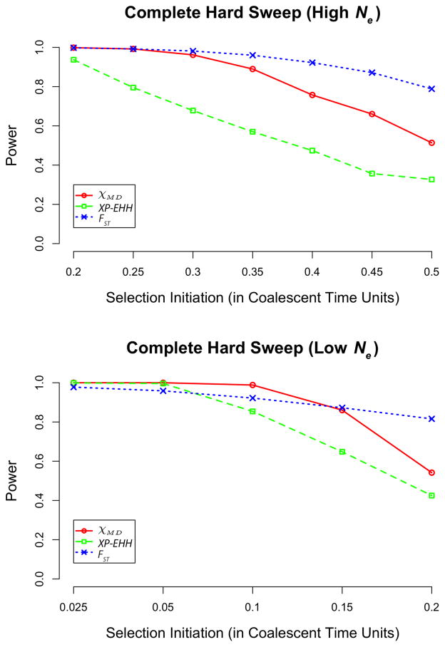
Previous simulation analysis of single-population summary statistics for detecting selective sweeps has pointed to a fairly brief window for their detection. For example, by 0.15 coalescent units (i.e. 0.6N_e generations) after a selective sweep, Przeworksi (2002) found that the power of Tajima’s (1989) D had been reduced to around 30%, while the rejection rate of Fay and Wu’s (2000) H was close to the false positive rate. As expected, our analysis of population-specific classic sweeps also showed that power for each statistic decreased as selection initiation was pushed further back (Figure 1; Table S5). However, the temporal signal of selection was notably extended for these population comparison statistics. F_ST showed the strongest performance, with an exceptionally long-lasting signal of selection. Thus, even in the absence of ongoing selection against migrant alleles, sweeps that differentiate fairly anciently-isolated populations may still be detectable. χ_MD, which excludes singleton polymorphisms to avoid loss of power due to new mutations, outperformed XP-EHH for older hard sweeps. χ_MD still retained roughly 50% power at 0.2 coalescent units after a sweep in the low N_e, s = 0.01 case, and maintained this performance until 0.5 coalescent units after the high N_e, s = 0.001 sweep scenario.

Figure 1.

Power of each statistic for complete hard sweeps for high N_e (top) and low N_e cases (bottom). Note the difference in selection initiation times of the x axes.

Partial hard sweeps

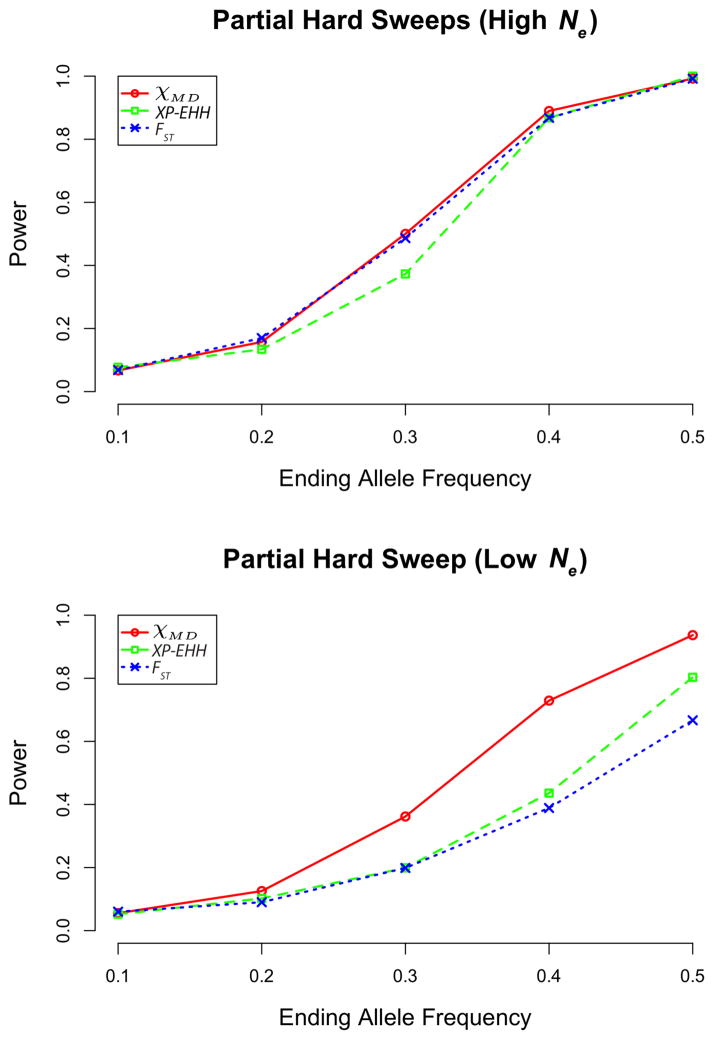
Statistical power from partial hard sweep simulations (Figure 2; Table S5) showed an intuitive increase from a final adaptive allele frequency of 10% (for which power was minimal) to 50% (for which all statistics had strong power). χ_MD displayed superior power for the low N_e case. The statistics had generally similar performance for high N_e partial sweeps, with χ_MD and F_ST ahead of XP-EHH in some instances.

Figure 2.

Power of each statistic tested for partial hard sweeps, for high N_e (top) and low N_e cases (bottom).

Complete and partial soft sweeps

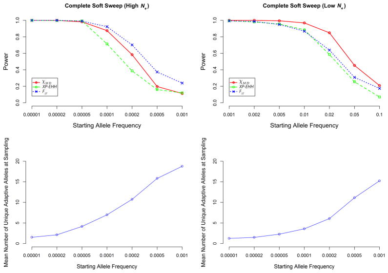
Soft sweeps act on standing variation (as simulated here) or else on recurrent mutations in very large populations. Hence, the adaptive allele may persist on multiple genetic backgrounds within a population after selection, reducing haplotype sharing relative to hard sweeps, and making it more difficult to detect local adaptation. Relatively speaking, softer sweeps are those where the adaptive alleles present at the time of sampling trace back to a larger number of unique chromosomes at the onset of selection. Concordant with previous findings (Pennings and Hermisson 2006), we observed that sweeps become more difficult to detect with increasing softness (Figure 3). In cases where statistical power was neither uniformly high nor uniformly low, χ_MD generally outperformed XP-EHH. For the low N_e case, χ_MD also outperformed F_ST, while in the high N_e case F_ST had an advantage for softer sweeps. Notably, χ_MD was able still to detect a signal of selection in more than 20% of the low N_e replicates when the starting beneficial allele frequency was as high as 10%.

Figure 3.

For complete soft sweeps, the top two panels depict power of each tested statistic. The bottom two panels depict the number of unique adaptations of derived allele at the time of sampling to help distinguish the softness of the sweep (where a value close to 1 indicates mostly hard sweeps). Note the change in scale of x axes between the two N_e cases simulated (left and right).

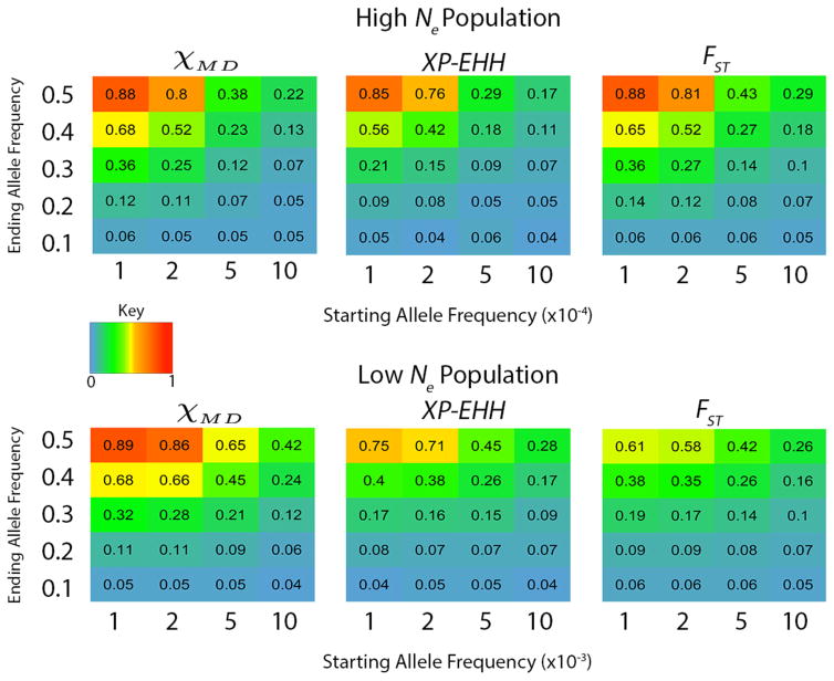
Naturally, incomplete soft sweeps were found to be even more challenging to detect than complete soft sweeps, especially with high initial frequencies and/or low final frequencies of the favored allele (Figure 4). The χ_MD statistic performed particularly impressively in the low N_e simulations, often outperforming XP-EHH and F_ST by significant margins. For high N_e data, performance of the three statistics was more similar, with χ_MD and F_ST often slightly exceeding the power of XP-EHH.

Figure 4.

Heat map depicting power for each statistic for partial soft sweeps. The key refers to powers ranging from 0 to 1. The x axis represents the number of copies of the beneficial allele in the population when the populations split. Note the change in x axes between the two N_e cases (starting frequency per 10,000 or per 1,000). The y axis represent the ending allele frequency at sampling.

Hard and soft sweeps in bottlenecked populations

Until now, we have considered cases of positive selection in populations of constant size. However, we also evaluated a series of population bottleneck scenarios affecting the same population subject to a complete hard or soft sweep (models of particular interest with regard to domestication and the colonization of new environments). In general, bottlenecks are known to reduce genetic variation and to increase the stochastic variance among loci. This increased homozygosity (and, therefore, increased haplotype sharing) in the neutral simulations created higher threshold levels, lowering the power of the tested statistics.

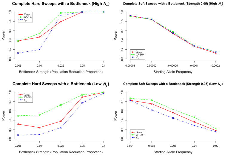
Although bottlenecks presented a challenge for all statistics, XP-EHH often showed the highest power, especially for the low N_e simulations (Figure 5; Table S5). Here, the focus of XP-EHH on a specific haplotype configuration (as opposed to all haplotype identity) may have helped preserve more discriminatory power. F_ST typically performed worse than either haplotype statistic in the presence of bottlenecks, in agreement with the notion that linkage information may be generally helpful in differentiating non-equilibrium demography from positive selection (Jensen et al. 2007).

Figure 5.

Depicted here are power for scenarios with bottlenecks simulated. The left panels depict hard sweeps, with varying strengths of bottlenecks indicated on the x axis. The right panels depict a single bottleneck strength (0.05) with varying starting allele frequencies. Additional cases are summarized in Table S5.

Detecting local selection in the presence of migration

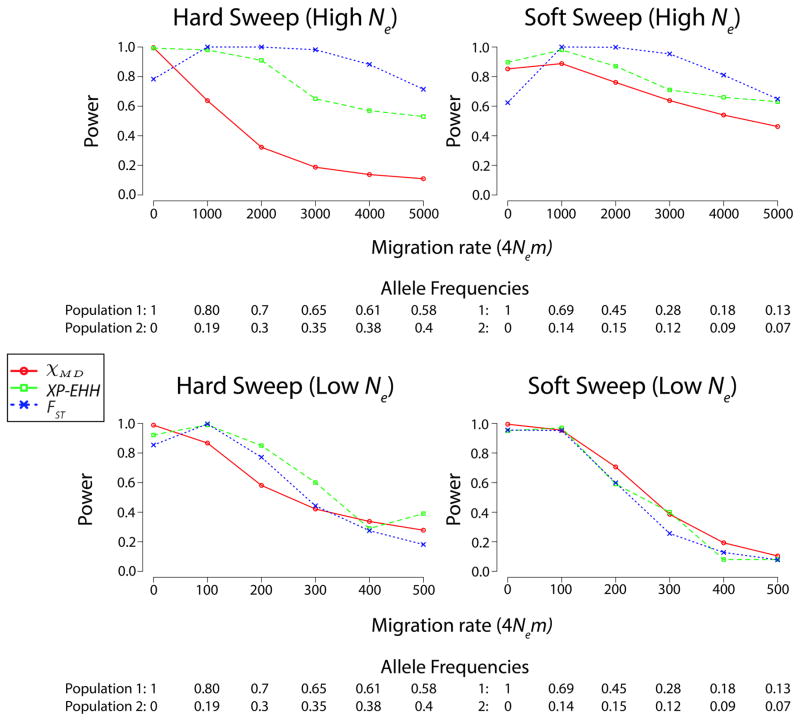
We also investigated scenarios in which migration occurred between diverged populations (Table S5), under a standard isolation-migration model. Results from very high migrations rates are presented here, because the power of each statistic was mostly unaffected until migration rates were increased enough to keep F_ST close to 0 under neutrality. Figure 6 illustrates statistical performance in cases of very high migration rates that typically prevent the beneficial allele from becoming a fixed difference. Particularly for F_ST, selection scenarios with lower migration rates were often easier to detect than those with no migration, suggesting that ongoing selection against migrant alleles may have increased power (note that the onset of selection in some scenarios was fairly ancient; Materials and Methods). For the low N_e cases, all three statistics showed similar performance in the presence of migration. For the high N_e scenarios, F_ST gave the highest power, potentially due to ongoing differentiation at the target site and very closely linked variants (leading to modest window F_ST values that still exceeded the even smaller values under neutrality). XP-EHH also shows an advantage over χ_MD, particularly for the ancient hard sweep case examined. Here, the association between long haplotypes and a specific allele at the target site may preserve a signal for XP-EHH, even if overall levels of haplotype sharing become relatively similar between the two populations.

Figure 6.

Migration was simulated for a subset of scenarios. The high levels of migration that affected statistical performance were sufficient to prevent fixed differences at the target site. Allele frequencies at sampling for both populations are shown below each migration rate.

Effects of allele frequency threshold and sample size

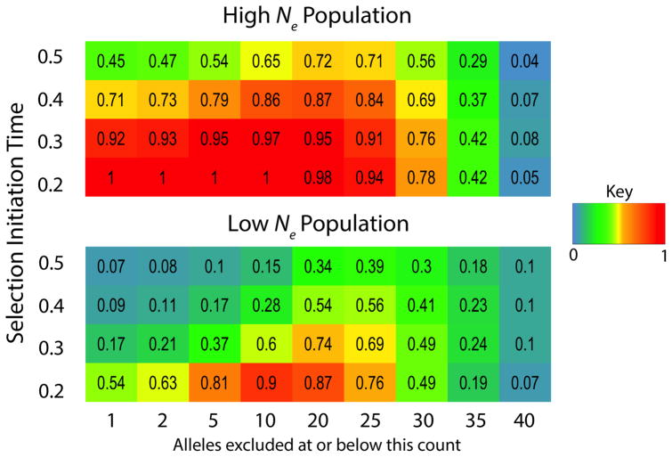
We found that the power to detect old sweeps, already notable for these statistics relative to single population approaches, could be substantially improved for χ_MD by increasing our allele frequency threshold to exclude more than just singletons (Figure 7). This result is intuitive because as time passes after a sweep, new mutations start drifting to higher frequencies, and non-singleton SNPs disrupt otherwise identical haplotypes that had been homogenized by the sweep. Frequency thresholds as high as 20 or 25 percent (out of the combined two population sample size of 100) were favored for sweeps as ancient as 0.4 or 0.5 coalescent units. These results suggest that a localized absence of intermediate frequency alleles may carry a previously unappreciated signal of ancient positive selection.

Figure 7.

This heat map depicts power of the χ_MD statistic as a function of allele frequency threshold (minimum frequency of allele to be included in analysis) and the time (in coalescent units) since the initiation of a complete hard selective sweep. The exclusion of all but intermediate frequency alleles yields surprising power to detect very ancient sweeps.

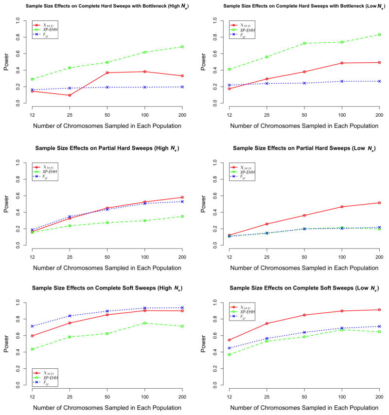
As would be predicted, power for each statistic increased with increasing sample size (Figure 8; Table S5). In general, the sample size of 50 chromosomes per population used in the preceding analyses appears to represent a good compromise between sequencing effort and power. Additional power was observed with larger samples, but with some diminishing returns.

Figure 8.

Sample size effects on each statistic. Bottleneck strength in the high N_e case is 0.01 while in the low N_e case it is 0.025. Ending frequency of partial hard sweeps is 0.3. Starting allele frequency is 0.001 for the high N_e complete soft sweep is and 0.02 for the low N_e case.

Impact of window length and threshold proportion

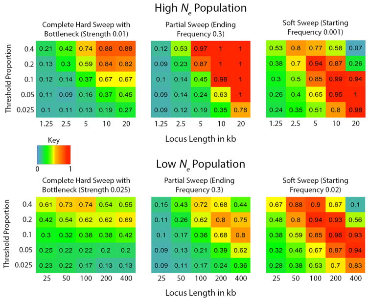
Simulated window lengths and threshold proportions were investigated for the χ_MD statistic (Figure 9; Table S5). Here, threshold proportion refers to the fraction of the window that must be identical between a pair of haplotypes to count toward the total. Diagonal “ridges” of high power are sometimes observed in Figure 8, suggesting an optimum threshold length (i.e. window length × threshold proportion) for a given selection scenario. However, this optimum depends not only on the species, but also on the nature of selection (e.g. hard vs. soft sweeps), suggesting that no single configuration is universally advantageous. It should be noted that the scenarios simulated in this study involved relatively strong selection (s = 0.001 and s = 0.01), so that sweeps would finish within a proscribed time frame. If selection is typically weaker in the species of interest, the shorter shared haplotypes that result could favor a smaller threshold length than indicated by Figure 9 (see Discussion).

Figure 9.

For selected sweep scenarios, this heat map shows χ_MD power for differing window lengths and threshold proportions (the fraction of a window that must be identical between two haplotypes).

Sliding window analyses

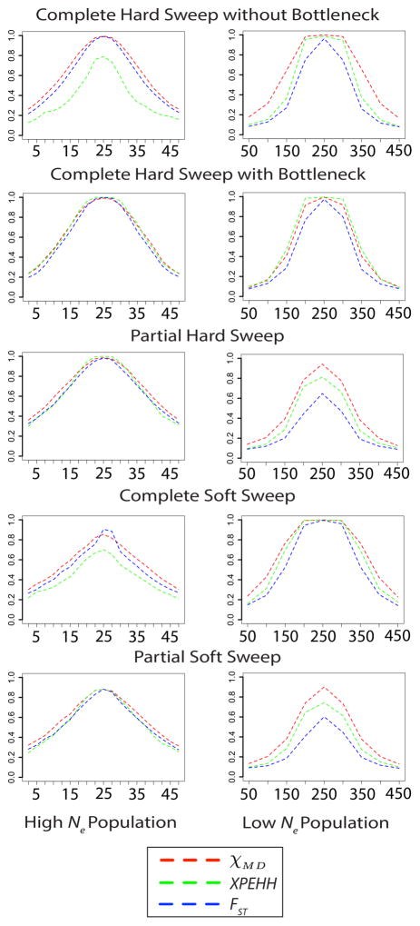
All three statistics were evaluated in sliding windows along a locus so that the effects of physical distance from the selected site could be observed. Intuitively, powers for all three statistics decreased with distance from the site of selection (Figure 10; Table S5). Minor differences were observed in the spatial extent of the three statistics’ signals. The two haplotype signals often displayed wider signals than F_ST, and χ_MD sometimes showed a slightly broader signal than XP-EHH.

Figure 10.

For a subset of sweep scenarios, this figure illustrates the decay of all three statistics’ power by distance (kilobases on the x axis). In the non-bottleneck complete hard sweep, the high N_e populations split at 0.5 time units in the past and selection (s = 0.001) began at 0.2 time units in the past. In the low N_e population, the populations split at 0.2 time units in the past and selection (s = 0.01) began immediately. The bottleneck strength in the high N_e case is 0.05 and the low N_e case is 0.1. In both cases of the partial hard sweep, the ending allele frequencies were 0.5. In the complete soft sweep cases for both populations, starting frequency was 0.001. In the partial soft sweep cases for the high N_e case, starting allele frequency was 0.0001 and ending allele frequency was 0.5. For the high N_e case, beneficial starting allele frequency was 0.001 and ended at 0.5.

Comparison with single population statistics

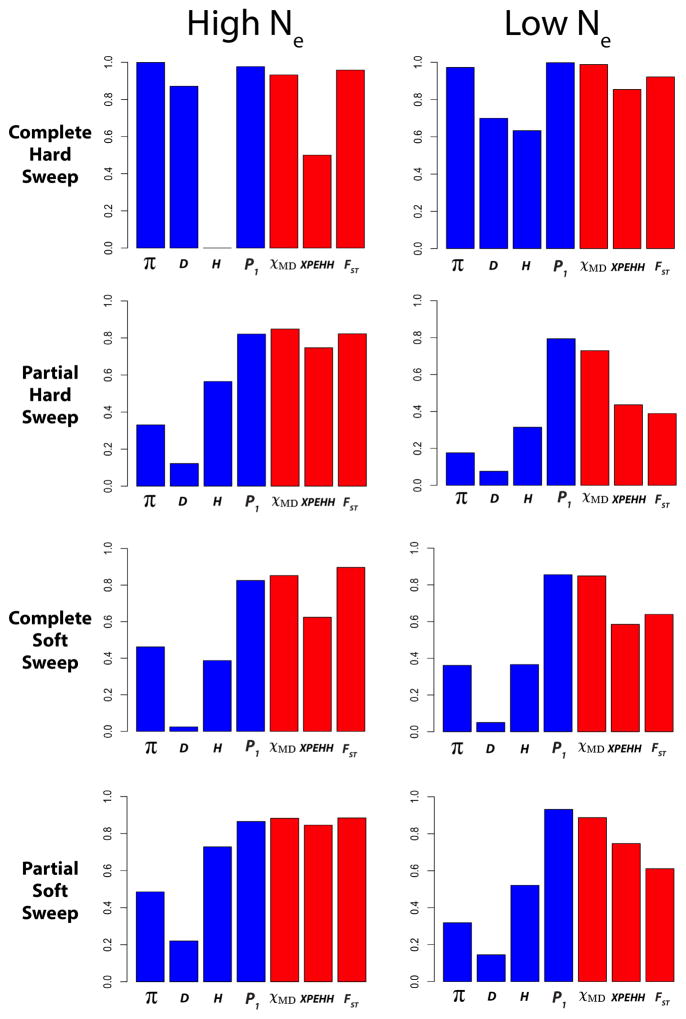
In general, single population statistics were outperformed by cross-population statistics (Figure 11; Table S5), underscoring the advantage of controlling for shared history in the ancestral population. An exception was power for the haplotype statistic P₁, which was essentially unaffected by the use of only one population. Thus, under the conditions simulated, the P₁ statistic (quantifying the haplotype sharing of population 1) is quite sensitive a wide range of selective sweep scenarios. However, adding a second population may add important robustness to empirical studies. In these simulations, a specific known recombination rate was used. Using a second population helps control for the historical recombination rate, which would not necessarily be known in a real data set, making it difficult to predict how a single population haplotype statistic should behave under neutrality. Further, the use of a second population can also control for demographic and selective events in the ancestral population, which were not simulated in this study.

Figure 11.

The power of four single population statistics was calculated for an older complete hard sweep, a partial hard sweep, a complete soft sweep, and a partial soft sweep. Note that simulation parameters differ between the high N_e and low N_e cases (Materials and Methods).

Nucleotide diversity (π), Tajima’s D, and Fay and Wu’s H had varying power in each sweep scenario. Fay and Wu’s H, for instance, showed moderately high power in partial and/or soft sweep scenarios, but low power in the complete hard sweep scenarios (particularly in the large N_e case, where the longer time since selection erases the signal of high frequency derived alleles; Przeworski 2002). In contrast, the between-population statistics showed relatively high power in each sweep scenario, a critical advantage since we do not know which kind of selection to expect in a real data set.

Empirical analysis of Drosophila genomes

To examine the performance of cross-population statistics on empirical data, we analyzed fully sequenced D. melanogaster genomes from the Drosophila Genome Nexus (Lack et al. 2015). Specifically, we compared variation between the Rwanda-Gikongoro population sample (27 genomes) and the Zambia-Siavonga population sample (197 genomes). Being sequenced to averaged depths of >27X (Lack et al. 2015) from haploid female gametes (Langley et al. 2011), these genomes have the advantage of clearly defined haplotypes.

Zambia appears to represent an ancestral range population, while Rwanda and other equatorial African populations may reflect range expansion (Pool et al. 2012). The range of selective pressures that may differ between these populations is unknown, but geographic and climate differences do exist. The Rwanda location features a higher altitude (1930 versus 530 meters above sea level) and greater rainfall, while Zambia has more seasonal variation in temperature and a longer dry season.

Applying χ_MD, XP-EHH (again bounded as a window statistic), and F_ST to this genomic dataset, we were able to study statistic correlations as well as perform a GO enrichment analysis. Each genomic window has a value for χ_MD, XP-EHH, and F_ST (Table S6) and thus, has an associated quantile or empirical P value for each statistic as well. Moderately strong correlations were observed between all three statistics (Table 2; Figure S3), with the highest correlation between XP-EHH and F_ST.

Table 2.

Window quantile correlations are shown among the three between-population statistics evaluated for the Drosophila genomic data set. Conditional probability refers to the probability that a window is within the 5% tail of one statistic, given that it is within the 5% tail of another statistic. Because the number of outliers is the same for each statistic, these probabilities are symmetric.

Statistics	Correlation Coefficient	Conditional Probability
χMD, XP-EHH	0.5395	0.3529
χMD, FST	0.4827	0.4029
XP-EHH, FST	0.5713	0.4837

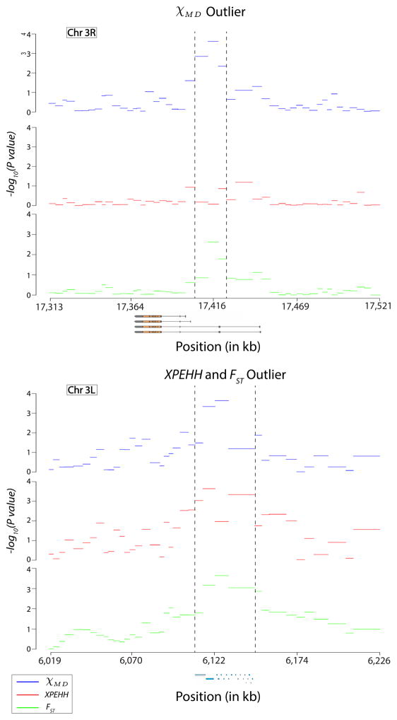
Figure 12 depicts the most extreme outlier regions for each statistic as well as their flanking regions. The χ_MD outlier, located within the Insulin-like receptor gene, was also detected by F_ST but not by XP-EHH. XP-EHH and F_ST identified the same maximal outlier region, amongst a group of cuticle protein genes, which was also flagged by χ_MD.

Figure 12.

The top outlier regions and flanking windows for the empirical analysis of χ_MD, XP-EHH, and F_ST are shown. Above, the χ_MD outlier resides within a transcript region of the insulin receptor gene (InR alternative transcripts are shown). Below, XP-EHH and F_ST reached their maxima in the same outlier region (at adjacent windows), within a cluster of cuticle-related genes.

We performed gene ontology enrichment analysis on the results for each statistic (Materials and Methods). Our primary goal for this exploratory analysis was to investigate the degree to which different statistics find evidence for selection in the same functional categories of genes. We found fairly strong overlap between the biological processes implicated by χ_MD, XP-EHH, and F_ST (Figure S4). Complete results are given in Table S7, while a set of the most enriched terms for each statistic is given in Table 3. While each statistic implicated a unique combination of GO categories, all lists included functions related to sensory perception and apoptosis. Differences in the genes and categories detected by each statistic may reflect both false positives and differences in the type and timing of selection impacting different genes and functional categories.

Table 3.

Selected biological processes enriched for outliers of each statistic are given. For each statistic, biological process GO categories represented in at least five outlier regions were identified. Of those with raw permutation P value below 0.01, the categories with the highest proportion of outliers are listed here. Highly similar GO categories were omitted to minimize redundancy.

		Windows	χMD	χMD	XP-EHH	XP-EHH	FST	FST
GO ID	Description	w/ Genes	Outliers	P	Outliers	P	Outliers	P
χMD Enrichment
43524	negative regulation of neuron apoptotis	13	7	0.001	4	0.103	4	0.054
32006	regulation of TOR signaling cascade	11	5	0.008	5	0.006	3	0.095
48190	wing disc dorsal/ventral pattern formation	46	16	0.004	13	0.031	9	0.159
9582	detection of abiotic stimulus	55	18	0.002	17	0.002	13	0.016
45448	mitotic cell cycle, embryonic	28	9	0.004	1	0.977	6	0.050
7602	phototransduction	43	13	0.007	13	0.004	11	0.007
31124	mRNA 3'-end processing	30	9	0.002	5	0.201	3	0.551
6289	nucleotide-excision repair	24	7	0.003	6	0.013	4	0.102
6401	RNA catabolic process	32	8	0.009	7	0.026	3	0.507
22613	ribonucleoprotein complex biogenesis	35	8	0.006	7	0.021	7	0.011
42451	purine nucleoside biosynthetic process	44	10	0.007	6	0.209	10	0.002
6260	DNA replication	66	14	0.004	7	0.466	13	0.002
70647	prot. modif. by small prot. conjug./removal	91	19	0.002	17	0.009	16	0.004
8340	determination of adult lifespan	145	30	0.001	19	0.261	26	0.001
6310	DNA recombination	56	11	0.006	9	0.039	8	0.049
XP-EHH Enrichment
32006	regulation of TOR signaling cascade	11	5	0.008	5	0.006	3	0.095
6917	induction of apoptosis	20	5	0.251	8	0.007	6	0.029
71453	cellular response to oxygen levels	28	7	0.130	10	0.003	7	0.044
6816	calcium ion transport	31	9	0.050	11	0.003	10	0.002
7369	gastrulation	31	8	0.133	11	0.004	10	0.003
46662	regulation of oviposition	18	1	0.909	6	0.009	3	0.238
9581	detection of external stimulus	60	19	0.002	19	0.001	15	0.005
10942	positive regulation of cell death	53	9	0.619	16	0.006	13	0.013
8344	adult locomotory behavior	60	16	0.018	16	0.010	11	0.098
7291	sperm individualization	45	9	0.047	11	0.005	10	0.004
52548	regulation of endopeptidase activity	47	9	0.051	11	0.005	10	0.004
50906	detect. stimulus involved in sensory percept.	84	14	0.167	19	0.003	19	<0.001
9416	response to light stimulus	119	25	0.014	26	0.003	25	<0.001
7349	cellularization	94	16	0.064	20	0.002	18	0.002
43900	regulation of multi-organism process	81	9	0.689	17	0.009	17	0.001
FST Enrichment
35072	ecdysone-mediated induction of salivary gland cell autophagic cell death	11	3	0.622	5	0.083	6	0.005
7157	heterophilic cell-cell adhesion	25	10	0.098	11	0.019	13	<0.001
61057	peptidoglycan recog. prot. signal. pathway	10	2	0.228	3	0.052	5	<0.001
35073	pupariation	11	2	0.386	1	0.740	5	0.002
51260	protein homooligomerization	17	6	0.034	5	0.090	7	0.002
35303	regulation of dephosphorylation	13	4	0.033	4	0.029	5	0.002
6963	pos. regul. of antibact. peptide biosynthesis	21	3	0.612	3	0.565	8	0.001
43279	response to alkaloid	22	2	0.859	5	0.165	8	0.002
12502	induction of programmed cell death	31	7	0.318	11	0.006	11	0.001
43523	regulation of neuron apoptotic process	17	8	0.001	5	0.064	6	0.007
10950	pos. regulation of endopeptidase activity	17	5	0.045	5	0.039	6	0.004
45088	regulation of innate immune response	20	3	0.468	2	0.712	7	0.002
71897	DNA biosynthetic process	27	6	0.036	5	0.099	9	<0.001
50911	detection of chemical stimulus involved in sensory perception of smell	40	5	0.552	10	0.011	13	<0.001
16337	cell-cell adhesion	80	25	0.083	25	0.028	26	<0.001

DISCUSSION

Detecting cases of local selection is critical for the study of agricultural domestication, conservation, and human biology, as well as our basic understanding of adaptation and its genetic basis. However, positive selection can have different forms at the population genetic level (hard vs. soft sweeps, complete vs. partial sweeps), and may or may not have occurred very recently in population genetic time. Especially when data from only one population is available, it can be very difficult to find statistical methods able to detect such a wide variety of adaptive scenarios. Here, we show that detecting diverse modes of positive selection is often possible when comparing genetic variation from two populations with adaptive differences.

We have introduced a statistic, χ_MD, that compares the total pairwise haplotype identity within each of two populations, and compared its performance against another haplotype statistic (XP-EHH) and an index of allele frequency differentiation (F_ST). F_ST often had fairly similar power to detect local selection as the haplotype statistics. Although joint approaches are not a focus of the present study, it may be advantageous in many scenarios to use F_ST and a haplotype metric as complementary statistics. Relative to the haplotype approaches, F_ST often had stronger performance for older (hard) sweeps and weaker power for population bottleneck scenarios with hard or soft sweeps.

Focusing on the differences between the χ_MD and XP-EHH haplotype statistics, the primary performance advantage observed for XP-EHH was for selection in bottlenecked populations. XP-EHH had important advantages for certain bottleneck and migration scenarios. Hence, the specific haplotype configuration sought by the EHH approach appears to confer some robustness against demographic sources of haplotype identity.

Notably, however, χ_MD showed superior power to XP-EHH in most other scenarios. For hard sweeps, the statistical signal of χ_MD is more enduring than for XP-EHH. The longer-lasting signal of χ_MD may stem partly from the masking of rare variation, which prevents post-selection mutations from interrupting haplotype identity. χ_MD may also be more tolerant of recombination during or after selection, since identical haplotype blocks do not need to maintain their original linkage configuration in order to contribute to summed haplotype identity.

In addition, χ_MD displayed greater power than XP-EHH for many cases of partial and/or soft sweeps. For the low N_e partial and soft sweep cases, χ_MD showed performance advantages over both XP-EHH and F_ST. These results underscore the versatility of χ_MD for detecting population-specific selection. This flexibility reflects a very basic signal of directional selection that χ_MD responds to: haplotype sharing between alleles with unusually recent common ancestry. This signal is produced even if multiple haplotypes carry the beneficial mutation, or if this mutation has not reached high frequency.

Being a window-based approach, χ_MD is particularly well-suited to analyzing fully sequenced genomes. Though implemented in kilobase-defined windows in this simulation study, in real genomes it may be preferable to apply χ_MD in windows scaled by genetic distance or by numbers of variable sites (as implemented in the Drosophila case studied here). The window orientation of χ_MD also makes it dramatically more computationally efficient than XP-EHH, which must be evaluated separately for every variable site that passes filtering criteria. This difference also implies that many fewer tests need to be performed for a genome-wide analysis of χ_MD in comparison to XP-EHH, although we have shown that XP-EHH still maintains significant power when applied in a window-maximum format.

When applying χ_MD to empirical data, two general issues should be carefully considered. One is the parameterization of χ_MD in terms of window and threshold length, and allele frequency threshold. Although we offer preliminary guidance through the simulation analyses shown here, we recommend that potential users conduct similar simulations reflecting the genetic properties and demographic histories of their own study populations, along with selective sweep models of potential interest (in terms of strength, hardness, and timing), in order to fine-tune χ_MD settings.

A second major issue, relevant to any population genomic analysis, is the determination of statistical significance. If demographic parameter estimates are available that are reliable, or at least conservative with respect to intrapopulation shared haplotype lengths, then neutral simulations can be performed to obtain the probability of observing a given χ_MD value without selection. If researchers need to establish whether a given value is unexpected genome-wide, then clearly a multiple testing correction is also needed (e.g. Storey and Tibshirani 2003). If no credible demographic model is available, then the user is most likely restricted to an outlier framework to identify preliminary candidates for local adaptation.

Throughout this analysis, we have assumed that the phase of each haplotype is known with certainty. In some organisms, including Drosophila, it is possible to sequence completely or mostly homozygous genomes (e.g. Langley et al. 2011; Mackay et al. 2012). But for many diploid non-laboratory organisms, including humans, it is not yet practical to empirically obtain genome-wide phasing data unless family groups (e.g. parent-child trios) are sequenced. Although haplotype phasing can be estimated computationally (e.g. Scheet and Stephens 2006), the bias entailed by such methods for haplotype statistics like χ_MD is unclear. Alternatively, an unphased counterpart to χ_MD could be envisioned in which homozygosity runs shared between individuals are totaled.

The simple χ_MD statistic appears to be quite useful in its current form, but future advances over the present approach are certainly conceivable. The probability of a specific shared haplotype length under the null hypothesis could be evaluated via theory (Harris and Nielsen 2013) or simulation, potentially eliminating the need for a threshold length. Information could also be combined across windows to delineate the boundaries of non-neutral regions, or window size could be adjusted based on observed genetic variation (Pavlidis et al. 2010). Lastly, the signal of haplotype identity could be combined with information from the two-population allele frequency spectrum and other aspects of genetic variation. Still, the present work represents a “proof of concept” that haplotype identity tracts efficiently capture the signal of diverse modes of positive selection, often performing as well or better than published statistics at distinguishing neutral from non-neutral histories.

Supplementary Material

Supp Fig S1-S4

Figure S1. Depicted here are distributions of all three statistics for various scenarios of high N_e scenarios. In the non-bottleneck hard sweep case, the populations split at 0.5 coalescent time units in the past and selection began at 0.2 time unites in the past. In the bottleneck scenario, the bottleneck strength was 0.05. The ending frequency of the partial hard sweep is 0.5. The starting frequency of the complete soft sweep was 0.001. The starting allele frequency was 0.0001 and ended at 0.5 for the partial soft sweep case.

Figure S2. Depicted here are distributions of all three statistics for various scenarios of low N_e scenarios. In the non-bottleneck hard sweep case, the populations split at 0.2 coalescent time units in the past and selection began immediately. In the bottleneck scenario, the bottleneck strength was 0.1. The ending frequency of the partial hard sweep is 0.5. The starting frequency of the complete soft sweep was 0.001. The starting allele frequency was 0.001 and ended at 0.5 for the partial soft sweep case.

Figure S3. Based on evaluating the three between-population statistics in published Drosophila genomes, this figure shows the correlation between their empirical P values across all autosomal windows. Each cell represents the number of autosomal genomic windows whose statistic P values are within the corresponding range of the cell.

Figure S4. The gene ontology categories identified by each statistic show substantial overlap. This analysis focuses on the 1,988 biological process GO categories represented in at least ten different genomic windows. Part A depicts the number of such categories with a raw permutation P value below 0.05 for each statistic. Part B includes the lowest 200 P values for each statistic.

LITERATURE CITED

- Bonin A, Nicole F, Pompanon F, Miaud C, Taberlet P. Population Adaptive Index: a new method to help measure intraspecific genetic diversity and prioritize populations for conservation. Cons Biol. 2007;21:697–708. doi: 10.1111/j.1523-1739.2007.00685.x. [DOI] [PubMed] [Google Scholar]
- Comeron JM, Ratnappan R, Bailin A. The many landscapes of recombination in Drosophila melanogaster. PLoS Genetics. 2012;8:e1002905. doi: 10.1371/journal.pgen.1002905. [DOI] [PMC free article] [PubMed] [Google Scholar]
- Ewing G, Hermisson J. MSMS: a coalescent simulation program including recombination, demographic structure and selection at a single locus. Bioinformatics. 2010;26:2064–2065. doi: 10.1093/bioinformatics/btq322. [DOI] [PMC free article] [PubMed] [Google Scholar]
- Fariello MI, Boitard S, Naya H, SanCristobal M, Servin B. Detecting signatures of selection through haplotype differentiation among hierarchically structured populations. Genetics. 2013;193:929–941. doi: 10.1534/genetics.112.147231. [DOI] [PMC free article] [PubMed] [Google Scholar]
- Fay JC, Wu CI. Hitchhiking under positive Darwinian selection. Genetics. 2000;155:1405–1413. doi: 10.1093/genetics/155.3.1405. [DOI] [PMC free article] [PubMed] [Google Scholar]
- Ferrer-Admetlla A, Liang M, Korneliussen T, Nielsen R. On detecting incomplete soft or hard selective sweeps using haplotype structure. Mol Biol Evol. 2014;31:1275–1291. doi: 10.1093/molbev/msu077. [DOI] [PMC free article] [PubMed] [Google Scholar]
- Fumagalli M, Sironi M, Pozzoli U, Ferrer-Admettla A, Pattini L, et al. Signatures of environmental genetic adaptation pinpoint pathogens as the main selective pressure through human evolution. PLoS Genet. 2011;7:e1002355. doi: 10.1371/journal.pgen.1002355. [DOI] [PMC free article] [PubMed] [Google Scholar]
- Hancock AM, Witonsky DB, Alkorta-Aranburu G, Beall CM, Gebremedhin A, et al. Adaptations to climate-mediated selective pressures in humans. PLoS Genet. 2011;7:e1001375. doi: 10.1371/journal.pgen.1001375. [DOI] [PMC free article] [PubMed] [Google Scholar]
- Harris K, Nielsen R. Inferring demographic history from a spectrum of shared haplotype lengths. PLoS Genet. 2013;9:e1003521. doi: 10.1371/journal.pgen.1003521. [DOI] [PMC free article] [PubMed] [Google Scholar]
- Hudson RR. Generating samples under a Wright-Fisher neutral model of genetic variation. Bioinformatics. 2002;18:337–338. doi: 10.1093/bioinformatics/18.2.337. [DOI] [PubMed] [Google Scholar]
- Hudson RR, Slatkin M, Maddison WP. Estimation of levels of gene flow from DNA sequence data. Genetics. 1992;132:583–589. doi: 10.1093/genetics/132.2.583. [DOI] [PMC free article] [PubMed] [Google Scholar]
- Jensen JD, Thornton KR, Bustamante CD, Aquadro CF. On the utility of linkage disequilibrium as a statistic for identifying targets of positive selection in nonequilibrium populations. Genetics. 2007;176:2371–2379. doi: 10.1534/genetics.106.069450. [DOI] [PMC free article] [PubMed] [Google Scholar]
- Lack JB, Cardeno CM, Crepeau MW, Taylor W, Corbett-Detig RB, Stevens KA, Langley CH, Pool JE. The Drosophila Genome Nexus: a population genomic resource of 623 Drosophila melanogaster genomes, including 197 from a single ancestral range population. Genetics. 2015;199:1229–1241. doi: 10.1534/genetics.115.174664. [DOI] [PMC free article] [PubMed] [Google Scholar]
- Langley CH, Crepeau M, Cardeno C, Corbett-Detig R, Stevens K. Circumventing heterozygosity: sequencing the amplified genome of a single haploid Drosophila melanogaster embryo. Genetics. 2011;188:239–246. doi: 10.1534/genetics.111.127530. [DOI] [PMC free article] [PubMed] [Google Scholar]
- Mackay TFC, Richards S, Stone EA, Barbadilla A, Ayroles J, et al. The Drosophila melanogaster genetic reference panel. Nature. 2012;482:173–178. doi: 10.1038/nature10811. [DOI] [PMC free article] [PubMed] [Google Scholar]
- Micallef L, Rodgers P. eulerAPE: Drawing area-proportional 3-Venn diagrams using ellipses. PLoS ONE. 2014;9:e101717. doi: 10.1371/journal.pone.0101717. [DOI] [PMC free article] [PubMed] [Google Scholar]
- Pavlidis P, Jensen JD, Stephan W. Searching for footprints of positive selection in whole-genome SNP data from nonequilibrium populations. Genetics. 2010;185:907–922. doi: 10.1534/genetics.110.116459. [DOI] [PMC free article] [PubMed] [Google Scholar]
- Pennings PS, Hermisson J. Soft sweeps III: the signature of positive selection from recurrent mutation. PLoS Genet. 2006;2:e186. doi: 10.1371/journal.pgen.0020186. [DOI] [PMC free article] [PubMed] [Google Scholar]
- Pickrell JK, Coop G, Novembre J, Kudaravalli S, Li J, et al. Signals of recent positive selection in a worldwide sample of human populations. Genome Res. 2009;19:826–837. doi: 10.1101/gr.087577.108. [DOI] [PMC free article] [PubMed] [Google Scholar]
- Pool JE, Aquadro CF. The genetic basis of adaptive pigmentation variation in Drosophila melanogaster. Mol Ecol. 2007;16:2844–2851. doi: 10.1111/j.1365-294X.2007.03324.x. [DOI] [PMC free article] [PubMed] [Google Scholar]
- Pool JE, Corbett-Detig RB, Sugino RP, Stevens KA, Cardeno CM, Crepeau MW, Duchen P, Emerson JJ, Saelao P, Begun DJ, Langley CH. Population genomics of sub-Saharan Drosophila melanogaster: African diversity and non-African admixture. PLoS Genetics. 2012;8:e1003080. doi: 10.1371/journal.pgen.1003080. [DOI] [PMC free article] [PubMed] [Google Scholar]
- Przeworski M. The signature of positive selection at randomly chosen loci. Genetics. 2002;160:1179–1189. doi: 10.1093/genetics/160.3.1179. [DOI] [PMC free article] [PubMed] [Google Scholar]
- Rebeiz M, Pool JE, Kassner VA, Aquadro CF, Carroll SB. Stepwise modification of a modular enhancer underlies adaptation in a Drosophila population. Science. 2009;326:1663–1667. doi: 10.1126/science.1178357. [DOI] [PMC free article] [PubMed] [Google Scholar]
- Roesti M, Gavrilets S, Hendry AP, Salzburger W, Berner D. The genomic signature of parallel adaptation from shared genetic variation. Mol Ecol. 2014;23:3944–3956. doi: 10.1111/mec.12720. [DOI] [PMC free article] [PubMed] [Google Scholar]
- Sabeti PC, Reich DE, Higgins JM, Levine HZP, Richter DJ, et al. Detecting recent positive selection in the human genome from haplotype structure. Nature. 2002;419:832–837. doi: 10.1038/nature01140. [DOI] [PubMed] [Google Scholar]
- Sabeti PC, Varilly P, Fry B, Lohmueller J, Hostetter E, et al. Genome-wide detection and characterization of positive selection in human populations. Nature. 2007;449:913–918. doi: 10.1038/nature06250. [DOI] [PMC free article] [PubMed] [Google Scholar]
- Santiago E, Caballero A. Variation after a selective sweep in a subdivided population. Genetics. 2005;169:475–483. doi: 10.1534/genetics.104.032813. [DOI] [PMC free article] [PubMed] [Google Scholar]
- Scheet P, Stephens M. A fast and flexible statistical model for large-scale population genotype data: applications to inferring missing genotypes and haplotypic phase. Am J Hum Genet. 2006;78:629–644. doi: 10.1086/502802. [DOI] [PMC free article] [PubMed] [Google Scholar]
- Schlötterer C, Dieringer D. A novel test statistic for the identification of local selective sweeps based on microsatellite gene diversity. In: Nurminsky D, editor. Selective Sweep. Molecular Biology Intelligence Unit; 2005. pp. 55–64. [Google Scholar]
- Schrider DR, Houle D, Lynch M, Hahn MW. Rates and genomic consequences of spontaneous mutational events in Drosophila melanogaster. Genetics. 2013;194:937–954. doi: 10.1534/genetics.113.151670. [DOI] [PMC free article] [PubMed] [Google Scholar]
- Storey JD, Tibshirani R. Statistical significance for genomewide studies. Proceedings of the National Academy of Sciences. 2003;100:9440–9445. doi: 10.1073/pnas.1530509100. [DOI] [PMC free article] [PubMed] [Google Scholar]
- Storz JF, Kelly JK. Effects of spatially varying selection on nucleotide diversity and linkage disequilibrium: insights from deer mouse globin genes. Genetics. 2008;180:367–379. doi: 10.1534/genetics.108.088732. [DOI] [PMC free article] [PubMed] [Google Scholar]
- Tajima F. Statistical method for testing the neutral mutation hypothesis by DNA polymorphism. Genetics. 1989;123:585–595. doi: 10.1093/genetics/123.3.585. [DOI] [PMC free article] [PubMed] [Google Scholar]
- Voight BF, Kudaravalli S, Wen X, Pritchard JK. A map of recent positive selection in the human genome. PLoS Biol. 2006;4:e72. doi: 10.1371/journal.pbio.0040072. [DOI] [PMC free article] [PubMed] [Google Scholar]
- Will JL, Kim HS, Clarke J, Painter JC, Fay JC, et al. Incipient balancing selection through adaptive loss of aquaporins in natural Saccharomyces cerevisiae populations. PLoS Genetics. 2010;6:e1000893. doi: 10.1371/journal.pgen.1000893. [DOI] [PMC free article] [PubMed] [Google Scholar]
- Wright S. Evolution in Mendelian populations. Genetics. 1931;16:97–159. doi: 10.1093/genetics/16.2.97. [DOI] [PMC free article] [PubMed] [Google Scholar]
- Yi X, Liang Y, Huerta-Sanchez E, Jin X, Cuo ZX, et al. Sequencing of 50 human exomes reveals adaptation to high altitude. Science. 2010;329:75–78. doi: 10.1126/science.1190371. [DOI] [PMC free article] [PubMed] [Google Scholar]
Associated Data
This section collects any data citations, data availability statements, or supplementary materials included in this article.
Supplementary Materials