

Abstract
In developing improved protein variants by site-directed mutagenesis or recombination, there are often competing objectives that must be considered in designing an experiment (selecting mutations or breakpoints): stability vs. novelty, affinity vs. specificity, activity vs. immunogenicity, and so forth. Pareto optimal experimental designs make the best trade-offs between competing objectives. Such designs are not “dominated”; i.e., no other design is better than a Pareto optimal design for one objective without being worse for another objective. Our goal is to produce all the Pareto optimal designs (the Pareto frontier), in order to characterize the trade-offs and suggest designs most worth considering, but to avoid explicitly considering the large number of dominated designs. To do so, we develop a divide-and-conquer algorithm, PEPFR (Protein Engineering Pareto FRontier), that hierarchically subdivides the objective space, employing appropriate dynamic programming or integer programming methods to optimize designs in different regions. This divide-and-conquer approach is efficient in that the number of divisions (and thus calls to the optimizer) is directly proportional to the number of Pareto optimal designs. We demonstrate PEPFR with three protein engineering case studies: site-directed recombination for stability and diversity via dynamic programming, site-directed mutagenesis of interacting proteins for affinity and specificity via integer programming, and site-directed mutagenesis of a therapeutic protein for activity and immunogenicity via integer programming. We show that PEPFR is able to effectively produce all the Pareto optimal designs, discovering many more designs than previous methods. The characterization of the Pareto frontier provides additional insights into the local stability of design choices as well as global trends leading to trade-offs between competing criteria.
Keywords: protein engineering, protein design, experiment planning, multi-objective optimization, site-directed recombination, site-directed mutagenesis, protein interaction specificity, therapeutic proteins
1 Introduction
Protein engineering tasks often have two or more different goals that may be complementary or even competing. For example, in developing chimeric libraries, the resulting hybrids should be similar enough to the evolutionarily-selected wild-type proteins to be stably folded, but different enough to display functional variation [42, 3, 32, 67, 19]. Similarly, in designing interacting proteins, the partners must bind not only strongly but also specifically [45, 16, 27, 31, 2, 66, 11]. Finally, in deimmunizing therapeutic proteins, the variants must maintain bioactivity while being less immunogenic [6, 7, 44, 43]. Since no design can be optimal for all competing goals, trade-offs must be made. Pareto optimal (undominated) experimental designs are the best representatives for consideration, as each does as well as possible with respect to one goal without further sacrificing the other(s). This paper presents general methods for performing Pareto optimal protein engineering, and demonstrates how to apply them in the scenarios discussed above.
To optimize an experimental design, it is necessary to be able to control some design parameters that specify which variants to produce. Site-directed mutation and site-directed recombination provide the engineer with the ability to precisely specify an experiment, either in terms of specific substitutions for some amino acids (site-directed mutation) or specific positions for crossing over between parents (site-directed recombination). Our approach thus focuses on these two technologies. We treat them separately here, though there is nothing in theory prohibiting optimization of a combined mutation + recombination design. While stochastic methods can be partially controlled (e.g., choosing codons to promote recombination in gene shuffling [17]), we leave for future work the extension of our approach to handle them.
A design (i.e., selected substitutions or breakpoint locations) can be evaluated in silico for its quality with respect to different design objectives that represent the goals of the design task. For example, a mutant can be evaluated for structural perturbation according to ΔΔG° predictors [4, 14, 24] or for structural and functional perturbation according to consistency of the mutations with the evolutionary record [49, 46, 53, 58]. Likewise, a site-directed recombination library can be evaluated for overall perturbation (averaged over the hybrids) according to a sequence-structure potential [60, 42, 48, 47, 65], as well as the sequence diversity of its hybrids [68]. Numerous other criteria exist to evaluate variants (or members of a library) by task-specific sequence and/or structure-based potentials (solubility, crystallizability, level of expression, etc.); one of the examples studied here is immunogenicity as assessed by sequence-based MHC-II epitope predictors [8, 61]. Finally, in designing interacting proteins, potentials have been developed to predict likelihood or strength of interaction (and thereby also specificity) [33, 26, 12, 59, 51, 23].
The design problem can then be summarized as searching over possible sets of values for the design parameters (searching over the design space) to find those that are best according to the design objectives. However, since the design objectives can be complementary and perhaps even competing, we must be more careful in defining best. It is often difficult, and always results in some bias, to decide a priori upon weights for combining objectives; instead it is better to consider specific designs and their relative merits.
Pareto optimization characterizes the designs that make the best trade-offs and are most worth further evaluation and experimental construction. We seek to determine all the Pareto optimal designs—the complete Pareto frontier. Fig. 1 illustrates a design space and its Pareto optimal designs. In the figure, the circled points seem particularly good, since near each one, there is a relatively sharp drop off in one criterion or the other (or both). The optimality of these designs persists over a range of relative weights between the two criteria. If the number of experiments to be conducted is limited, the Pareto optimal designs could be subjected to additional characterization (e.g., applying more expensive modeling techniques or accounting for ease of experimental construction), in order to select the most beneficial. The stability of design choices over the Pareto frontier can also help provide confidence that the designs do not critically depend on small, unreliable differences in the evaluation criteria.
Figure 1.
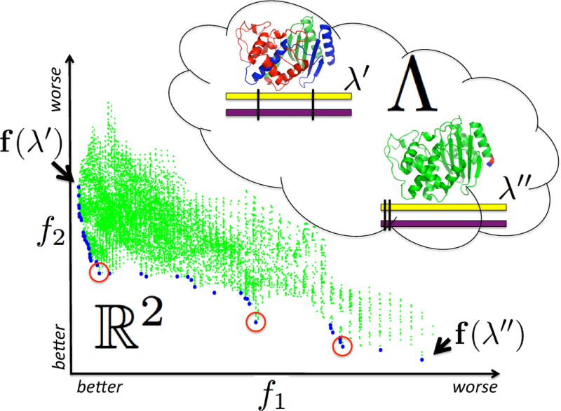
Design of site-directed recombination experiments with two competing design objectives f1 (here the overall library diversity) and f2 (here the average hybrid stability), each of which is expressed as a function to be minimized (a convention employed throughout). The possible breakpoint locations are the design parameters, defining the design space Λ. Two designs, λ′ and λ″, are illustrated, along with their corresponding evaluations, f(λ′) and f(λ″), in the objective space f1 × f2 ⊂ ℝ2. Blue points in the objective space represent Pareto optimal designs, while green points represent designs that are dominated by the Pareto optimal ones. Our goal is to find all the Pareto optimal designs (the Pareto frontier) without explicitly enumerating and evaluating the combinatorially large number of dominated designs. Characterization of the Pareto frontier enables the identification of designs (such as the circled points) that are most promising in terms of the trade-offs.
The design space typically contains a massive number of designs, resulting from the various combinations of choices for the parameters. For example, the simple two-breakpoint design space illustrated in Fig. 1 contains designs. We could enumerate the entire space for this illustration, but with more breakpoints, it would be undesirable or even infeasible to first generate all the designs and then seek to identify the Pareto frontier. The same is true when designing interacting proteins or selecting deimmunizing mutations; if more than a few amino acids are to be chosen, we cannot enumerate all sets and then evaluate them. Thus while there are many solutions to the problem of finding the Pareto frontier in explicit datasets (e.g., [29, 10]), our problem here is to find the Pareto optimal designs in an implicit design space parameterized by choices of breakpoints or substitutions.
We develop a general approach, PEPFR, to identify protein engineering Pareto frontiers. Our approach is essentially a “meta-design” algorithm, controlling the invocation of an underlying design optimization algorithm to explore different regions of the design space. It is applicable when an algorithm is available for optimizing a linear combination of the objectives within a bounded region of the design space. We note that this subroutine must be generative, producing a design subject to constraints, rather than evaluative, assessing a given design; in the latter case, stochastic search methods may be more appropriate (e.g., [13]). We have instantiated our method with two powerful optimization algorithms that have been successfully applied in protein design: dynamic programming and integer programming. Integer programming is sufficiently general to immediately support our method; for dynamic programming, we have developed a specialized backtrace algorithm to enable the discovery of Pareto optimal designs. PEPFR then works by hierarchically dividing-and-conquering the design space,1 using the underlying design optimizer to identify a design in a specific region of the space, eliminating the portion of the space that design dominates, and recursively exploring the rest. It thereby finds all Pareto optimal designs, and only those, avoiding explicit generation of the combinatorial design space. It does so efficiently, in that the number of subdivisions of the space (and invocations of an optimizer) is directly proportional to the number of Pareto optimal designs.
While PEPFR is the first algorithm guaranteed to find the Pareto frontier in protein engineering, others have pursued Pareto optimality (sometimes implicitly) in a number of different protein engineering contexts. A simple approach is to manually sample different relative weights between the objectives; this was done, for example, in the work of Parker et al. to trade off immunogenicity and bioactivity in therapeutic protein deimmunization [43], as well as in that of Suárez et al. to trade off stability and catalytic activity in enzyme design [56]. Clearly such sampling approaches may miss Pareto optimal designs and even entire regions of designs. A more sophisticated approach is to focus on one objective as the primary one, optimizing it while systematically constraining the values taken by the other objective. Grigoryan et al. pursued this approach for designing bZIP interactions [11], optimizing for binding strength while “sweeping” the specificity by incrementally increasing the difference between on- and off-target strengths. While this approach yields a good overview of the space and identifies some Pareto optimal designs, the exact designs obtained are sensitive to the steps taken in the sweep, and beneficial ones may be missed. Finally, Zheng et al. developed an approach to find Pareto optimal designs that trade off average hybrid stability and overall library diversity in site-directed recombination [67]. Their method finds all the designs on the lower envelope of the convex hull of the design space, and attempts to find some in the concavities by iteratively fixing some breakpoint locations. While the approach also provides a maximal error on the designs that might have been missed, many designs may still be missed, and the error guarantees may be loose.
We use as case studies here design problems that have previously been tackled with the approaches described in the preceding paragraph, and reimplement the design parameters and objectives of Parker et al., Grigoryan et al., and Zheng et al. within our framework to assess the impact of completely characterizing the Pareto optimal designs. We demonstrate the effectiveness of PEPFR in discovering the Pareto frontier in these three case studies. In all cases, we identify many more Pareto optimal designs than the previous methods. We also demonstrate that profiling the Pareto frontier provides additional information about local and global trends that can be useful to the protein engineer in deciding upon experiments to pursue.
2 Methods
Let us denote a design (i.e., choices of values for the design parameters) as λ and the entire design space (i.e., all possible λs) as Λ. See again Fig. 1, where each λ specifies a set of breakpoint locations, and Λ includes all possible sets for the parent proteins. Let f(λ) = (f1(λ), f2(λ), …, fn(λ)) be the vector of quality measures evaluating design λ for n design objectives. Here, we assume that each objective is represented by a real number, such that fi: Λ → ℝ and f: Λ → ℝ n; thus each design λ is represented by a point f(λ) in the objective space Rn. In Fig. 1, the objectives are overall diversity and average stability. As a convention (and without loss of generality), the objectives are to be minimized. We then say λ “dominates” λ′, written λ ≺ λ′, iff λ is at least as good as λ′ in all the dimensions, and better in at least one: ∀i ∈ {1, 2,…, n}, fi(λ) ≤ fi(λ′) and ∃i ∈{1, 2,…, n}, fi(λ) < fi(λ′). A design λ is Pareto optimal iff it is not dominated: ∀λ′ ∈ Λ, λ′ ⊀ λ.
Our approach uses a task-dependent constrained optimization algorithm, which we call g, as a subroutine to find an optimal design, with respect to a set of positive coefficients α on the objectives, within a specified region B of the objective space. We specify the region as an n-dimensional open axis-aligned box, or just “box” for short, B = (l1, u1) × (l2, u2) ×…× (ln, un) ⊂ ℝn, where (li, ui) is the range of B in dimension i. We say that a design λ is in a box B as shorthand for f(λ) is in B. We also say that a design is undominated in a box if there is no other design in the box that dominates it. In order to find a single unique point within a box, we specify a choice of weights on the different objectives as a vector of positive real values α = (α1, α2,…, αn) ∈ (ℝ+)n. As we discuss further below, any such α is acceptable; in practice, we generally weight all terms equally (i.e., α = (1, 1,…, 1)). In order to be generic to the details of the design task, we allow the user to provide the constrained optimization algorithm g that optimizes a linear combination of the objectives within a given box. We show how to employ either dynamic programming or integer programming, and further instantiate these approaches for our case studies.
In summary, our protein engineering Pareto frontier algorithm PEPFR produces all Pareto optimal designs based on the problem-dependent constrained optimization algorithm g:
Input box-constrained optimization algorithm g, such that g(α, B) = arg min {α · f(λ) | λ ∈ Λ, α · f(λ) ∈ B}, where α is a positive coefficient vector and B is a box.
Output all Pareto optimal designs, {λ | λ ∈ Λ, ∀λ′ ∈ Λ: λ′ ⊀ λ}.
PEPFR leverages the geometry of Pareto optimality to employ a divide-and-conquer approach that identifies all the Pareto optimal designs while avoiding the large quantity of dominated ones. We present here the basic approach for two objectives, since 2D is easier to illustrate and results in some simplifications to the algorithm. We then present how to develop a suitable box-constrained optimization algorithm g using either dynamic programming or integer programming, and instantiate g for three case studies. The extension of our method to multiple objectives is detailed in the Supplementary Material.
2.1 Divide-and-conquer for two objectives
Fig. 2 illustrates the idea; pseudocode is provided in the Supplementary Material. We now detail each step.
Figure 2.
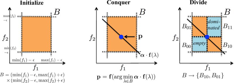
PEPFR divide-and-conquer approach for identifying the Pareto frontier, illustrated for two objectives. (Initialize) The boundaries of an initial box are defined by separately minimizing and maximizing f1 and f2. (Conquer) The box-constrained optimizer g produces a Pareto optimal design λ within the current box B, using weights α on the two objectives. (Divide) The current box B is divided into four sub-boxes according to the design λ determined in the conquer step. B00 and B11 are discarded, and the algorithm recurses independently with B10 and B01.
Initialize
Each of the two objectives is separately minimized and also maximized (i.e., its negative is minimized), using the optimizer g with the single objective over the entire objective space. In our presentation, we define all the boxes to be open, not containing the boundaries. To be consistent with that, we relax the determined minimum and maximum values with a tiny value ε, to yield an open box B = (min(f1) −ε, max(f1) + ε) × (min(f2) − ε, max(f2) + ε).
Conquer
The box-constrained optimization algorithm g is applied to find the optimal design λ within the current box B, under a set of coefficients α to linearly combine the objectives. We can prove (see Supplementary Material) that this design is in fact undominated within B. Since, as we discuss more in the “divide” step, no design in any other box dominates any design in B, it then follows that λ is Pareto optimal.
Divide
Let λ be the undominated design uncovered in the box B = (l1, u1) × (l2, u2) during a conquering step. Let p = (p1, p2) = f(λ). We use p to divide B into four rectangular portions, excluding points on the two lines x = p1 and y = p2 because they are dominated by p. We name the regions B00, B01, B10, and B11, where the subscript 0 denotes (li, pi) and 1 denotes (pi, ui); since li < pi < ui, the naming is consistent with the geometry. Since p is undominated in B, no design is in B00, otherwise it would dominate p, a contradiction. Furthermore, p dominates all the points in B11. Therefore, both B00 and B11 can be pruned, and we recurse in B01 and B10. Note that B10 has a better range in the second dimension while B01 has a better range in the first dimension, so points in one cannot dominate those in the other. They therefore can be recursively explored independently and their undominated designs simply unioned together.
The algorithm recurses twice (once for each sub-box) for each Pareto optimal design added to F; a recursion terminates upon discovering an empty box. Thus the algorithm can be viewed as having an “output sensitive” complexity, in that the cost is proportional to the size of the output. More specifically, the underlying optimizer g (whose computational complexity we don’t know) is invoked 2|F| + 1 times. Thus the total time required is O(Ft) if t bounds the time required by g.
2.2 Instantiations of the box-constrained optimizer
We show how to instantiate the box-constrained optimization algorithm g for approaches employing integer programming or dynamic programming, two common optimization techniques in protein engineering.
2.2.1 Integer linear programming (IP)
Integer programming is a powerful optimization technique applicable to a number of NP-hard optimization problems including protein engineering. NP-hardness implies that both efficiency and optimality cannot simultaneously be guaranteed. Here we choose to guarantee optimality, and use the state-of-the-art solver CPLEX that typically works quite efficiently in practice. An integer program is specified in terms of a set of integer (often binary) variables, an objective function that is a linear combination of the variables, and a set of constraints on the values of the variables:
Variables vector x, with xi an integer
Objective minimize c · x
Constraints such that Ax ≤ b
To make this more concrete, let us consider a generic site-directed mutagenesis experiment; we will instantiate later for specific objectives. The variables represent the entire amino acid sequence (including both wild-type and substituted positions): binary variable xik ∈ {0, 1} indicates whether or not residue position i is of amino acid type k, with i ranging over the entire sequence and k over the amino acid types allowed at position i. The objective function expresses the contribution of each possible amino acid type at each position, weighting xik by a coefficient cik. Thus x effectively serves as a mask, with only those variables that end up being set to 1 actually adding to the score. Constraints ensure that there is a single amino acid type at each position. For example, one row in A would ensure that the sum of x1k (all the amino acid types at position 1) is at least 1, while another row would ensure that it is at most 1, and similarly for other positions. Additional constraints can also limit the total number of substitutions, etc.
In our PEPFR framework, we need to optimize a weighted combination of the design objectives, α · f(λ), within a box B. We represent λ with x, and each objective fi as a set of coefficients ci on the values in x. Then c is an α-weighted sum of these coefficients, α1c1 + α2c2. Finally, to focus on a box B = (l1, u1) × (l2, u2), we add constraints such that l1 < c1 · x < u1 and l2 < c2 · x < u2.
2.2.2 Dynamic programming (DP)
Dynamic programming (DP) is another standard combinatorial optimization technique, also applicable to protein engineering problems. In contrast to integer programming, it can guarantee both optimality and efficiency, but is only suitable in a more limited range of scenarios in which a problem can be decomposed into subproblems such that the optimal solution to the original problem is determined from the optimal solutions to subproblems. It is naturally applicable to protein engineering problems that can be decomposed in sequential order, proceeding from the N-terminus to the C-terminus (in the same way as the well-known pair-wise sequence alignment algorithms).
Dynamic programming is a general technique, so for the sake of concreteness, we describe here one particular formulation suitable for protein engineering. This formulation can readily be extended or adapted for other protein engineering problems. We use one variable to represent progress through the sequence (from N- to C-terminus) and another variable to represent progress through the different design parameters (breakpoints or mutations) for which values must be chosen. Thus D(r, k) represents a design for the first r residues and the first k parameters; in fact, we define it such that the kth choice is made exactly at position r. For example, D(200, 5) represents the best design placing 5 breakpoints or mutations within the first 200 residue positions, with the 5th at 200. A recurrence expresses the best score (α-weighted sum of design objectives) attainable for an (r, k) design based on the best score attainable for sub-designs. For recombination design and for mutation design when treating mutations additively, the sub-designs are those for previous positions r′ < r where the (k − 1) choice could be made, and the recurrence takes the form
| (1) |
incrementing the score of the (r′, k − 1) design by the score contribution Δf due to the additional design choice.
Dynamic programming computes the recurrence by starting from trivial subproblems and building up solutions to increasingly larger subproblems, using a table to keep track of the solutions (since they may be used by multiple super-problems). Thus we fill in a table of D(r, k) values with an inner loop from the N-terminus to the C-terminus and an outer loop from the first breakpoint or mutation to the last. In addition to the optimal score, we keep track of the choice made to obtain it (which r′, which substitution). Then the optimal overall design can be obtained by backtracing from the best cell for the final design choice (which could be at any residue position), moving recursively back through the predecessors to the first design choice.
While PEPFR requires the ability to find an optimal solution within a particular box, standard dynamic programming can yield an optimal solution anywhere in the design space. Thus to use DP as our box-constrained optimizer, we have developed a new backtracing algorithm (analogous to algorithms for finding near-optimal solutions in a DP table [1, 63]) that performs a tree search to identify an optimal design within a given box. While a regular backtrace produces a single path by following the best predecessor from each cell, our backtrace produces a tree of paths by following all predecessors of a cell. (Note that a cell can be reached by multiple paths.)
When reaching a cell, there are three possibilities: stop if we have found a design within the box; prune if we are guaranteed not to find an optimal solution within the box along this path; else branch to continue exploring predecessors. To be able to make the decision, we need the following information (Fig. 3):
o: the optimal value of α · f(λ) within B found so far. This is initialized to a large value and minimized during the algorithm.
b(P, r, k): the vector of contributions to f back along path P from a terminal cell to cell r, k. This is tallied in the process of building P, incrementing by Δf each step.
d(r, k): the vector of contributions to f forward from an initial boundary cell to cell r, k. We extend the regular DP computation to maintain this information for each cell, by simply adding Δf to the d(r′, k − 1) vector for the optimal predecessor.
- : the range of f values achieved over any path from an initial boundary cell to cell r, k. This requires filling in additional DP tables with recurrences to maintain the lower (L) and upper (U) bounds on the different objectives (i):
(2)
and then computing , U1(r, k) + b1(P, r, k)) × (L2(r, k) + b2(P, r, k), U2(r, k) + b2(P, r, k)).(3)
Figure 3.
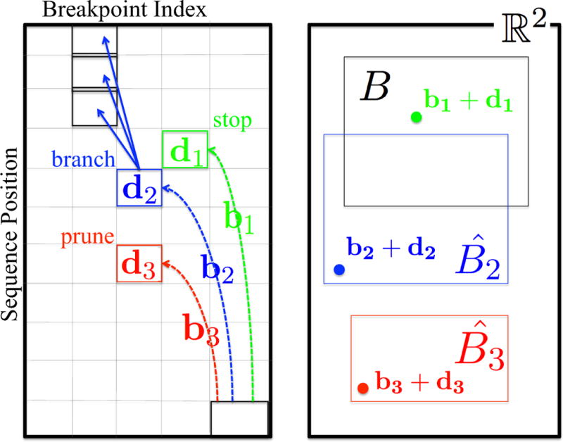
Backtrace for box-constrained optimization by dynamic programming. (left) The dynamic programming table. Different paths from the final cell (lower right) have been followed back to three different cells, marked with different colors and subscripts. (right) The objective space, showing the contributions to f of the optimal designs and bounds on the values for the three different cells reached by the three different paths, using corresponding colors and subscripts (instead of the parameters to b, d, and ). The desired box is B. The design for cell 1 is in B, so we stop and see if it is the best so far. The design for cell 3 is in , guaranteed to be outside of B, so we prune the cell. The design for cell 2 is in , and thus may or may not be in B, so we must continue backtracing from the cell.
Then when reaching cell r, k on backtracing path P, we use this information to decide how to proceed:
prune if , as this path will not lead to any solution in the box
stop if d(r, k)+b(P, r, k) ∈ B; then compare α·(d(r, k)+b(P, r, k)) against o, and keep the better solution
branch otherwise
To implement the backtracing algorithm, we maintain a priority queue of active paths. The priority is set by α · (b(r, k) + d(P, r, k)), based on the usual heuristic that a path with a better combination of score so far plus bound on remaining score is more likely to lead to a suitable design faster, and thus provide better pruning power via o. The queue starts with the trivial path(s) containing the terminal cell(s) in the dynamic programming matrix. When a path is to be branched, it is extended by each possible predecessor, and the resulting paths added to the queue. The search continues until the queue is empty.
2.3 Case studies
To illustrate the power and generality of PEPFR, we instantiate it for three protein engineering problems for which other techniques have previously been applied in order to optimize competing objectives. We here briefly motivate these studies and summarize their formulations in PEPFR.
2.3.1 Therapeutic protein deimmunization
Protein therapeutics derived from exogenous sources have a high risk of eliciting an immune response in human patients [25], mitigating the therapeutic benefits and potentially even yielding detrimental effects including anaphylactic shock [50]. Deimmunization seeks to modify a protein so that it does not produce an immune response yet still is an effective therapeutic. While therapeutic antibodies have been successfully deimmunized by techniques leveraging their particular structure and function [38, 21, 64], other classes of proteins (e.g., enzymes, receptors, and binding proteins) still pose significant challenges for deimmunization. One generally applicable approach, epitope deletion, has been successfully applied to several therapeutic candidates including staphylokinase [62], erythropoietin [57], and factor VIII [22]. The key idea [6] is to identify immunogenic peptide fragments, or epitopes, within the protein, and mutagenize key residues so as to disrupt the fragments’ ability to complex with type II major histocompatability complex (MHC II) proteins and/or T-cell receptors. By disrupting the formation of a ternary peptide-MHC II-T-cell receptor complex, the immune response is forestalled.
Parker et al. [43] recently developed a computational approach called IP2 to optimize site-directed mutations for protein deimmunization, in order to delete T-cell epitopes while maintaining therapeutic activity. These two objectives are competing, as structurally and functionally conservative mutations may not help in reducing immunogenicity, while effective mutations for deimmunization may be structurally and functionally disruptive. The deimmunization objective is assessed by sequence-based T-cell epitope predictors, which encapsulate the specific recognition of peptides by MHC II proteins. Numerous such predictors have been shown to be predictive of immunogenicity and employed in analysis and design contexts [55, 52, 40, 8, 39, 61, 7]. An epitope predictor is packaged up in a function e that takes a 9-mer peptide and returns an epitope score, with lower numbers for less immunogenic peptides. The stability/activity objective is assessed with one-body and two-body sequence potentials that capture position-dependent residue conservation and co-variation from a multiple sequence alignment of homologs to the target. Such potentials, which have been essential in other protein engineering contexts [60, 46, 53], take advantage of the fact that constraints on amino acid choices required to maintain structure and function are likely to be manifested in the sequence record. These potentials are represented as negative logs, so that lower is better, and denoted ϕi(a) for amino acid type a at position i, and ϕi,j(a, b) for types a, b at positions i, j.
As we discussed, an integer program (IP) is specified in terms of integer variables, a linear objective function, and a set of linear constraints. Parker et al. employed three types of binary variables: singleton binary variables si,a indicating whether or not position i has amino acid type a, pairwise binary variables pi,j,a,b indicating whether or not positions i, j have respectively amino acids types a, b, and window binary variables wi,X, indicating whether or not the 9-mer starting at position i has the 9 amino acid types in order in X. The deimmunization objective function (“epitope score”) is the sum of the scores for all the constituent 9-mers of the protein, with the w variables essentially masking which peptides actually contribute:
| (4) |
The stability/activity objective function (“sequence score”) similarly sums the potential functions over all positions and pairs of positions, using the s and p variables as masks:
| (5) |
The constraints then ensure a single amino acid type at each position (Eq. 6), consistency of the single and pairwise variables (Eqs. 7 and 8), consistency of the single and window variables (Eq. 9), and that the desired number of mutations is made relative to the wild-type sequence S (Eq. 10):
| (6) |
| (7) |
| (8) |
| (9) |
| (10) |
To perform optimization constrained to box B = (l1, u1) × (l2, u2), we add the constraints we previously described: l1 < f1 < u1 and l2 < f2 < u2.
While Parker et al. manually sampled relative weights α1 and α2 between the two objectives, our divide-and-conquer approach is able to find all Pareto optimal designs by using this IP for the box-constrained optimizer g, and a fixed choice for α (we used (1,1) for the results given).
2.3.2 bZIP partners
Protein-protein interactions play important roles in numerous biological processes, and have been the focus of much significant protein design work for both strength and specificity [34]. Grigoryan et al. [11] targeted human basic-region leucine zipper (bZIP) transcription factors, as human bZIP proteins participate in a wide range of important biological processes and pose attractive targets for selective inhibition. They developed a computational approach for designing bZIPs that successfully designed synthetic interacting bZIP peptides with desired interaction strength and specificity. The strength and specificity goals are competing, as strength against the target may have to be sacrificed in order to obtain specificity, and similarly a very specific but low-affinity binder is not desirable.
In order to assess the strength and specificity of a designed interaction, Grigoryan et al. used “cluster expansion” to truncate their previously-developed structurally-based bZIP interaction energy functions [12], yielding position-specific single-position and pairwise energy terms that depend only on amino acid type and may be linearly combined. Interaction strength is evaluated as the design:target energy and interaction specificity as the minimum gap between the design:target energy and all design:competitor energies (including off-target bZIPs and the homo-dimer). The interacting proteins are represented as an undirected p-partite graph (for a designed protein of length p) with position-specific sets Vi of nodes for the allowed amino acid types at position i, and edges D = {(u, v): u ∈ Vi, v ∈ Vj, i ≠ j} between all pairs of amino acid nodes at different positions.
They then developed an IP-based optimization approach called CLASSY, as usual specifying variables, an objective, and a set of constraints. Two types of binary variables are employed: singleton binary variables xuu representing the amino acid choice at node u, and pairwise binary variables xuv representing the pair of amino acid choices for edge (u, v). The design:target objective is the total energy:
| (11) |
where is the single-position energy term for node u (one of the amino acid choices at a position), and similarly is the pairwise energy term between nodes u and v. The strength against competitor c (from the set of k competitors, including the homodimer) has a similar form. While Grigoryan et al. use it in a constraint, we view it as a competing objective:
| (12) |
and show below how to handle the fact that each competitor results in such an objective.
The constraints then ensure the choice of single amino acid type at each position (Eq. 13), match choices of pairwise binary variable with corresponding singleton binary variables (Eq. 14), enforce a “PSSM score” threshold to favor a leucine-zipper fold based on consistency with sequence statistics in a multi-species bZIP alignment (Eq. 15), and enforce a minimum energy gap between the design:design energy and each design:competitor energy (Eq. 16).
| (13) |
| (14) |
| (15) |
| (16) |
Grigoryan et al. employed a “specificity sweep” approach, first identifying the design with the strongest binding strength, noting its energy gap, running the IP again using that gap as a constraint in order to find a design with a better gap (but worse strength), and repeating to incrementally increase the gap. We instead seek to find all Pareto optimal points by applying our divide-and-conquer approach based on this underlying optimizer.
To use this integer program in PEPFR, we need an objective combining the strength (f1 target energy) and the specificity (gaps between f1 and the various f2,c off-target energies). We treat each competitor separately, essentially assuming it has the smallest gap, and run k different IPs for the different competitors, each extended from the above IP. The extended IP for competitor c has the objective α1f1 + α2(f1 − f2,c), with specificity inverted to be consistent with our minimization convention. It incorporates the additional specificity constraint
| (17) |
and the usual box constraints l1 < f1 < u1 and l2 < f1 − f2,c < u2. The minimum value of α · f is the minimum of the integer programming objective over the k different runs.
2.3.3 Site-directed recombination
Site-directed recombination generates a library of hybrid proteins from homologous protein parents, mixing-and-matching fragments in seeking to uncover new combinations with improved function [60]. In contrast with stochastic recombination (natural or in vitro), site-directed recombination allows the breakpoints to be specified, based on an analysis of which are likely to yield beneficial hybrids. In contrast with mutagenesis, site-directed recombination employs amino acid combinations that have been evolutionarily accepted in the same structural context, and thus are likely to yield viable proteins. Site-directed recombination has been successfully applied to develop variant enzymes with improved properties and activities [36, 9, 42, 35, 41, 30, 32, 19, 18].
Zheng et al. [67] developed a Pareto optimization approach called STAVERSITY to optimize site-directed recombination experiments according to two criteria: whether the hybrids are likely to be stable and active and how diverse the library is. These are competing goals, as in order to produce stable, active hybrids, the best strategy is to cluster the breakpoints at the termini, yielding hybrids that closely resemble the parents. The stability/activity objective evaluates the expected sequence-structure “perturbation” in the hybrids relative to the parents, according to the potential developed by Ye et al. [65] This potential, like other similar ones [60, 37, 47, 9], is based on correlation statistics between interacting residues, recognizing that recombination potentially disrupts the pairwise interactions underlying stable folding. While Ye et al. considered up to 4-residue interactions, we focus here only on pairwise interactions. In this case, the perturbation score between a set P of parents and set H of hybrids is:
| (18) |
where i and j are contacting residue positions and a and b are amino acid types there, and ϕi,j(a, b) is the potential score. Ye et al. showed how to compute f1 efficiently, without actually having to enumerate all the hybrids in the library [65].
The diversity objective evaluates the overall “mutational variance” within the library [68]. Minimizing the variance seeks a relatively uniform sampling of the design sequence space, and thus improves the chances of finding a novel variant. Diversity had been optimized only indirectly in earlier work, though others had found it to be important in development of beneficial hybrids. The diversity variance is:
| (19) |
where the indicator function I returns 1 when hybrid Hi and parent Pa have different residues. To ignore conservative substitutions, “equality” is evaluated according to standard amino acid classes {{C},{F,Y,W},{H,R,K},{N,D,Q,E},{S,T,P,A,G}, {M,I,L,V}}. As with perturbation, we do not actually have to enumerate the hybrids to compute the diversity variance [68].
Perhaps surprisingly, given that the perturbation computation includes long-range pairs of contacting residues (including those spanning breakpoints), a polynomial-time dynamic programming algorithm is applicable for each objective and there are recurrences to compute the incremental perturbation and variance due to adding one more breakpoint. While the actual formulas are quite detailed [67], the structure of the dynamic program is exactly like the one we presented. The STAVERSITY algorithm of Zheng et al. [67] finds some of the Pareto optimal points based on this dynamic program. PEPFR finds all of them, when using the same DP formulation combined with our new back-trace algorithm within our divide-and-conquer framework.
3 Implementation
PEPFR is implemented in standard C++, compilable by the GNU compiler. As a “meta-design” algorithm, it is developed in a modular fashion, with classes for the box-constrained optimizers and objective functions. We provide optimizer classes encoding our integer programming and dynamic programming approaches. For IP, the optimization is performed by calls to CPLEX via its C++ API. We directly implement a standard DP recurrence and our custom backtrace. We provide objective function classes for the various metrics used in the case studies. Auxiliary classes handle input data (e.g., multiple sequence alignments, epitope scoring matrices, position-specific scoring matrices) to compute the various potential scores.
Our source code is freely available for academic use, at http://www.cs.dartmouth.edu/~cbk/pepfr/.
4 Results and Discussion
We now demonstrate the effectiveness of PEPFR in discovering the Pareto frontier for our three case studies. For each, we are able to incorporate the published objective functions (and their parameters) into PEPFR and thereby directly compare our designs with those previously determined. In addition to finding all the Pareto optimal designs found by the earlier methods, we find a large number of new designs and demonstrate that some previously determined designs were not Pareto optimal.
The CPU time required by PEPFR is case-specific; as discussed, it is directly related to the number of outputs and the cost of the underlying optimizer. The optimization cost can in turn depend on the density of points designs near the Pareto frontier, as well as the α coefficients (which we fix at (1, 1) here). The following results were collected on a single core machine, and most runs required minutes to hours of wall-clock time, though the range spanned from seconds (2-breakpoint recombination design) to a few days (9-breakpoint recombination designs). The expense of the 9-breakpoint optimization was due largely to the sheer density of points in one region of the space. While that amount of time for planning seems acceptable, the approach could readily be parallelized to reduce the required wall-clock time if that were desired in some context.
4.1 Therapeutic protein deimmunization
Parker et al. applied their IP2 deimmunization method to several different therapeutic proteins, identifying sets of mutations predicted to be both deimmunizing and function-preserving [43]. We examine here erythropoietin (Epo), peptides from which had previously been experimentally targeted by Tangri et al. [57] We instantiated the objective functions as described by Parker et al. For the epitope score (Eq. 4), we compute the number of the 8 most abundant MHC-II alleles [54] predicted to bind a peptide according to ProPred [52] at a 5% threshold. For the sequence score (Eq. 5), we compute one- and two-body potentials from the Pfam-curated MSA (id PF00758), after removing sequences with less than 35% or more than 90% identity to the target. We consider mutations appearing in at least 5% of the remaining sequences; while one might typically want to eliminate Cys and Pro substitutions, we did not do so here in order to render our results directly comparable.
We generated the Pareto frontier at a number of different mutation loads. Fig. 4 illustrates the scores of 4-mutation and 8-mutation designs identified by PEPFR, along with those sampled by Parker et al. For 4 mutations, PEPFR identified 24 Pareto optimal designs, while for 8, it identified 40. In both cases, Parker et al. sampled only 6 designs by varying the relative weight between the two objectives. As Fig. 4 shows, one of the 4-mutation designs is not Pareto optimal; we believe this to be due to the setting of a parameter controlling which substitutions are considered. Following the Pareto frontiers from right to left (with decreasing immunogenicity), we see a smooth decrease in epitope score with relatively little penalty in sequence score, until reaching a “knee” at which point progress in immunogenicity requires substantially less conservative substitutions. PEPFR fully elucidates the set of Pareto optimal designs around that knee. Studying the trade-offs made along the frontier helps the engineer calibrate the price that must be paid on one objective in order to make gains on the other.
Figure 4.
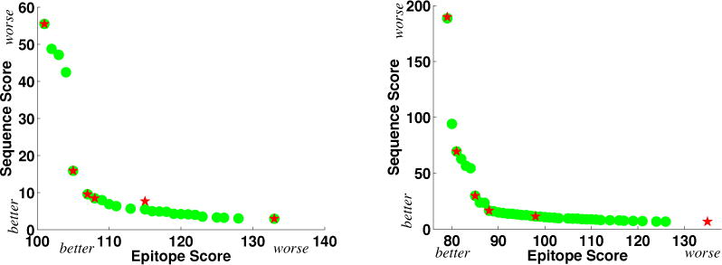
Pareto frontiers for (left) 4-mutation and (right) 8-mutation Epo deimmunization designs (x: epitope score; y: sequence score). Green dots: Pareto optimal designs discovered by PEPFR; red stars: designs (not necessarily Pareto optimal) sampled by Parker et al. [43]
Fig. 5 illustrates one of the 8-mutation designs (epitope score 88) near the knee in the Pareto frontier. We see that each mutation is effectively employed to reduce epitopes and no new epitopes are introduced. While some of our mutations focus on the immunogenic peptides experimentally targeted by Tangri et al. [57], PEPFR is a global design method allowing mutations throughout the protein and evaluating their predicted impacts on both epitope and sequence scores. Thus it also picks up additional promising-looking mutations in other regions of the protein. It also simultaneously considers each residue in each MHC frame (not just as, say, the P1 anchor). It can more confidently propose higher mutational loads by explicitly evaluating the relative conservativeness of substitutions (including their interaction terms).
Figure 5.
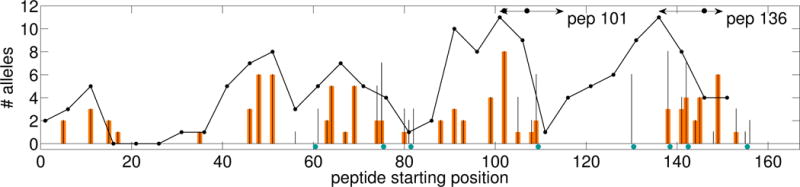
Epitope profile (following Parker et al. [43]) of a selected Epo 8-mutation Pareto optimal design identified by PEPFR. x-axis: starting position of each 9-mer; y-axis: predicted number of alleles recognizing the 9-mer. Thin black bars indicate wild-type scores and thick orange bars indicate variant scores. Note: wild-type epitope scores are always greater than or equal to corresponding variant ones; i.e., no new epitope is introduced. Blue circles indicate mutated positions. Black ellipses at top indicate Tangri et al. [57] mutated positions. The line plot, from Tangri et al., displays wild-type Epo antigenicity using ELISPOT assays, with black dots giving the number of alleles bound to overlapping 15-mers; it trends very well with the ProPred-predicted epitopes.
One of the benefits of elucidating the entire Pareto frontier is the resulting ability to track trends in mutations, as we trade off between one objective and the other. Fig. 6 shows the mutation profile of the 8-mutation Epo Pareto frontier, from least immunogenic but least conservative (top) to most conservative but most immunogenic (bottom). We see the trade-off between placing mutations in the more immunogenic regions (though not necessarily at the initial residues of immunogenic peptides), near the top, and employing more conservative mutations, near the bottom. We also see some “popular” mutations employed over long stretches of the Pareto frontier; these may combine the best of both worlds. The trend analysis also helps in identifying a small number of relatively different plans for additional modeling and ultimately experimentation.
Figure 6.
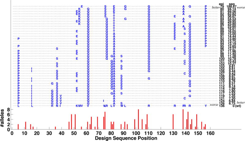
Mutation profile for Pareto frontier of Epo 8-mutation designs. Each design is represented as a dashed line marked with mutations; the bottom row shows the corresponding wild-type residues. Designs are ranked from top to bottom as increasing epitope score and decreasing sequence score (values are on the right). The wild-type epitope profile is provided at the very bottom, with red bars indicating the number of alleles for each starting 9-mer position.
4.2 bZIP partners
Grigoryan et al. computationally developed (using Classy) and experimentally evaluated synthetic partners for 46 different human bZIPs (nearly all human bZIPs) [11]. We consider here one representative (and well-characterized) target, MafG, an oncoprotein involved in regulating cell differentiation and other cellular functions [20]. We apply PEPFR to design anti-MafG partners that are predicted to be both strong and specific binders, preferring MafG to 45 other human bZIPs from the 20 different families of human bZIPs, as well as to the design:design homodimer. We adopt the energy model used by Grigoryan et al., including values for the energies Euu and Euv (Eqs. 11 and 12). In this model, only four positions (a, d, e, and g) of the bZIP heptad repeat contribute to the energy. Following Grigoryan et al., we selected amino acids for the other positions by maximizing likelihood based on frequencies in a multi-species dataset of 432 bZIP sequences.
Fig. 7 shows the PEPFR Pareto frontier, along with the designs identified by the Classy method of Grigoryan et al., in both our objective space representation and their specificity sweep representation. We find 108 designs, of which they identified 35. Relative specificity is better further to the left in our representation, and to the right in theirs (with an increasingly positive gap between target stability and off-target stability). The design:design homodimer interactions tend to be the strongest competitors for the Pareto optimal anti-MafG designs; we see from the bottom figure that for the most of designs, the design:design homodimer (back squares) has the smallest energy gap with the design:target heterodimer. We see a relatively smooth trade-off of stability for specificity (moving left in our representation and right in theirs), though there is a clearly evident “knee” in our representation where we must begin to pay a much larger penalty for stability in order to gain additional specificity. Notice that PEPFR has a much denser set of designs with good specificity. By characterizing all the designs, PEPFR elucidates the relative value and cost of the two competing factors, and provides more opportunity to identify the most beneficial ones for experimental evaluation, as well as additional designs with very similar properties if alternatives are needed.
Figure 7.
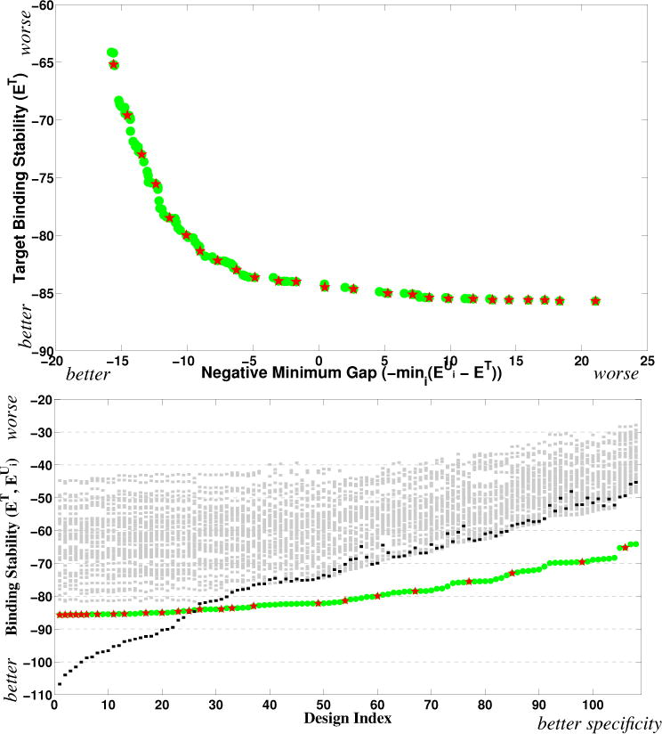
Anti-MafG Pareto frontier, with the PEPFR designs plotted as green dots and those of Grigoryan et al. [11] as red stars. (top) Objective space representation, with x for specificity and y for stability. (bottom) Specificity sweep representation of Grigoryan et al. The y-axis indicates binding stability values; the designs are sorted in x in order of their binding specificity (minimum gap). In addition to the design:target stability values (green dots and red stars), the design:off-target values are shown with gray squares and the design:design values with black squares.
Fig. 8 profiles the amino acid content of the anti-MafG designs. Inspection of nearby designs allows us to assess the key determinants of their stability and specificity, and alternatives with similar properties. For example, consider the design at index 60 in Fig. 8, which was selected by Grigoryan et al. for experimental characterization. We see that many of the amino acid choices in this design (of those that vary from the baseline most stable design at index 1) are common nearby in the Pareto frontier. Furthermore, much of the variability is fairly conservative, e.g., K or R at e4, V or L at a5, and D or E at g7. As a result, the objective scores (Fig. 7, top) remain fairly constant locally. Interestingly, we see the emergence of N at a1 in this neighborhood, a mutation that is preserved from that point on for better specificity (a large number of off-targets have A, T, I, L, or V at a1′, undesirable for interactions with N). Furthermore, there is a set of mutations that consistently distinguish this neighborhood from the most stable designs (e.g., g2 is now K instead of I, g3 is now R instead of D, and e5 is now R or E instead of L) and from the most specific ones (e.g., d3 is still L instead of K, e4 is still R or K instead of A, and a5 is still L or V instead of R).
Figure 8.
Amino acid content along the Pareto frontier of anti-MafG bZIP peptide designs. Rows: amino acid positions, grouped by heptad from top to bottom, showing only the optimized heptad positions g, a, d, and e. Columns: MafG sequence (leftmost, in red) and designs, from most stable (left) to most specific (right), using the same indices as in the bottom of Fig. 7. The full sequence is shown for the most stable design; only differences are shown for the others.
Further characterizing entire portions of the design space allows us to see trends underlying the trade-off between stability and specificity. For example, the first 26 designs are not specific, and in fact prefer to homodimerize rather than bind MafG (see again Fig. 7, bottom). In Fig. 8, we see that, compared to the most stable design, these designs primarily make substitutions at heptad positions g and e. Grigoryan et al. also noticed that their method initially improved specificity by modulating electrostatic g-e’ interactions (i.e., the g in one heptad and the interacting e in the next). We often observe E-E and K/R-K/R pairs at g-e′, yielding like charges in the homodimer, increasing its energy; these same positions yield only one undesirable R-K pair in the design:target heterodimer, leaving its energy practically the same. Following these first 26 nonspecific designs, we begin to see more substitutions modulating the g-a’ and a-d interactions, to further destabilize the design:design homodimer. We observe many of the characteristics of designs that are disruptive to homodimers, as summarized by Grigoryan et al., including like charges in g-a′ interactions (e.g., E-E at g5-a6) and pairs of beta-branched residues in a-d’ interactions (e.g., I-V in a6-d6 and a7-d7). Finally, we see characteristics stabilizing the design:target heterodimer, including paired L at d and paired N at a.
4.3 Site-directed recombination
We apply PEPFR to optimize site-directed recombination designs for beta-lactamases, enzymes that hydrolyze the beta-lactam in various antibiotics including penicillins and cephalosporins. Beta-lactamases have previously been the targets of site-directed recombination [36, 9, 35, 65], including as a case study for the STAVERSITY approach of Zheng et al. [67] Following that case study, we also target parents TEM-1 and PSE-4, and derive a sequence potential from the same set of 136 beta-lactamases multiply aligned to 263 residues (average sequence identity: 41.8%), limiting the two-body terms to pairs of residues within 8 Å in the TEM-1 structure (pdb id: 1btl). As discussed in the methods, we only use one- and two-body potentials, while Zheng et al. also used three- and even four-body potentials; thus for comparison, we re-ran their method with only the one- and two-body potentials.
Fig. 9 illustrates the Pareto frontier identified by PEPFR, along with the scores of the designs identified by re-running STAVERSITY. For each score, there are multiple designs producing that score (e.g., by sliding a breakpoint left or right in homologous regions). PEPFR identifies all such designs. In all three cases, as we follow the Pareto frontier from left to right, we see an initial sharp drop of perturbation score with relatively little penalty of diversity variance until reaching a “knee”. After that point, there is a relatively smooth decrease of perturbation score but a sharp increase in diversity score, finally ending with several jumps. For 2 breakpoints, PEPFR identified 45 distinct Pareto optimal points, and STAVERSITY identified the same number. For 6 breakpoints, PEPFR identified 203 distinct Pareto optimal points; STAVERSITY identified 154 distinct points, 10 of which are not actually Pareto optimal. For 9 breakpoints, PEPFR identified 257 distinct Pareto optimal points, while STAVERSITY identified 174 distinct points, including 17 that are not Pareto optimal. Thus while the PEPFR and STAVERSITY curves look similar to the eye, STAVERSITY actually missed 59 of the 203 6-breakpoint plans and 100 of the 257 9-breakpoint plans.
Figure 9.
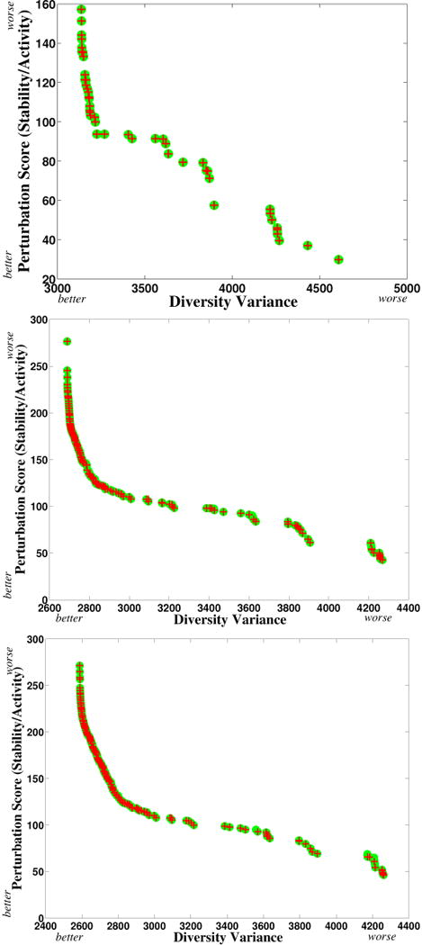
Pareto frontier for (top) 2-breakpoint, (middle) 6-breakpoint, and (bottom) 8-breakpoint beta-lactamase designs (x-axis: diversity; y-axis: perturbation). Green dots: Pareto optimal designs discovered by PEPFR; red crosses: designs (not necessarily Pareto optimal) sampled by the STAVERSITY method of Zheng et al. [67]
Fig. 10 illustrates the breakpoint selections along the Pareto frontiers. Going from top to bottom in each panel, we see that the best libraries in terms of perturbation cluster the breakpoints near the N-terminus (leaving the hybrids largely the same as the parents), while the best libraries in terms of diversity spread the breakpoints out more evenly. We also see some “hot spot” locations where breakpoints are frequently placed and persist over large ranges of perturbation and diversity scores; these locations seem to lead to beneficial hybrids under both objectives. Reference to the secondary structure elements does not reveal any clear pattern of preference for placement of breakpoints within or between them.
Figure 10.
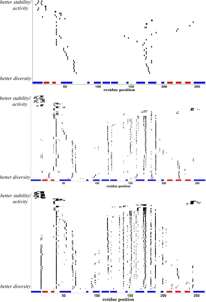
Designs along the Pareto frontier of beta-lactamase site-directed recombination designs, for (top) 2, (middle) 6, and (bottom) 9 breakpoints. In each panel, columns represent residue positions and rows represent designs by marking the breakpoint locations; rows are ordered from best according to structural perturbation (top) to best according to diversity (bottom). The secondary structure according to the TEM-1 structure (pdb id:1btl) is shown at the bottom of each panel, with blue boxes for α-helices and red boxes for β-sheets.
5 Conclusion
We have presented a new approach to balancing competing objectives in rational protein engineering, generating the complete Pareto optimal frontier in order to enable characterization of local and global trends and selection of the most beneficial experimental designs. In contrast to earlier methods for optimizing multiple objectives in protein engineering, our PEPFR method is guaranteed to find all Pareto optimal designs. While algorithms for Pareto optimization have also been developed in support of other applications (e.g., see the survey by Handl et al. on approaches in computational biology [15]), the most common techniques include sampling relative weights (as previously discussed) and performing a heuristic search (e.g., genetic algorithms). Unfortunately, such techniques cannot provide any guarantees of correctness and may miss important points or even regions of the Pareto frontier. Before performing costly experiments, it is worth fully characterizing the trade-offs that must be made between the competing objectives. In the context of rational protein engineering, completeness implies that experimental outcomes can be directly tied back to the models underlying the optimization, without worrying about artifacts from the optimization algorithm. Assessing the local and global trends in designs (persistence of design choices) can also help better assess the likelihood of success of an experiment. As we showed with three quite different case studies, PEPFR is very general, supporting powerful integer programming and dynamic programming optimization techniques to select mutations or breakpoints. It remains future work to integrate other design techniques (e.g., dead-end elimination [5] and RosettaDesign [28]) within the framework. PEPFR provides the protein engineer with a powerful mechanism for developing robust, diverse, high-quality experimental plans.
Supplementary Material
Acknowledgments
This work was supported in part by US NSF grant IIS-1017231 and US NIH grant R01GM098977. We gratefully acknowledge help with the case studies (including data, code, and discussion) from Andrew Parker, Gevorg Grigoryan, and Wei Zheng.
Footnotes
Since it uses divide and conquer, the full name of our approach is DRPEPFR, but we use PEPFR more informally.
References
- 1.Bellman R, Kalaba R. On the Kth best policies. J SIAM. 1960;8:582–588. [Google Scholar]
- 2.Bolon DN, Grant RA, Baker TA, Sauer RT. Specificity versus stability in computational protein design. PNAS. 2005;102:12724–12729. doi: 10.1073/pnas.0506124102. [DOI] [PMC free article] [PubMed] [Google Scholar]
- 3.Carbone MN, Arnold FH. Engineering by homologous recombination: exploring sequence and function within a conserved fold. Curr Opin Struct Biol. 2007;17:454–459. doi: 10.1016/j.sbi.2007.08.005. [DOI] [PubMed] [Google Scholar]
- 4.Carter CW, Jr, LeFebvre BC, Cammer SA, Tropsha A, Edgell MH. Four-body potentials reveal protein-specific correlations to stability changes caused by hydrophobic core mutations. J Mol Bio. 2001;311:625–38. doi: 10.1006/jmbi.2001.4906. [DOI] [PubMed] [Google Scholar]
- 5.Dahiyat BI, Mayo SL. De novo protein design: Fully automated sequence selection. Science. 1997;278:82–87. doi: 10.1126/science.278.5335.82. [DOI] [PubMed] [Google Scholar]
- 6.De Groot AS, Knopp PM, Martin W. De-immunization of therapeutic proteins by T-cell epitope modification. Dev Biol (Basel) 2005;122:171–94. [PubMed] [Google Scholar]
- 7.De Groot AS, Martin W. Reducing risk, improving outcomes: Bioengineering less immunogenic protein therapeutics. Clinical Immunology. 2009;131:189–201. doi: 10.1016/j.clim.2009.01.009. [DOI] [PubMed] [Google Scholar]
- 8.De Groot AS, Moise L. Prediction of immunogenicity for therapeutic proteins: State of the art. Curr Opin Drug Discov Devel. 2007;10:332–340. [PubMed] [Google Scholar]
- 9.Endelman JB, Silberg JJ, Wang ZG, Arnold FH. Site-directed protein recombination as a shortest-path problem. Protein Eng Des Sel. 2004;17:589–594. doi: 10.1093/protein/gzh067. [DOI] [PubMed] [Google Scholar]
- 10.Godfrey P, Shipley R, Gryz J. Maximal vector computation in large data sets. Proc VLDB. 2005:229–240. [Google Scholar]
- 11.Grigoryan G, Reinke AW, Keating AE. Design of protein-interaction specificity gives selective bZIP-binding peptides. Nature. 2009;458(7240):859–864. doi: 10.1038/nature07885. [DOI] [PMC free article] [PubMed] [Google Scholar]
- 12.Grigoryan G, Zhou F, Lustig SR, Ceder G, Morgan D, Keating AE. Ultra-fast evaluation of protein conformational energies directly from sequence. PLoS Comput Biol. 2006;2:e63. doi: 10.1371/journal.pcbi.0020063. [DOI] [PMC free article] [PubMed] [Google Scholar]
- 13.Gronwald W, Hohm T, Hoffmann D. Evolutionary pareto-optimization of stably folding peptides. BMC Bioinformatics. 2008;9:109. doi: 10.1186/1471-2105-9-109. [DOI] [PMC free article] [PubMed] [Google Scholar]
- 14.Guerois R, Nielsen JE, Serrano L. Predicting changes in the stability of proteins and protein complexes: a study of more than 1000 mutations. J Mol Biol. 2002;320:369–387. doi: 10.1016/S0022-2836(02)00442-4. [DOI] [PubMed] [Google Scholar]
- 15.Handl J, Kell DB, Knowles J. Multiobjective optimization in bioinformatics and computational biology. IEEE/ACM Trans Comput Biol Bioinform. 2007;4:279–92. doi: 10.1109/TCBB.2007.070203. [DOI] [PubMed] [Google Scholar]
- 16.Havranek JJ, Harbury PB. Automated design of specificity in molecular recognition. Nature Structural Biology. 2003;10:45–52. doi: 10.1038/nsb877. [DOI] [PubMed] [Google Scholar]
- 17.He L, Friedman AM, Bailey-Kellogg C. Algorithms for optimizing cross-overs in DNA shuffling. Proc ACM Conference on Bioinformatics, Computational Biology and Biomedicine (ACM BCB) 2011 doi: 10.1186/1471-2105-13-S3-S3. in press. [DOI] [PMC free article] [PubMed] [Google Scholar]
- 18.Heinzelman P, Komor R, Kanaan A, Romero P, Yu X, Mohler S, Snow C, Arnold F. Efficient screening of fungal cellobiohydrolase class I enzymes for thermostabilizing sequence blocks by SCHEMA structure-guided recombination. Protein Eng Des Sel. 2010;23:871–880. doi: 10.1093/protein/gzq063. [DOI] [PubMed] [Google Scholar]
- 19.Heinzelman P, Snow CD, Wu I, Nguyen C, Villalobos A, Govindarajan S, Minshull J, Arnold FH. A family of thermostable fungal cellulases created by structure-guided recombination. PNAS. 2009;106(14):5610–5615. doi: 10.1073/pnas.0901417106. [DOI] [PMC free article] [PubMed] [Google Scholar]
- 20.Iwata T, Kogame K, Toki T, Yokoyama M, Yamamoto M, Ito E. Structure and chromosome mapping of the human small maf genes mafg and mafk. Cytogenet Cell Genet. 1998;82:88–90. doi: 10.1159/000015071. [DOI] [PubMed] [Google Scholar]
- 21.Jones PT, Dear PH, Foote J, Neuberger MS, Winter G. Replacing the complementarity-determining regions in a human antibody with those from a mouse. Nature. 1986;321:522–525. doi: 10.1038/321522a0. [DOI] [PubMed] [Google Scholar]
- 22.Jones TD, Phillips WJ, Smith BJ, Bamford CA, Nayee PD, Baglin TP, Gaston JSH, Baker MP. Identification and removal of a promiscuous CD4+ T cell epitope from the C1 domain of factor VIII. J Thromb Haemost. 2005;3:991–1000. doi: 10.1111/j.1538-7836.2005.01309.x. [DOI] [PubMed] [Google Scholar]
- 23.Kamisetty H, Ramanathan A, Bailey-Kellogg C, Langmead CJ. Accounting for conformational entropy in predicting binding free energies of protein-protein interactions. Proteins. 2011;79:444–462. doi: 10.1002/prot.22894. [DOI] [PubMed] [Google Scholar]
- 24.Kamisetty H, Xing EP, Langmead CJ. Free energy estimates of all-atom protein structures using generalized belief propagation. J Comput Biol. 2008;15:755–766. doi: 10.1089/cmb.2007.0131. [DOI] [PubMed] [Google Scholar]
- 25.Koren E, Zuckerman LA, Mire-Sluis AR. Immune responses to therapeutic proteins in humans — clinical significance, assessment and prediction. Current Pharmaceutical Biotechnology. 2002;3:349–360. doi: 10.2174/1389201023378175. [DOI] [PubMed] [Google Scholar]
- 26.Kortemme T, Baker D. A simple physical model for binding energy hot spots in protein-protein complexes. PNAS. 2002;99(22):14116–14121. doi: 10.1073/pnas.202485799. [DOI] [PMC free article] [PubMed] [Google Scholar]
- 27.Kortemme T, Joachimiak LA, Bullock AN, Schuler AD, Stoddard BL, Baker D. Computational redesign of protein-protein interaction specificity. Nat Struct Mol Biol. 2004;11:371–379. doi: 10.1038/nsmb749. [DOI] [PubMed] [Google Scholar]
- 28.Kuhlman B, Dantas G, Ireton GC, Varani G, Stoddard BL, Baker D. Design of a novel globular protein fold with atomic-level accuracy. Science. 2003;302:1364–1368. doi: 10.1126/science.1089427. [DOI] [PubMed] [Google Scholar]
- 29.Kung HT, Luccio F, Preparata FP. On finding the maxima of a set of vectors. Journal of the ACM. 1975;22:469–476. [Google Scholar]
- 30.Landwehr M, Carbone M, Otey CR, Li Y, Arnold FH. Diversification of catalytic function in a synthetic family of chimeric cytochrome P450s. Chemistry & Biology. 2007;14:269–278. doi: 10.1016/j.chembiol.2007.01.009. [DOI] [PMC free article] [PubMed] [Google Scholar]
- 31.Li J, Yi Z, Laskowski MC, Laskowski M, Jr, Bailey-Kellogg C. Analysis of sequence-reactivity space for protein-protein interactions. Proteins. 2005;58:661–71. doi: 10.1002/prot.20341. [DOI] [PubMed] [Google Scholar]
- 32.Li Y, Drummond DA, Sawayama AM, Snow CD, Bloom JD, Arnold FH. A diverse family of thermostable cytochrome P450s created by recombination of stabilizing fragments. Nat Biotech. 2007;25:1051–1056. doi: 10.1038/nbt1333. [DOI] [PubMed] [Google Scholar]
- 33.Lu SM, Lu W, Qasim MA, Anderson S, Apostol I, Ardelt W, Bigler T, Chiang YW, Cook J, James MN, Kato I, Kelly C, Kohr W, Komiyama T, Lin TY, Ogawa M, Otlewski J, Park SJ, Qasim S, Ranjbar M, Tashiro M, Warne N, Whatley H, Wieczorek A, Wieczorek M, Wilusz T, Wynn R, Zhang W, Laskowski M., Jr Predicting the reactivity of proteins from their sequence alone: Kazal family of protein inhibitors of serine proteinases. PNAS. 2001;98(4):1410–5. doi: 10.1073/pnas.031581398. [DOI] [PMC free article] [PubMed] [Google Scholar]
- 34.Mandell DJ, Kortemme T. Computer-aided design of functional protein interactions. Nat Chem Biol. 2009;5:797–807. doi: 10.1038/nchembio.251. [DOI] [PubMed] [Google Scholar]
- 35.Meyer MM, Hochrein L, Arnold FH. Structure-guided SCHEMA recombination of distantly related beta-lactamases. Protein Engineering, Design & Selection. 2006;19:563–570. doi: 10.1093/protein/gzl045. [DOI] [PubMed] [Google Scholar]
- 36.Meyer MM, Silberg JJ, Voigt CA, Endelman JB, Mayo SL, Wang ZG, Arnold FH. Library analysis of SCHEMA-guided protein recombination. Protein Sci. 2003;12:1686–93. doi: 10.1110/ps.0306603. [DOI] [PMC free article] [PubMed] [Google Scholar]
- 37.Moore GL, Maranas CD. Identifying residue-residue clashes in protein hybrids by using a second-order mean-field approach. PNAS. 2003;100:5091–5096. doi: 10.1073/pnas.0831190100. [DOI] [PMC free article] [PubMed] [Google Scholar]
- 38.Morrison SL, Johnson MJ, Herzenberg LA, Oi VT. Chimeric human antibody molecules: Mouse antigen-binding domains with human constant region domains. PNAS. 1984;81:6851–5. doi: 10.1073/pnas.81.21.6851. [DOI] [PMC free article] [PubMed] [Google Scholar]
- 39.Nielsen M, Lundegaard C, Blicher T, Peters B, Sette A, Justesen S, Buus S, Lund O. Quantitative predictions of peptide binding to any HLA-DR molecule of known sequence: NetMHCIIpan. PLoS Comput Biol. 2008;4 doi: 10.1371/journal.pcbi.1000107. [DOI] [PMC free article] [PubMed] [Google Scholar]
- 40.Nielsen M, Lundegaard C, Lund O. Prediction of MHC class II binding affinity using SMM-align, a novel stabilization matrix alignment method. BMC Bioinf. 2007;8:238. doi: 10.1186/1471-2105-8-238. [DOI] [PMC free article] [PubMed] [Google Scholar]
- 41.Otey CR, Landwehr M, Endelman JB, Hiraga K, Bloom JD, Arnold FH. Structure-guided recombination creates an artificial family of cytochromes P450. PLoS Biol. 2006;4:e112. doi: 10.1371/journal.pbio.0040112. [DOI] [PMC free article] [PubMed] [Google Scholar]
- 42.Otey CR, Silberg JJ, Voigt CA, Endelman JB, Bandara G, Arnold FH. Functional evolution and structural conservation in chimeric cytochromes P450: calibrating a structure-guided approach. Chem Biol. 2004;11(3):309–18. doi: 10.1016/j.chembiol.2004.02.018. [DOI] [PubMed] [Google Scholar]
- 43.Parker AS, Griswold KE, Bailey-Kellogg C. Optimization of therapeutic proteins to delete t-cell epitopes while maintaining beneficial residue interactions. J Bioinf Comp Biol. 2011;9:207–229. doi: 10.1142/s0219720011005471. [DOI] [PubMed] [Google Scholar]
- 44.Parker AS, Zheng W, Griswold KE, Bailey-Kellogg C. Optimization algorithms for functional deimmunization of therapeutic proteins. BMC Bioinf. 2010;11:180. doi: 10.1186/1471-2105-11-180. [DOI] [PMC free article] [PubMed] [Google Scholar]
- 45.Reina J, Lacroix E, Hobson SD, Fernandez-Ballester G, Rybin V, Schwab MS, Serrano L, Gonzalez C. Computer-aided design of a PDZ domain to recognize new target sequences. Nat Struct Biol. 2002;9:621–627. doi: 10.1038/nsb815. [DOI] [PubMed] [Google Scholar]
- 46.Russ WP, Lowery DM, Mishra P, Yaffee MB, Ranganathan R. Natural-like function in artificial WW domains. Nature. 2005;437:579–583. doi: 10.1038/nature03990. [DOI] [PubMed] [Google Scholar]
- 47.Saraf MC, Horswill AR, Benkovic SJ, Maranas CD. FamClash: A method for ranking the activity of engineered enzymes. PNAS. 2004;12:4142–4147. doi: 10.1073/pnas.0400065101. [DOI] [PMC free article] [PubMed] [Google Scholar]
- 48.Saraf MC, Maranas CD. Using a residue clash map to functionally characterize protein recombination hybrids. Protein Engineering. 2003;16:1025–1034. doi: 10.1093/protein/gzg129. [DOI] [PubMed] [Google Scholar]
- 49.Saraf MC, Moore GL, Maranas CD. Using multiple sequence correlation analysis to characterize functionally important protein regions. Protein Engineering. 2003;16:397–406. doi: 10.1093/protein/gzg053. [DOI] [PubMed] [Google Scholar]
- 50.Schellekens H. Immunogenicity of therapeutic proteins: Clinical implications and future prospects. Clinical Therapeutics. 2002;24:1720–1740. doi: 10.1016/s0149-2918(02)80075-3. [DOI] [PubMed] [Google Scholar]
- 51.Shao X, Tan CS, Voss C, Li SS, Deng N, Bader GD. A regression framework incorporating quantitative and negative interaction data improves quantitative prediction of PDZ domain-peptide interaction from primary sequence. Bioinformatics. 2010;27:383–390. doi: 10.1093/bioinformatics/btq657. [DOI] [PMC free article] [PubMed] [Google Scholar]
- 52.Singh H, Raghava GPS. ProPred: prediction of HLA-DR binding sites. Bioinformatics. 2001;17:1236–1237. doi: 10.1093/bioinformatics/17.12.1236. [DOI] [PubMed] [Google Scholar]
- 53.Socolich M, Lockless SW, Russ WP, Lee H, Gardner KH, Ranganathan R. Evolutionary information for specifying a protein fold. Nature. 2005;437:512–518. doi: 10.1038/nature03991. [DOI] [PubMed] [Google Scholar]
- 54.Southwood S, Sidney J, Kondo A, del Guercio MF, Appella E, Hoffman S, Kubo RT, Chesnut RW, Grey HM, Sette A. Several common HLA-DR types share largely overlapping peptide binding repertoires. J Immunol. 1998;160:3363–3373. [PubMed] [Google Scholar]
- 55.Sturniolo T, Bono E, Ding J, Raddrizzani L, Tuereci O, Sahin U, Braxenthaler M, Gallazzi F, Protti MP, Sinigaglia F, Hammer J. Generation of tissue-specific and promiscuous HLA ligand database using DNA microarrays and virtual HLA class II matrices. Nature Biotechnol. 1999;17:555–561. doi: 10.1038/9858. [DOI] [PubMed] [Google Scholar]
- 56.Suárez M, Tortosa P, Carrera J, Jaramillo A. Pareto optimization in computational protein design with multiple objectives. J Comput Chem. 2008;29:2704–2711. doi: 10.1002/jcc.20981. [DOI] [PubMed] [Google Scholar]
- 57.Tangri S, Mothe BR, Eisenbraun J, Sidney J, Southwood S, Briggs K, Zinckgraf J, Bilsel P, Newman M, Chesnut R, LiCalsi C, Sette A. Rationally engineered therapeutic proteins with reduced immunogenicity. J Immunol. 2005;174:3187–3196. doi: 10.4049/jimmunol.174.6.3187. [DOI] [PubMed] [Google Scholar]
- 58.Thomas J, Ramakrishnan N, Bailey-Kellogg C. Graphical models of residue coupling in protein families. IEEE/ACM Trans Comput Biol Bioinform. 2008;5:183–197. doi: 10.1109/TCBB.2007.70225. [DOI] [PubMed] [Google Scholar]
- 59.Thomas J, Ramakrishnan N, Bailey-Kellogg C. Graphical models of protein-protein interaction specificity from correlated mutations and interaction data. Proteins. 2009;76:911–929. doi: 10.1002/prot.22398. [DOI] [PubMed] [Google Scholar]
- 60.Voigt CA, Martinez C, Wang ZG, Mayo SL, Arnold FH. Protein building blocks preserved by recombination. Nat Struct Biol. 2002;9:553–558. doi: 10.1038/nsb805. [DOI] [PubMed] [Google Scholar]
- 61.Wang P, Sidney J, Dow C, Mothe B, Sette A, Peters B. A systematic assessment of MHC class II peptide binding predictions and evaluation of a consensus approach. PLoS Comp Biol. 2008;4:e1000048. doi: 10.1371/journal.pcbi.1000048. [DOI] [PMC free article] [PubMed] [Google Scholar]
- 62.Warmerdam PAM, Plaisance S, Vanderlick K, Vandervoort P, Brepoels K, Collen D, De Maeyer M. Elimination of a human T-cell region in staphylokinase by T-cell screening and computer modeling. J Thromb Haemost. 2002;87:666–673. [PubMed] [Google Scholar]
- 63.Waterman MS, Byers TH. A dynamic programming algorithm to find all solutions in a neighborhood of the optimum. Math Biosci. 1985;77:179–188. [Google Scholar]
- 64.Winter G, Harris WJ. Humanized antibodies. Trends in Pharmacological Sciences. 1993;14:139–143. doi: 10.1016/0165-6147(93)90197-r. [DOI] [PubMed] [Google Scholar]
- 65.Ye X, Friedman AM, Bailey-Kellogg C. Hypergraph model of multi-residue interactions in proteins: sequentially-constrained partitioning algorithms for optimization of site-directed protein recombination. J Comput Biol. 2007;14:777–790. doi: 10.1089/cmb.2007.R016. [DOI] [PubMed] [Google Scholar]
- 66.Yin H, Slusky JS, Berger BW, Walters RS, Vilaire G, Litvinov RI, Lear JD, Caputo GA, Bennett JS, DeGrado WF. Computational design of peptides that target transmembrane helices. Science. 2007;315:1817–1822. doi: 10.1126/science.1136782. [DOI] [PubMed] [Google Scholar]
- 67.Zheng W, Friedman AM, Bailey-Kellogg C. Algorithms for joint optimization of stability and diversity in planning combinatorial libraries of chimeric proteins. J Comp Biol. 2009;16:1151–1168. doi: 10.1089/cmb.2009.0090. [DOI] [PubMed] [Google Scholar]
- 68.Zheng W, Ye X, Friedman AM, Bailey-Kellogg C. Algorithms for selecting breakpoint locations to optimize diversity in protein engineering by site-directed protein recombination. Proc CSB. 2007;6:31–40. [PubMed] [Google Scholar]
Associated Data
This section collects any data citations, data availability statements, or supplementary materials included in this article.