MEMLET: An Easy-to-Use Tool for Data Fitting and Model Comparison Using Maximum-Likelihood Estimation

Abstract

We present MEMLET (MATLAB-enabled maximum-likelihood estimation tool), a simple-to-use and powerful program for utilizing maximum-likelihood estimation (MLE) for parameter estimation from data produced by single-molecule and other biophysical experiments. The program is written in MATLAB and includes a graphical user interface, making it simple to integrate into the existing workflows of many users without requiring programming knowledge. We give a comparison of MLE and other fitting techniques (e.g., histograms and cumulative frequency distributions), showing how MLE often outperforms other fitting methods. The program includes a variety of features. 1) MEMLET fits probability density functions (PDFs) for many common distributions (exponential, multiexponential, Gaussian, etc.), as well as user-specified PDFs without the need for binning. 2) It can take into account experimental limits on the size of the shortest or longest detectable event (i.e., instrument “dead time”) when fitting to PDFs. The proper modification of the PDFs occurs automatically in the program and greatly increases the accuracy of fitting the rates and relative amplitudes in multicomponent exponential fits. 3) MEMLET offers model testing (i.e., single-exponential versus double-exponential) using the log-likelihood ratio technique, which shows whether additional fitting parameters are statistically justifiable. 4) Global fitting can be used to fit data sets from multiple experiments to a common model. 5) Confidence intervals can be determined via bootstrapping utilizing parallel computation to increase performance. Easy-to-follow tutorials show how these features can be used. This program packages all of these techniques into a simple-to-use and well-documented interface to increase the accessibility of MLE fitting.

Introduction

Estimating quantitative characteristics of a biophysical system, such as reaction rates, ligand affinities, or distance between specific locations within macromolecules often involves adjusting the parameters of a mathematical model until it best predicts the relevant experimental data. In experiments on single or small numbers of molecules, the stochastic nature of the dynamics leads to probabilistic models. The corresponding probability density functions (PDFs) are typically exponentials, Gaussians, or other forms, and it is common to consider how complex a model is warranted by the data, such as how many exponential components are necessary. The simplest and most accessible method to fit the model involves binning individual data points to create histograms and then using least-squares methods to find the optimized parameters of the PDF. There are important limitations to this approach, however, including the choice of bin size on the results and the assumption of normally distributed variability among observations. The number of exponential or Gaussian components necessary to produce an adequate fit is not easily resolved. Also, when the timescale of the process being studied approaches the experimental time resolution, the fitting procedure can severely bias or distort the results, especially in certain cases, such as a multiexponential distribution.

An alternative to using least-squares methods is maximum-likelihood estimation (MLE) (1), which determines the optimum parameters of a given probability distribution directly from the data without the need for binning or other manipulations (e.g., calculation of cumulative density functions or survivor curves). Least-squares fitting is actually a special case of MLE that assumes that the variability of the observed data is normally distributed. MLE makes no assumptions about the distribution of experimental variability, and it is able to accurately fit parameters from data in which a significant portion of events are not detected due to experimental detection limits (2, 3, 4). It excels at fitting data sets that contain multiple dependent variables. Additionally, MLE methods can be used for reliable global fitting of a common model to data sets from multiple experimental conditions. Although many scientific computing packages (Origin, Scientist, MATLAB, etc.) offer some MLE-based fitting tools, the powerful capabilities of the method for fitting all but the simplest data remain relatively inaccessible for many users who do not write their own analysis programs. Although methods such as Bayesian estimation also offer advantages for fitting single-molecule data, they can be significantly more complex, requiring users to select an appropriate prior probability distribution before fitting can occur (5). Here, we present a MATLAB-enabled maximum-likelihood estimation tool (MEMLET), a simple and powerful MATLAB-based program with a graphical user interface that allows users to fit a selection of common PDFs to their data or to easily enter a custom PDF describing other models. MEMLET also enables compensation for the experimental limits on the minimum or maximum detectable event size, comparison of models containing different numbers of fitted parameters using log-likelihood ratio testing (6), and estimation of confidence intervals using the bootstrap method (7, 8).

Materials and Methods

General capabilities of MEMLET

MEMLET provides a simple graphic user interface utilizing MATLAB (The MathWorks, Natick, MA) that fits data using MLE with the following features:

• •Ability to load data from text files or MATLAB variables
• •Built-in PDFs that are commonly used in data fitting, plus the ability to utilize user-specified PDFs
• •Options to easily correct for the loss of events above or below a maximum or minimum detectable value (e.g., instrument dead time) for built-in or custom PDFs
• •Significance testing of competing nested models
• •Determination of confidence intervals of individual parameters by bootstrapping
• •Fitting of data sets with multiple dependent variables
• •Global fitting of multiple data sets from multiple experimental conditions
• •Availability of command-line interface for integration into existing analysis workflows
• •Availability of MATLAB code or stand-alone executable, which avoids the need for a MATLAB license

The use of each of these features is more fully described in the User’s Guide and tutorial that accompanies the program.

Theory

MLE algorithm

The MLE method has been well described previously (1, 2, 3, 9). Briefly, the MLE method seeks to determine the parameters (α₁, …, α_m) of a given PDF that best describes a data set, X. The likelihood (L) of obtaining a particular datum, x_i, is simply the value of the PDF, $\text{f}\left({\text{x}}_{\text{i}},{\alpha }_1,\dots ,{\alpha }_{\text{m}}\right).$ The joint likelihood (P) for the entire data set is the product of the likelihood at each point:

$$\text{P}\left(\text{X}\right)=\prod _{\text{i}}\text{f}\left({\text{x}}_{\text{i}},{\alpha }_1,\dots ,{\alpha }_{\text{m}}\right).$$ (1)

In practice, this product of many probabilities typically becomes too small for standard computing environments. This issue is circumvented by maximizing the log of the joint likelihood. This procedure results in the same set of optimal parameters and changes the product of the individual likelihoods to a summation:

$$\text{log}\left(\text{P}\left(\text{X}\right)\right)=\text{log}\left(\prod _{\text{i}}\text{f}\left({\text{x}}_{\text{i}},{\alpha }_1,\dots ,{\alpha }_{\text{m}}\right)\right)=\sum _{\text{i}}\text{log}\left(\text{f}\left({\text{x}}_{\text{i}},{\alpha }_1,\dots ,{\alpha }_{\text{m}}\right)\right).$$ (2)

The maximum value of this quantity can then be found by minimizing its negative using a variety of minimization techniques that will find the set of parameters $\left({\alpha }_1,\dots ,{\alpha }_{\text{m}}\right)$ most likely to have produced the data.

The actual value of the maximum likelihood (or log of the likelihood) varies depending on the number of points in X. This is because every additional data point reduces the joint probability of the model being an ideal fit to the data set. Thus, there is no target likelihood that directly indicates the model’s goodness of fit. However, the log-likelihood ratio test can be used to compare the likelihoods from different models fit to the same data (described below).

Fitting data subject to experimental constraints

Experimental limitations often result in the exclusion of some events from the data set. For example, an instrument’s finite sampling rate results in a “dead time,” where events shorter than the sampling rate are not detected. In other cases, averaging of the data over a window can cause the loss of short-lived events. In situations that contain a dead time (t_min), the standard form of a PDF will be improperly scaled. This is because, by definition, the sum of a PDF over its entire domain equals 1, but due to the dead time, there is a range of the domain where no events can be observed (i.e., the probability of an event with duration <t_min is 0) (2).

Scaling the standard PDF, g(t,${\alpha }_1,\dots ,{\alpha }_{\text{m}}$), so that it sums to 1 over the actual experimental range (t_min through infinity, or upper limit of event size, t_max) yields a renormalized PDF, f(t,t_min,${\alpha }_1,\dots ,{\alpha }_{\text{m}})$, that is properly normalized over the relevant range (2, 7):

$$\text{f}\left(\text{t},{\text{t}}_{\text{min}},{\alpha }_1,\dots ,{\alpha }_{\text{m}}\right)=\frac{\text{g}\left(\text{t},{\alpha }_1,\dots ,{\alpha }_{\text{m}}\right)}{\text{R}\left({\text{t}}_{\text{min}},{\alpha }_1,\dots ,{\alpha }_{\text{m}}\right)}.$$ (3)

R is a renormalization factor given by

$$\text{R}\left({\text{t}}_{\text{min}},{\alpha }_1,\dots ,{\alpha }_{\text{m}}\right)=\underset{{\text{t}}_{\text{min}}}{\overset{\infty }{\int }}\text{g}\left(\text{t},{\alpha }_1,\dots ,{\alpha }_{\text{m}}\right)\text{dt}.$$ (4)

Assuming the PDF g(t,${\alpha }_1,\dots ,{\alpha }_m$) accurately describes the system being studied, R gives the proportion of the events that were observed with (1 − R) indicating the proportion of events that were missed because of the instrument dead time. Note that the application of the t_min correction is not limited to instrument dead time, but can be applied to any limitation that restricts a data set (e.g., limitations in signal detection, dynamic range, etc.).

A similar procedure can be used to renormalize a PDF if certain events are excluded or lost because their size is too large to be included by replacing the upper limit of the integral in Eq. 4 with this maximum size. MEMLET also allows users to specify this maximum detectable event size (t_max), directing the program to use the appropriately scaled PDF for its built-in models.

Likelihood-ratio testing

Often, when considering multiple models, one wishes to consider whether the introduction of more free parameters is justified by the data. MLE methods offer a simple way to determine whether the increase in the goodness of fit from using a PDF with more free variables is statistically justified compared to using a constrained version of that PDF with fewer free variables. For example, one can statistically test whether a data set is better described by the sum of two exponential phases (i.e., unconstrained fit) or if a single-exponential component (i.e., constrained fit) is sufficient. This testing can be accomplished by examining a test statistic based on the ratio of the log likelihoods (RLL) of the constrained fit (LH_const) to the unconstrained fit (LH_unconst).

$$\text{RLL}=-2\text{log}\left(\frac{{\text{LH}}_{\text{const}}}{{\text{LH}}_{\text{unconst}}}\right)=2\left(\text{log}\left({\text{LH}}_{\text{unconst}}\right)-\text{log}\left({\text{LH}}_{\text{const}}\right)\right).$$ (5)

The RLL value is approximately described by the χ² distribution, with the degrees of freedom given by the difference between the numbers of free parameters in each model (6). This approximation has an error on the order of $1/\sqrt{\text{n}}$, where n is the number of data points being fit. Thus, for small data sets, this method may exhibit reduced accuracy (6). MEMLET allows the user to specify a constrained PDF to be tested by inputting which variables should be fixed and their values. The program will generate a constrained version of the PDF, fit it to the data, and determine the likelihoods for the unconstrained and constrained fits. A p-value is given that represents the probability that the model with fewer free parameters is sufficient and that the one with more free parameters is not justified by the improvement in likelihood.

Obtaining confidence intervals from the bootstrap method

Estimates of the uncertainties or confidence intervals of parameters obtained by least-squares fitting assumes that the residuals between the data and the fitted function are normally distributed. MEMLET does not make this assumption, and it is able to return accurate confidence intervals by using the well-established bootstrap method (2, 7, 8).

In brief, synthetic data sets of the same size as the experimental data set are generated by randomly selecting values from the experimental data set with inevitable duplication. The synthetic data set is fit via MLE to obtain best-fit parameters. This process is repeated (∼500–1000 times), and 95% confidence intervals can be obtained by examining the distributions of the parameter values estimated from the fits of the synthetic data. This confidence interval provides information about how well constrained the fitted parameters are for the given data set, and it thus also offers some indication of the appropriateness of the chosen PDF. The distributions of the parameter values from the bootstrap method can be used for further statistical testing, for instance, using Student’s t-test to determine whether parameters obtained from different data populations are significantly different.

The reader should be warned that unlike the algorithm used in MEMLET, MATLAB’s built-in MLE-based solver (mle.m) returns confidence intervals for custom PDFs assuming that the residuals are normally distributed, which may not be the case for the given data set.

Global fitting of multiple data sets

In a global fit, multiple data sets (X_{1, …,} ${\text{X}}_{\ell }$), each containing ${\text{n}}_{\ell }$ data points x_i,j, are fit to the same PDF with m fitted parameters being shared between data sets $\left(\text{e}\text{.g}.,{\alpha }_1,\dots ,{\alpha }_{\text{m}}\right)$ and n fitted parameters varying between data sets $\left(\text{e}\text{.g}.,{\beta }_{\mathrm{1,1}},{\beta }_{\mathrm{1,2}},..{\beta }_{1,\ell }\dots ,{\beta }_{\text{n},\ell }\right)$. For example, a binding reaction may be performed at multiple substrate concentrations, changing the on-rate of the reaction, but leaving the off-rate unchanged. In these cases, series of PDFs are generated, one for each data set:

$${\text{f}}_1\left({\text{X}}_1,{\alpha }_1,\dots ,{\alpha }_{\text{m}},{\beta }_{\mathrm{1,1}},\dots ,{\beta }_{\text{n},1}\right),\dots ,{\text{f}}_{\ell }\left({\text{X}}_{\ell },{\alpha }_1,\dots ,{\alpha }_{\text{m}},{\beta }_{1,\ell },\dots ,{\beta }_{\text{n},\ell }\right).$$ (6)

The sum of the log likelihoods of each PDF is then evaluated and minimized as above.

$$\text{log}\left(\text{P}\left({\text{X}}_1,\dots ,{\text{X}}_{\ell }\right)\right)=\sum _{\text{j}=1}^{\ell }\sum _{\text{i}=1}^{{\text{n}}_{\ell }}\text{log(}{\text{f}}_{\text{j}}\left({\text{x}}_{\text{i},\text{j}},{\alpha }_1,\dots ,{\alpha }_{\text{m}},{\beta }_{1,\text{j}},\dots ,{\beta }_{\text{n},\text{j}}\right).$$ (7)

In MEMLET, each data point, regardless of the data set in which it is contained, has an equal weight in the fitting of the data.

Fitting implementation and method for finding global minima

MEMLET utilizes the hybrid-simulated annealing algorithm built in to MATLAB (simulannealbnd.m) to minimize the log likelihood (Eq. 2) (10). The simulated annealing method has the advantage of being relatively insensitive to the initial user-generated parameter guesses, making it less likely to get trapped in a local minimum of the multidimensional likelihood surface. Initial parameter guesses are iteratively perturbed by a random amount and are tested for goodness of fit. The limit on the size of this initial perturbation is set by the “Annealing Temperature” parameter. At each iteration, if the goodness-of-fit has increased, the size of the random perturbation is decreased, and the system “cools.” Here, we employ a hybrid method that first uses the simulated annealing technique to find the approximate location of the global minimum before switching to a direct search (patternsearch.m by default) or other specified minimization algorithm to finely resolve the global minimum.

Results and Discussion

Here we present several sets of simulated data showing the advantages of using MLE for fitting models to data sets as provided in MEMLET. Then we show two examples of using MEMLET to fit previously published data. Although the shortcomings of some of the procedures that are used in comparison to MEMLET will be obvious to investigators experienced in model fitting, the examples are provided as a tutorial for those new to the subject.

Advantages of using unbinned data

The MLE method used by MEMLET offers advantages over least-squares fitting of binned data, particularly when the number of data points is small. These advantages can be illustrated considering a two-exponential process. We performed a simulated reaction where species S₁ and S₂ were independently converted to species P with rates of k₁ = 500 s⁻¹ and k₂ = 50 s⁻¹ (Eq. 8). The percentage of P formed from S₁ was defined as 20%, and 250 simulated data points representing the time of appearance of P were drawn from an exponentially weighted random variable (Fig. 1).

$$\begin{array}{ccc}{\text{k}}_1=500{\text{s}}^{-1}& \begin{array}{c}{\text{S}}_1{\text{S}}_2\\ \searrow \swarrow \\ \text{P}\end{array}& {\text{k}}_2=50{\text{s}}^{-1}\end{array}.$$ (8)

The appearance of P is described by the sum of two exponential distributions weighted by the relative amplitudes (A and 1 − A) of each pathway (Eq. 9) (11):

$$A{k}_1{e}^{-k_{1}t}+\left(1-A\right)k_2{e}^{-k_{2}t}.$$ (9)

In the case of single-molecule data, the amplitudes (A or (1 − A); Eq. 9) of each phase of an exponential distribution give the proportion of detected events that occur with a given rate (k₁ or k₂, respectively). The PDF given in Eq. 9 is properly normalized by first scaling each exponential function by its rate before multiplying by the relative proportion of each phase. This means that the total scaling factor for each exponential is the rate multiplied by the relative proportion of events (e.g., Ak₁). This subtlety in the scaling of amplitudes is important when comparing the equations used for the fitting of single-molecule data to the equations used for fitting data curves from ensemble experiments, such as stopped-flow kinetics, where the amplitudes of the exponential phases are not scaled by their rates. In such cases, the relative amplitude of each exponential phase gives a direct indication of the number of molecules that have undergone a transition.

Figure 1.

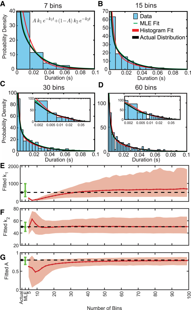
MLE fitting outperforms least-squares fitting of binned data. (A–D) Parameters used for generating data (histograms) according to Eq. 9 are shown in black, whereas the fit to the binned histograms (red) and the MLE fit (green), which is independent of binning, are plotted in each graph. The insets in (C) and (D) show the same data and fits with the x axis on a log scale. (E–G) Average fitted value for the two rates and relative amplitudes, as well as the 95% confidence intervals (error bars and shaded area) obtained by 1000 rounds of simulations. The values used to generate the simulated data are shown by the black dot and black dashed line. To see this figure in color, go online.

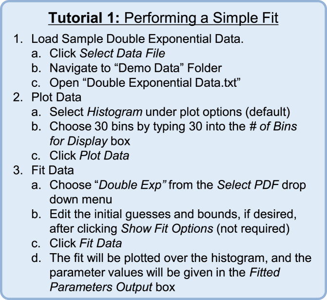
Least-squares fitting of Eq. 9 to histograms containing 7–60 bins created from the simulated data set show that the number of bins has a considerable effect on the values of estimated model parameters (Fig. 1). Plots of best-fit parameters as a function of the number of bins show that the rate (k₁) and amplitude (A) of the fast phase are vastly underestimated when the number of bins is small (<15 bins; Fig. 1, E and G), as the information about this rate is lost by grouping nearly all the fast events into one or two bins (Fig. 1, A and B). For the slower rate (k₂), increasing the number of bins decreases the precision of the determined parameter (Fig. 1 F), which is due to increased stochastic variability in the number of observations in each bin (Fig. 1, C and D). Least-squares fitting of histograms typically overestimates the fast phase (Fig. 1 E). When MEMLET fits the same PDF to the data, it accurately resolves both the fast and slow phases as well as their relative amplitudes with smaller confidence intervals (Fig. 1, E–G, green bar). A tutorial demonstrating how to use MEMLET to perform this type of fit is given in Fig. 2.

Figure 2.

Tutorial 1: Performing a Simple Fit. To see this figure in color, go online.

Fitting of data sets limited by experimental conditions

Data acquisition in most experiments is limited by a t_min, which can be an instrument dead time or minimum signal threshold. For example, in fluorescence imaging experiments, the shortest time a molecular state can be observed will be set by the frame rate of the camera (12, 13, 14), whereas the dead time in optical trapping experiments is often limited by the frequency response of the intrinsic thermal noise of the system (4, 15). If the magnitudes of the events of interest are on the same order as t_min, there may be a significant perturbation on the values of the fitted parameters if the effects of t_min are not considered (4).

Such effects of a t_min in the form of an instrument dead time are demonstrated in Fig. 3, where we simulated a 1000-point data set representing the duration of time that molecules remain in state A until they transition to state B (Eq. 10) at a rate of 50 s⁻¹.

$$\text{A}\stackrel{\text{k}=50{\text{s}}^{-1}}{\to }\text{B}.$$ (10)

The lifetime of the population of A is described by a single-exponential distribution (Fig. 3 A, blue). In the absence of an instrumental dead time, the transition rate can be determined from the simulated data by calculating the inverse of the mean of the durations.

Figure 3.

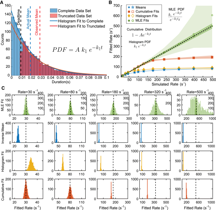
Effect of instrument dead time on determination of the best-fit parameters for different fitting procedures. (A) A simulated single-exponential data set shown as histograms for the complete data set (blue) and the data set subjected to t_min = 10 ms (red). (B) Rates obtained from single exponential fits plotted versus the actual rates of the simulated data, with t_min = 10 ms imposed on the data set. Shown are the rates obtained using the inverse mean method (blue), histogram fits (yellow), cumulative distribution fits (red), and MLE method (green) with the PDFs used for fitting specified for each method. Five hundred rounds of fitting unique simulated data sets yields 90% confidence intervals for each method (shaded areas). The dark shaded areas and closed symbols show how each method performs when the number of points is held constant at 1000 data points, whereas the light-shaded areas and open symbols describe the fit when the number of fitted points is reduced as the rate increases due to t_min. The difference between light and dark is most obvious for the MLE, whereas for the other methods, the dark shaded areas appear as lines and the open and closed symbols are on top of each other. (C) The distribution of fitted rates (histograms) compared to simulated rates (black dashed line) from the 500 simulated data sets subjected to t_min = 10 ms used to generate (B). For the MLE fits, the labels on the left y-axis give the counts for the light areas, whereas the right y-axis labels are the counts for the dark areas. Other methods share the left-axis labels. To see this figure in color, go online.

However, when a t_min threshold is imposed by removing all durations <10 ms, 40% of the events are removed from the analysis (Fig. 3 A, red). Because the events that are missed are the shortest events, the inverse of the mean duration (33 s⁻¹) underestimates the true rate of the process. (Fig. 3 A, dashed red line). A faster rate constant (Fig. 3, B and C, blue) or a longer dead time would result in an even more substantial underestimation of the rate.

Missing events due to a dead time may lead to a reduction in the numbers of events in the shortest-duration bins (Fig. 3 A, red histogram), which can lead to inaccurate rates obtained by least-squares fitting. Fitting the uncorrected single-exponential PDF to the full, binned data set using least-squares fitting yields a rate of 49.5 s⁻¹ (95% confidence interval 48.6–50.4) (Fig. 3 A, blue line), whereas the data subject to the 10 ms dead time yields a rate of 42.5 s⁻¹ (95% confidence interval 39.5–45.6) (Fig. 3 A, red line). Notably, the binned data that are truncated due to t_min can resemble a double-exponential or γ PDF, resulting in the application of an inappropriate kinetic model.

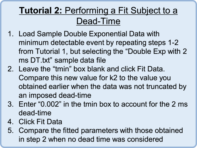
Fig. 3 B shows the effect of a 10 ms dead time on fitted rates obtained via different methods as a function of the rate constant used to simulate the data (k in Eq. 10). As the rate constant is increased, more events are missed from the original 1000 simulated events, until at a rate of 500 s⁻¹ only six events remain. Fitting the standard, uncorrected PDF to histograms using least-squares fitting (Fig. 3, B and C, yellow) will often underestimate the simulated rate when a t_min is present. Adding an additional fitting variable to account for the amplitude when fitting to a cumulative distribution function helps to increase the accuracy of the fit (Fig. 3, B and C, red); however, this method fails at rates >200 s⁻¹ when t_min is more than twice the mean lifetime of the events. Use of MEMLET to fit a dead-time-corrected PDF (as described in Materials and Methods) yields accurate fitting (error <10%), even when t_min is nearly four times larger than the mean lifetime (Fig. 3, B and C, green). Keeping the number of data points constant at 1000, as shown in dark green in Fig. 2, B and C, allows the corrected MLE fit to produce very accurate results with small confidence intervals (Fig. 3 B, dark-shaded regions). Assuming that t_min is known, this MLE method requires fewer free parameters than the cumulative distribution with a free amplitude term. A tutorial demonstrating how to use MEMLET to fit data subject to a dead time is given in Fig. 4.

Figure 4.

Tutorial 2: Performing a Fit Subject to a Dead Time. To see this figure in color, go online.

The effect of t_min on the fit can impact the conclusion of an experiment. For example, the data shown in Fig. 2 could represent fits to a data set produced by an instrument with a 10 ms dead time under various experimental conditions that affect the rate of a studied process. It is clear that as the rate of the reaction increases, the fitted rates plateau for all tested fitting methods except for the corrected MLE fit, leading to a possible misinterpretation of the experimental results. Although other methods exist that can correct for t_min in simple cases such as a when the data are best described by a single-exponential function, MEMLET provides a consistent way to account for t_min across a variety of complex models.

As an aside, which would be a footnote if Biophysical Journal allowed it, for the single-exponential example, a very simple method of estimating the time constant is to subtract t_min from the raw average of the sample durations:

$${\tau }_{\text{est}}=\Sigma {\text{t}}_{\text{i}}/\text{n}-{\text{t}}_{\text{min}},$$ (11)

where n = number of samples. This relationship gives the same values as the green symbols in Fig. 3 B. However, it is only useful for a single-exponential process and does not provide confidence intervals or the other features of MEMLET. Performing such dead-time corrections allows the other methods to perform better than shown in Fig. 3, but MLE will still outperform in challenging circumstances, such as when the number of points is low (Fig. S1 in the Supporting Material).

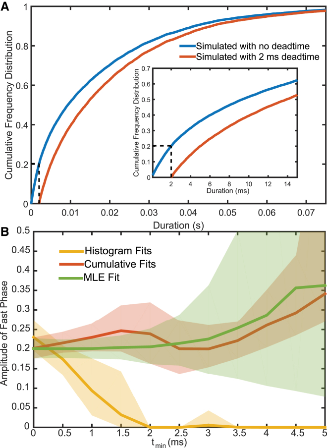
When a process includes transitions to a state via multiple pathways (Eq. 8), it is important to know the relative contribution of each of these pathways, which can be derived from the amplitudes of each exponential component. Estimates of the amplitudes are highly susceptible to distortion when t_min exists. When the simulated data from Fig. 1, which contain two exponential phases, are subjected to a t_min, data originating from the faster phase are more likely to go unobserved (Fig. 5 A). This causes the relative amplitude of the faster phase to be underestimated when using least-squares fitting to a histogram (Fig. 5 B, yellow). Cumulative distributions with an extra free amplitude term yield accurate fits for very small t_min (<0.5 ms, half of the mean lifetime of the fast phase (Fig. 5 B, red)). However, the t_min-corrected MLE fit performed by MEMLET is able to faithfully report the relative amplitudes of each phase to within 10%, even when t_min is the same size as the mean lifetime (2 ms) of the fastest events (Fig. 5 B, green). The ability of MEMLET and other methods to accurately fit double-exponential functions depends greatly on the difference between the two rates of the processes, as shown in Fig. S2.

Figure 5.

Effect of instrument dead time on multicomponent models for different fitting procedures. (A) The empirical cumulative density function (CDF) for the entire simulated data set from Fig. 1 (blue), and the CDF when events <2 ms are removed (red). Vertical dashed lines show the dead time, whereas horizontal dashed lines show the proportion of events missed. The inset shows a zoomed-in view of the same plot. (B) Performance of histogram fits (yellow), cumulative distribution fits (red), and MLE fits (green) in estimating the proportion of fast events as a function of increasing t_min. Shaded areas indicate 95% confidence intervals for the fits estimated from 500 rounds of simulations. To see this figure in color, go online.

Fitting data with multiple dependent variables

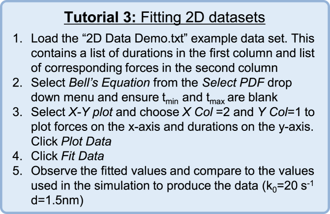
Fitting data consisting of multiple dependent variables can become difficult when the relationship between the variables is not simple. When the residuals of a fit are not normally distributed (e.g., observations of photon counts that follow a Poisson distribution), it is inappropriate to fit the data using least-squares fitting, as the assumptions necessary for least-squares fitting are not met (2). As mentioned, the accuracy of MLE fitting is not dependent on this assumption, and MEMLET can be easily used in cases where two or more dependent variables are present. A tutorial for using MEMLET to fit a data set with two dependent variables is given in Fig. 6.

Figure 6.

Tutorial 3: Fitting 2D Data Sets. To see this figure in color, go online.

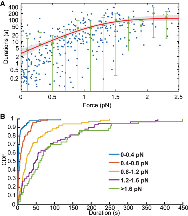
When optical trapping experiments are used to study the force dependence of an association lifetime between two molecules, both the force applied to the molecules and the duration of a single interaction are recorded (4, 16, 17). In Fig. 7, MEMLET has been used to fit a data set from an optical trap experiment studying the durations of attachment between myosin 1b and actin (16). The experiment reveals durations of attachments over a wide distribution of forces (Fig. 7 A). The standard deviations of the grouped data show that at each force, the spread in the durations differs. At forces <1.2 pN, the value of the durations is strongly affected by force, whereas at forces >1.2 pN, there is little change in the mean duration as force increases (Fig. 7 B). This suggests that the overall rate of dissociation, k, is given by the sum of a force-independent rate (k_i) that dominates at high forces and a force-dependent rate (k_F) that dominates at lower forces, as shown by the scheme in Eq. 12 and Eq. 13:

$$\begin{array}{c}\text{Attached}\\ \begin{array}{cc}\begin{array}{cc}{\text{k}}_{\text{F}}\left(\text{F}\right)& \downarrow \end{array}& \begin{array}{cc}\downarrow & {\text{k}}_{\text{i}}\end{array}\end{array}\\ \text{Detached}\end{array},$$ (12)

$$k=k_F+k_i=k_0\times e^{-\frac{F\cdot d}{k_{B}T}}+k_i,$$ (13)

where k₀ is the rate of the force-dependent transition at zero load, F is the force, d is the “distance parameter,” which indicates the sensitivity of rate on force, k_B is Boltzmann’s constant, and T is the temperature. The distribution of attachment durations will be exponentially distributed at this summed rate (k_i + k_F) at each force, but the overall distribution of all attachment durations will not be exponentially distributed, causing the data points to appear very disperse (Fig. 7 A).

Figure 7.

MEMLET can determine nonlinear relationships among multiple dependent variables. (A) Data points representing actomyosin attachment duration data from Laakso et al. (17) (blue), with data grouped by force in 0.5 pN bins with standard deviations (green bars; no binning was used for fitting). The MLE fit (red) using the PDF in Eq. 13 describes the scheme in Eq. 12 with 90% confidence intervals (gray shaded area) determined from 500 rounds of bootstrapping. (B) The calculated CDF of the data in (A) grouped in specified force ranges, showing that the rate of the process is force dependent at low forces (0–1.2 pN), but force independent at higher forces (>1.2 pN), as shown in Eq. 12. To see this figure in color, go online.

MEMLET is capable of fitting this complex model to the data while taking into account an instrument dead time (Fig. 7 A; Table S1). A simulated data set of similar characteristics and the corresponding fit are shown in Fig. S3 and Tables S2 and S3, alongside other possible parameter values, illustrating the program’s ability to accurately fit this type of complex distribution.

Determining the statistical justification of additional fitted parameters

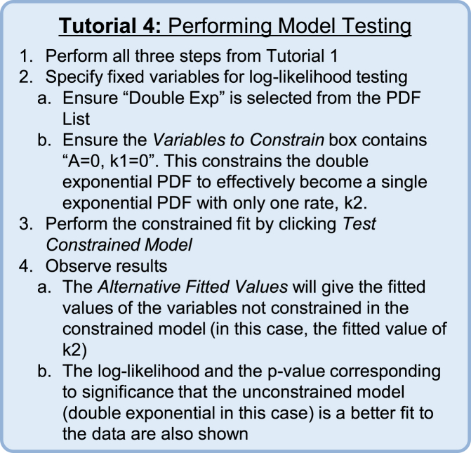
It is often nontrivial to decide which model is the appropriate choice to describe a given data set. The program presented here provides a log-likelihood-based method (described above in Theory: Likelihood Ratio Testing) for quantitatively determining whether a PDF with more free fitting variables fits significantly better than a constrained version of that PDF with fewer free parameters. To demonstrate this functionality in MEMLET, Tutorial 4 (Fig. 8) shows how to determine if adding an additional exponential phase to a single-exponential distribution is statistically justified in a simulated data set. After following the described procedure for statistical testing, MEMLET provides a p-value giving the probability that the model with fewer fitted parameters is a statistically better fit over the more complex model when accounting for the increased number of free parameters (i.e., if p = 0.05, there is 95% confidence that the model with the additional parameters is a statistically better fit). An example of how well this test can discriminate the two phases of a double-exponential distribution as a function of the difference between the two rates is shown in Fig. S2.

Figure 8.

Tutorial 4: Performing Model Testing. To see this figure in color, go online.

This test can be applied to the data presented in Fig. 7 to determine whether the observed data require a force-dependent term for significance or can be adequately described by a simpler model function. For the data in Fig. 7, it was previously determined using MLE-based methods that the data are well described by a process that includes a force-dependent process as well as a parallel, force-independent process, as shown in Eq. 12 (16). A PDF describing a process with both a force-dependent and a force-independent process can be input as a custom PDF into the fitting program, and the log-likelihood testing function can be used to determine that this indeed yields a better fit to the data than either a single force-dependent or a single force-independent process (p < 10⁻⁶; see Table S1), and that the free parameters, k_i, k₀, and d, are all statistically justified.

Global fitting

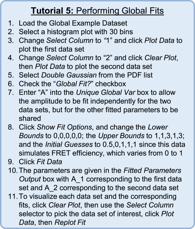
In some cases, multiple data sets might be described by distributions that share some, but not all, of the same parameter values. For example, by changing the value of an independent variable across experiments, such as the concentration of a solute (ions, nucleotide, etc.), one rate of a multirate process may be changed without affecting the other rates present. MEMLET is capable of using multiple data sets acquired under various conditions to fit a given model, letting the user specify which fitting parameters are shared between the data sets and which vary in different experimental conditions, as demonstrated by the global fitting tutorial (Fig. 9).

Figure 9.

Tutorial 5: Performing Global Fits. To see this figure in color, go online.

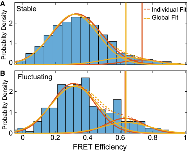
As an example, we apply this procedure to single-molecule Förster resonance energy transfer (FRET) data from Chen et al. (18), shown in Fig. 10, where the FRET value signals the distance between a fluorophore on a ribosomal subunit (L11) and a fluorophore on a tRNA during the translation of a peptide sequence (18).

Figure 10.

Global Fitting in MEMLET improves precision of fitting multiple data sets. Fitting of FRET efficiency data from Fig. 3 D of Chen et al. (18) shows two populations of FRET efficiencies in two data sets, referred to as (A) stable and (B) fluctuating. Each data set was fit individually with a double-Gaussian PDF (dashed red lines; solid lines show individual Gaussian components). The global fit (yellow) constrained the position and width of both Gaussian components while allowing the relative amplitudes to vary between the data sets. Vertical lines show the fitted position of the high FRET peak for the individual (red) and global (yellow) fits. To see this figure in color, go online.

The ribosomes were in a pre-translocation complex waiting for the translocase, elongation factor G, to bind. As evidenced from time courses of the FRET efficiency (Fig. 3, A and B, in (18)), some of the ribosomes fluctuated between two pre-translocation structures, termed “classic” and “hybrid,” whereas other ribosomes stably occupied either the classic or hybrid pre-translocation state. For both stable and fluctuating ribosomes, the distributions of FRET efficiencies between two fluorophores were best described by the sum of two Gaussian distributions, the two components being justified by the log-likelihood-ratio test described above (p-value of 2 × 10⁻¹² and 0.00319 for the stable and fluctuating data sets, respectively). Are the mean positions of the FRET peaks the same in both data sets? When fitting the data sets independently (Fig. 10, red), the apparent position of the higher FRET peak differs between the stable and fluctuating ribosomes. This might be due to the high FRET peak containing a small percentage of events in the stable data (∼10%), thereby biasing or reducing the precision of the fitted peak. The global fitting feature of MEMLET allows the peak positions and widths to be specified as shared parameters, with only the relative amplitude of each peak being unique between the data sets. This global model (Fig. 10, yellow) yields a good fit to the data, and it allows the relative amplitudes of the two FRET values to be accurately compared between the stable and fluctuating ribosome classes. The log-likelihood-ratio test shows that using the individual fit parameters for each data set is not statistically justified (Table S4). A simulated data set with similar parameters (Fig. S4; Table S5) demonstrates that the global fitting implementation is capable of increasing the accuracy and precision of fitting in such cases when the number of points in a particular data set is small. In such situations, where multiple-component distributions are used, users are encouraged to perform similar simulations that emulate their experimental data to ensure that their fitted parameters can be reliably determined.

Conclusions

The provided program offers an easy-to-use and accessible method for researchers with a wide range of computational expertise to utilize MLE to fit their data. In addition to a simple graphical user interface, many of the program’s functionalities are accessible and can be enhanced by editing and writing further scripts in MATLAB. The included documentation makes it easy to fit the data to predefined PDFs, utilize custom PDFs, estimate uncertainties using bootstrapping, and test whether adding additional parameters to a model is statistically justified. By easily allowing users to automatically renormalize a PDF to account for the size of their minimum or maximum detectable event (t_min or t_max), the accuracy of fitting is greatly improved. For more complex data sets, the ability to perform global fitting and utilize multidimensional data enables thorough analysis. The program runs in the MATLAB programming environment, and is also available as a stand-alone application that only requires the freely available MATLAB Runtime Program. Both versions of the program, as well as the associated help files, are available on GitHub for download.

Program availability

The program is available on the GitHub repository hosting service and includes the program files, stand-alone installer, documentation, and demo data at: http://dx.doi.org/10.5281/zenodo.55586

An accompanying web site can be found at http://michaelswoody.github.io/MEMLET/

Author Contributions

M.S.W. wrote the program code and carried out the simulations and analysis. All of the authors contributed to program and algorithm design. M.S.W., Y.E.G., and E.M.O. wrote the manuscript.

Editor: Stefan Diez.

References

- 1.Fisher R.A. On the mathematical foundations of theoretical statistics. Philos. Trans. A Math. Phys. Eng. Sci. 1922;222:309–368. doi: 10.1098/rsta.2014.0252. [DOI] [PMC free article] [PubMed] [Google Scholar]
- 2.Bevington P.R., Robinson D.K. McGraw-Hill; New York: 2003. Data Reduction and Error Analysis for the Physical Sciences. [Google Scholar]
- 3.Myung I.J. Tutorial on maximum likelihood estimation. J. Math. Psychol. 2003;47:90–100. [Google Scholar]
- 4.Greenberg M.J., Shuman H., Ostap E.M. Inherent force-dependent properties of β-cardiac myosin contribute to the force-velocity relationship of cardiac muscle. Biophys. J. 2014;107:L41–L44. doi: 10.1016/j.bpj.2014.11.005. [DOI] [PMC free article] [PubMed] [Google Scholar]
- 5.Hines K.E. A primer on Bayesian inference for biophysical systems. Biophys. J. 2015;108:2103–2113. doi: 10.1016/j.bpj.2015.03.042. [DOI] [PMC free article] [PubMed] [Google Scholar]
- 6.Wilks S.S. The large-sample distribution of the likelihood ratio for testing composite hypotheses. Ann. Math. Stat. 1938;9:60–62. [Google Scholar]
- 7.Press W.H. Cambridge University Press; Cambridge, United Kingdom: 2002. Numerical Recipes in C++: The Art of Scientific Computing. [Google Scholar]
- 8.Efron B. Society for Industrial and Applied Mathematics; Philadelphia, PA: 1982. The Jackknife, the Bootstrap and Other Resampling Plans. [Google Scholar]
- 9.Aldrich J. R. A. Fisher and the making of maximum likelihood 1912–1922. Stat. Sci. 1997;12:162–176. [Google Scholar]
- 10.Ingber L. Adaptive simulated annealing (ASA): lessons learned. Control Cybern. 1996;25:33–54. [Google Scholar]
- 11.Ross S.M. Harcourt/Academic Press; Cambridge, MA: 2000. Introduction to Probability Models. [Google Scholar]
- 12.Holden S.J., Uphoff S., Kapanidis A.N. Defining the limits of single-molecule FRET resolution in TIRF microscopy. Biophys. J. 2010;99:3102–3111. doi: 10.1016/j.bpj.2010.09.005. [DOI] [PMC free article] [PubMed] [Google Scholar]
- 13.Nirschl J.J., Magiera M.M., Holzbaur E.L.F. α-Tubulin tyrosination and CLIP-170 phosphorylation regulate the initiation of dynein-driven transport in neurons. Cell Reports. 2016;14:2637–2652. doi: 10.1016/j.celrep.2016.02.046. [DOI] [PMC free article] [PubMed] [Google Scholar]
- 14.Liu W., Chen C., Cooperman B.S. EF-Tu dynamics during pre-translocation complex formation: EF-Tu·GDP exits the ribosome via two different pathways. Nucleic Acids Res. 2015;43:9519–9528. doi: 10.1093/nar/gkv856. [DOI] [PMC free article] [PubMed] [Google Scholar]
- 15.Capitanio M., Canepari M., Pavone F.S. Ultrafast force-clamp spectroscopy of single molecules reveals load dependence of myosin working stroke. Nat. Methods. 2012;9:1013–1019. doi: 10.1038/nmeth.2152. [DOI] [PubMed] [Google Scholar]
- 16.Laakso J.M., Lewis J.H., Ostap E.M. Control of myosin-I force sensing by alternative splicing. Proc. Natl. Acad. Sci. USA. 2010;107:698–702. doi: 10.1073/pnas.0911426107. [DOI] [PMC free article] [PubMed] [Google Scholar]
- 17.Laakso J.M., Lewis J.H., Ostap E.M. Myosin I can act as a molecular force sensor. Science. 2008;321:133–136. doi: 10.1126/science.1159419. [DOI] [PMC free article] [PubMed] [Google Scholar]
- 18.Chen C., Stevens B., Goldman Y.E. Allosteric vs. spontaneous exit-site (E-site) tRNA dissociation early in protein synthesis. Proc. Natl. Acad. Sci. USA. 2011;108:16980–16985. doi: 10.1073/pnas.1106999108. [DOI] [PMC free article] [PubMed] [Google Scholar]
Associated Data
This section collects any data citations, data availability statements, or supplementary materials included in this article.