Automated identification of abnormal respiratory ciliary motion in nasal biopsies

Abstract

Motile cilia lining the nasal and bronchial passages beat synchronously to clear mucus and foreign matter from the respiratory tract. This mucociliary defense mechanism is essential for pulmonary health, because respiratory ciliary motion defects, such as those in patients with primary ciliary dyskinesia (PCD) or congenital heart disease, can cause severe sinopulmonary disease necessitating organ transplant. The visual examination of nasal or bronchial biopsies is critical for the diagnosis of ciliary motion defects, but these analyses are highly subjective and error-prone. Although ciliary beat frequency can be computed, this metric cannot sensitively characterize ciliary motion defects. Furthermore, PCD can present without any ultrastructural defects, limiting the use of other detection methods, such as electron microscopy. Therefore, an unbiased, computational method for analyzing ciliary motion is clinically compelling. We present a computational pipeline using algorithms from computer vision and machine learning to decompose ciliary motion into quantitative elemental components. Using this framework, we constructed digital signatures for ciliary motion recognition and quantified specific properties of the ciliary motion that allowed high-throughput classification of ciliary motion as normal or abnormal. We achieved >90% classification accuracy in two independent data cohorts composed of patients with congenital heart disease, PCD, or heterotaxy, as well as healthy controls. Clinicians without specialized knowledge in machine learning or computer vision can operate this pipeline as a “black box” toolkit to evaluate ciliary motion.

INTRODUCTION

Cilia are microtubule-based hair-like projections of the cell; in humans, they are found on nearly every cell of the body. Cilia can be motile or immotile. Diseases known as ciliopathies where cilia function is disrupted can result in a wide spectrum of diseases. In primary ciliary dyskinesia (PCD), airway cilia that normally beat in synchrony to mediate mucus clearance can exhibit dyskinetic motion or become immotile, resulting in severe sinopulmonary disease (1–4). Because motile cilia are also required for left-right patterning, PCD patients can exhibit mirror symmetric organ placement, such as in Kartagener’s syndrome, or randomized left-right organ placement, such as in heterotaxy. Patients with congenital heart disease and heterotaxy exhibit a high prevalence of ciliary motion (CM) defects similar to those seen with PCD (5). CM defects have been associated with increased respiratory complications and poor postsurgical outcomes (5–8). Similar findings were observed in patients with a variety of other congenital heart diseases, including transposition of the great arteries (TGA) (9, 10). Early diagnosis of CM abnormalities may provide the clinician with opportunities to institute prophylactic respiratory therapies that could improve long-term outcomes in patients.

Current methods for assessing CM rely on a combination of tools comprising a “diagnostic ensemble.” Electron microscopy, considered one of the most reliable methods of the ensemble, cannot identify PCD patients who present without ultrastructural defects (11). Video-microscopy of nasal brush biopsies can be used to compute ciliary beat frequency (CBF) (12–15), but this metric has low sensitivity to detect abnormal CM, because it does not capture the broad distribution of frequencies present in ciliary biopsies (3, 11, 16–19). Currently, the most robust method for identifying abnormal CM entails visual examination of the videomicroscope nasal brush biopsies by expert reviewers for ciliary beat abnormalities. This is often used clinically to identify patients with CM abnormalities. However, the reliance on visual evaluations by expert reviewers makes these assessments time-consuming, highly subjective, and error-prone (17, 20). Additionally, manual evaluations are not amenable to cross-institutional comparisons.

To overcome these deficiencies, we developed an objective, computational method for quantitative assessment of CM. In this computational framework, we consider CM as an instance of dynamic texture (21, 22). Dynamic textures are modeled as rhythmic motions of particles subjected to stochastic noise (23–26). Examples of dynamic textures include familiar motion patterns such as flickering flames, rippling water, and grass in the wind, each with a small amount of stochastic behavior altering an otherwise regular visual pattern. Dynamic texture analysis has been shown to be an effective analysis method in other biomedical contexts, such as localizing cardiac tissue in three-dimensional time-lapse heart renderings (27) and the quantitation of thrombus formations in time-lapse microscopy (28). CM is well described as a dynamic texture, as it consists of rhythmic behavior subject to stochastic noise that collectively determine the beat pattern. Here, we present a computational pipeline that uses dynamic texture analyses to decompose the CM observed in high-speed digital videos into idealized, or elemental, components (26, 29).

Two distinct methods were tested for generating “digital signatures,” or quantitative descriptions of the CM, from the elemental components. Both methods obtained robust results on two independent patient data sets of differing quality, recapitulating the expert assessment of ciliary beat pattern to a high degree of accuracy. Our pipeline can be used as a “black box” tool by clinicians and researchers without specialized knowledge in machine learning or computer vision, rendering CM predictions in an objective and quantitative fashion and eliminating reviewer subjectivity. Although this study focuses on identifying abnormal CM in patients with PCD and congenital heart disease, this framework could be used to analyze CM across a broad spectrum of ciliopathies and related disorders.

RESULTS

Decomposing CM into elemental components

A critical hurdle in CM evaluation is accounting for and capturing a diversity of motion phenotypes. A single nasal brush biopsy often contains a spectrum of beat frequencies and motile cilia behaviors. Consequently, a single numerical value, such as CBF, cannot encapsulate the heterogeneity of CM phenotypes (Fig. 1A and movies S1 to S5). CM heterogeneity can arise from multiple sources: as an inherent property of the cilia in the sample, technical artifacts (for example, overlapping cilia), background particulate obstructing proper view of the cilia, and video capture artifacts (for example, changes in the plane of focus and translational motion of the sample) (movies S6 and S7).

Fig. 1. Properties of CM.

(A) Schematic (hand-drawn) diagrams of CM subtypes to aid clinical diagnosis. (B) Stacked frames indicate still frames of the video of the CM biopsy, and the black box indicates the ROI selected by the clinician. (C) Yellow arrows on the images from (B) indicate direction and magnitude of optical flow for a small region of the video for each pair of frames. (D) Changes in the optical flow are used to compute the elemental components. Red arrows, optical flow at frame t; green arrows, optical flow at frame t + 1; blue arrows, optical flow at frame t + 2. (E) Elemental components of rotation (top left), deformation (top right, bottom right), and divergence (bottom left; excluded from analysis), shown here in a template form. Deformation is a vectorial quantity requiring two templates for measurement.

We modeled CM heterogeneity by first computing the optical flow in user-specified regions of interest (ROIs) in the digital videos (Fig. 1B). Conceptually, optical flow (29) models the apparent motion between two frames as a vector field, indicating the direction and magnitude of apparent motion at each pixel position in the ROI (Fig. 1C). Optical flow does not explicitly track particles but rather provides an estimate of the local motion, or flow, at each pixel from frame to frame. We provide a detailed overview and derivation of optical flow in the Supplementary Materials and Methods.

Using the spatial and temporal derivatives of the optical flow (Fig. 1D), we computed elemental components of the CM, specifically instantaneous rotation (curl) and deformation (biaxial shear) (Fig. 1E) (30, 31). These elemental components can be conceptualized as videos, each of which has the same height, width, and number of frames as the original ciliary biopsy videos. However, instead of grayscale pixel intensities, the values of the elemental components are used in each pixel position. Deformation, like optical flow, is a vector quantity with x and y components at each pixel position (Fig. 1E, right column) and unit pixels/s, whereas rotation is a scalar quantity at each pixel position and has units radians/s (21).

In computing elemental components at each pixel, we aim to uncover fundamental variations in the temporal evolution and spatial distribution of the elemental components as a means to differentiate normal from abnormal CM. Figure 2 compares the CM waveforms at three pixel locations in normal and abnormal CM in terms of grayscale pixel intensities, rotation, and deformation amplitude. Pixel positions in Fig. 2A were chosen to compare waveforms at the proximal (blue) and distal (red) regions of cilia, as well as background motion of the biopsy suspension medium (black). Like pixel intensities (Fig. 2B), elemental components exhibit periodic temporal behavior, particularly at the distal regions of the cilia (red). Rotation (Fig. 2C) and deformation (Fig. 2D) computed for healthy CM showed strong periodic behavior and large magnitudes. By contrast, the rotation and deformation in abnormal cilia showed erratic, weakly periodic behavior in addition to reduced magnitudes.

Fig. 2. Digital representations of pixels in ciliary biopsy videos.

(A) Single frame of a video of normal and abnormal CM with three pixels identified: blue (proximal to cell wall), red (distal from cell wall), and black (background). See movies S1 to S9 for examples of normal and abnormal CM. (B) Time series of gray-level pixel intensities over 100 frames at each of the three respective pixel locations in (A). (C) Time series of rotation over 100 frames at each of the respective pixel locations in (A). (D) Time series of deformation amplitude over 100 frames at each of the respective pixel locations in (A). a.u., arbitrary units.

There are at least two technical advantages of using elemental components instead of grayscale pixel intensities in our analyses. One is the ability to directly compare these quantities between video samples without regard to lighting conditions or microscope settings, because relative brightness difference between two videos does not inherently signify a difference in CM. Second, elemental components are orientation-invariant; other methods for generating quantitative descriptions of images rely on specific orientations of the objects of interest (Supplementary Materials and Methods) (24–26). In particular, we used principal components analysis (PCA) to reduce the dimensionality of the elemental components. PCA realigns the axes of the data in the directions of maximal variance. Because elemental components are computed from the magnitudes of optical flow derivatives, the relative orientation of structures in the videos is irrelevant to elemental component computations. In practical terms, this allows videos of cilia to be analyzed in tandem regardless of the perspective of the cilia relative to the camera.

From elemental components to digital signatures

Autoregressive models

Our first method for computing digital signatures from the elemental components involved the use of autoregressive (AR) processes. AR models are linear dynamics systems that are useful for representing periodic signals, and are among the state-of-the-art dynamic texture analysis methods (22, 23, 27, 28). Although linear models can be limited in their ability to capture complex behaviors, the high capture speed of most ciliary biopsy videos (200 Hz) guarantees that linear transformations will be sufficient to model the motion between successive frames (fig. S1). We used the formulation of AR processes as defined in Eq. 1 (23, 32). Briefly, this formulation embeds the CM in a low-dimensional space using PCA to capture as much of the variance in the data in as few dimensions as possible. The first five principal components of the rotation data captured more than 90% of the variance (Fig. 3A). By fitting the rotation and deformation time series to linear equations (Eq. 2 and Fig. 3B), we used the resulting coefficients of the equations—the quantitative basis for CM in the PCA space—as the digital signatures of the CM.

Fig. 3. CM AR representations.

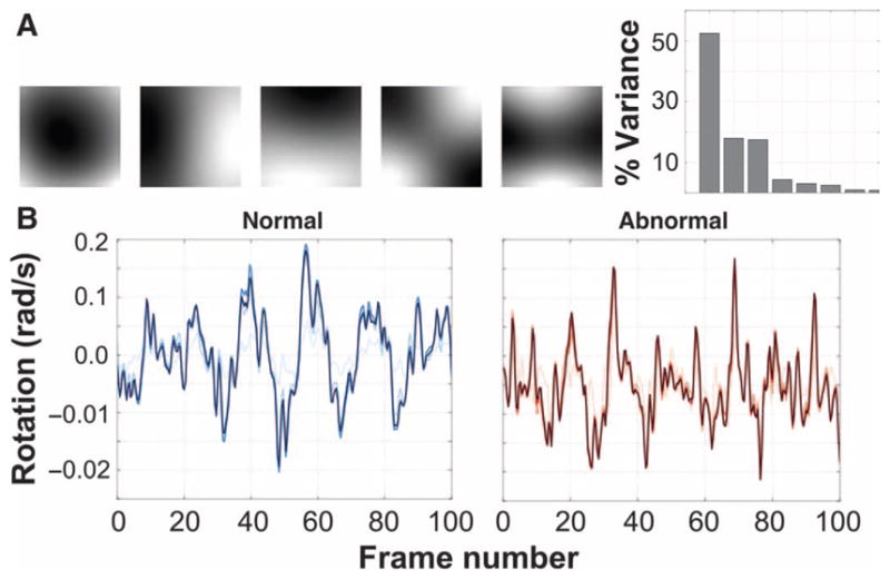
(A) Top five principal components of CHP rotation data and the percentage of the overall variance in the CM data explained by each component. The top q principal components are used to compute the AR motion parameters. (B) One-dimensional rotation signal from a single pixel of normal (left) and abnormal (right) CM as the original signal (darkest blue/red) is reconstructed using an increasing number of principal components. Darker lines indicate larger q (shown: q = 2, q = 5, and q = 10).

Magnitude and frequency histograms

Our second method for computing digital signatures involved histograms to represent the distributions of elemental components present in CM samples. For each CM sample, we computed four histograms to represent the distributions of four CM quantities: rotation magnitude, deformation magnitude, rotation frequency, and deformation frequency. The magnitude histograms (Fig. 4A) were built by placing all computed rotation and deformation values into respective histograms. The frequency histograms (Fig. 4B) were computed by transforming the time-series rotation and deformation data into the frequency domain using a fast Fourier transform. Specifically, we computed a spectrogram (33), or a sliding average of frequency spectra. We computed the dominant frequency present at each pixel position (analogous to computing CBF from pixel intensity variations) (fig. S2) and placed the dominant frequencies from rotation and deformation into respective histograms. These four histograms collectively comprised the digital signature of the CM for the histogram method. Using the histograms, we could visually observe any differences in the overall distributions of rotation and deformation between normal and abnormal CM.

Fig. 4. CM histogram representations and results.

(A) Time domain histograms of ciliary rotation and deformation magnitudes from normal (blue) and abnormal (red) CM. The time series in Fig. 2 was projected onto the vertical axis and normalized. (B) Frequency domain histograms of ciliary rotation and deformation time series from normal and abnormal CM. A fast Fourier transform was used on the rotation and deformation time series, the dominant frequency at each pixel was computed from the Fourier response, and histograms of these frequencies for rotation and deformation were plotted.

Using digital signatures to classify CM

We used two patient CM data cohorts (Table 1 and fig. S3). The first cohort consisted of videos of CM biopsies from 49 individuals (27 healthy controls, 5 PCD controls, and 17 TGA patients with abnormal CM) recruited from Children’s Hospital of Pittsburgh (CHP cohort). The second cohort consisted of videos from 31 subjects (27 patients with heterotaxy—10 abnormal CM, 17 normal CM—and 4 PCD controls) recruited from the Children’s National Medical Center (CNMC cohort) reported in (6). With these two cohorts, we evaluated the performance of our pipeline by using the manual beat pattern calls made by blinded experts as ground truth, and compared the CM predictions made by the pipeline to the ground truth. We also compared our pipeline to baseline automated methods using CBF and pixel intensities (Table 2).

Table 1. Description and breakdown of data sets.

Both data cohorts consisted of a mix of patients for whom their CM was assessed manually as either normal or abnormal; these assessments were used as ground truth for validating our framework. Multiple video samples were generated for each patient, and from these videos, multiple ROIs were selected for analysis. CHD, congenital heart disease.

Diagnosis	Individuals	Videos	ROIs
Children’s Hospital of Pittsburgh
Healthy controls	27	76	114
PCD controls	5	38	96
CHD/TGA with abnormal CM	17	56	121
Total	49	170	331
Children’s National Medical Center
PCD controls	4	25	58
Heterotaxy with normal CM	17	65	139
Heterotaxy with abnormal CM	10	31	65
Total	31	121	262

Table 2. Classification accuracy, sensitivity, and specificity on both data cohorts, with each proposed method.

We compare the performance of our methods to two baseline methods: classification using the histogram method on the gray-level pixel intensities in lieu of computing optical flow, and using CBF.

Method	Data set	Accuracy (%)	Sensitivity (%)	Specificity (%)
Proposed methods
Histogram	CHP	93.88	95.24	92.86
AR (rotation)	CHP	88.64	80.00	95.83
AR (deformation)	CHP	86.36	76.19	95.65
Histogram	CNMC	86.67	91.67	83.33
AR (rotation)	CNMC	83.33	83.33	83.33
AR (deformation)	CNMC	70.00	59.09	100.00
Baseline methods
Histogram (intensities)	CHP	72.73	63.16	80.00
CBF	CHP	52.27	35.00	58.33

Having constructed digital signatures from both data cohorts and established CM ground truth (see Materials and Methods), the final step in our pipeline involved supervised classification (fig. S4). There are many supervised algorithms available; we used a support vector machine (SVM) because SVMs are known to perform well with high-dimensional data. Functionally, each ROI could be considered a point in high-dimensional space; thus, any linear classifier (including SVMs) will attempt to find a plane in that space that most accurately separates the normal instances from the abnormal ones (see Materials and Methods for specific data structure layouts). The hyperparameters used in training the SVM, as well as constructing the digital signatures, can be found in table S1.

We performed 10-fold cross-validation, averaged over 100 randomized iterations, on both cohorts independently. Each ROI was a single data point; therefore, to provide CM predictions at the patient level, a consensus classification step was used, in which the CM predictions for each ROI influenced the final CM prediction for the patient. We report the result of consensus classification, averaged over all 100 randomized iterations, as the final accuracy for each method (fig. S4). For the first (CHP) cohort, classification using the AR method achieved an optimal accuracy of 88.6% with rotation and 86.4% with deformation, and the histogram method reached 93.8% accuracy. For the second (CNMC) cohort, the AR method yielded an accuracy of 83.3% using rotation and 70.0% with deformation, and the histogram method obtained 86.7% accuracy.

PCD was the most accurately identified motion abnormality. In the CHP cohort, it was correctly classified as abnormal 93.5% of the time; in the CNMC cohort, it was correctly classified 100% of the time. These results, as well as their sensitivity, specificity, and comparison to the baseline methods, can be found in Table 2. CBF was used as one of the baseline methods because of its typical use in conjunction with electron microscopy and manual visual assessment in identifying CM. The other baseline consisted of adapting our histogram method for use with raw pixel intensities. In these cases, classification using our proposed digital signatures far outperformed the baseline methods.

Examples of misclassifications by our pipeline are shown in movies S8 and S9. In movie S8, the dyskinetic motion exhibits a larger freedom of movement than was typical for abnormal CM, resulting in our framework misclassifying this instance as healthy. In movie S9, while depicting normal motion, the top-down perspective (as opposed to the side profile, which constituted the majority of our data) limited the degree of observable motion, resulting in digital signatures more characteristic of abnormal motion.

Quantitative distinctions between normal and abnormal CM

The magnitude histograms depicted a broad distribution of rotation and deformation values for normal motion relative to the narrower distributions of rotation and deformation for abnormal motion (Fig. 4A). The frequency histograms depicted a clear dominant frequency in normal CM, contrasted again with abnormal CM in which the power was spread over many frequencies (Fig. 4B). Qualitatively, we can characterize normal CM as having a relatively uniform beat frequency, but which rotates or deforms with a relatively wide variance, suggesting much greater freedom of movement than abnormal CM.

We found a similar effect from examining the AR coefficients of normal cilia compared to those from abnormal CM. As visualized in the PCA space, the normal CM showed more freedom of movement than did the abnormal CM (Fig. 5A). Although there was a large overlap between normal and abnormal CM in one dimension (Fig. 5B, left), two or three dimensions (Fig. 5B, middle and right, respectively) depicted a noticeable separation in the motion patterns between normal and abnormal CM, where the motion of abnormal cilia was considerably more restricted by comparison.

Fig. 5. CM AR model results.

(A) CM is visualized using the first three dimensions of the subspace of the AR model for normal and abnormal CM. This motion is governed by the AR coefficients. Passage of time is indicated by hue, darkening with each discrete time increment. (B) Histograms show the distributions of values taken by normal and abnormal AR motion in each of the first three PCA dimensions.

Confidence in identifying PCD patients

We note that among both data cohorts, the PCD controls were consistently identified as exhibiting abnormal CM by both methods; these were among the CM instances our pipeline classified with the greatest confidence. This confidence was determined by averaging the individual patient classification accuracies over the cross-validation iterations. The histogram method, especially in the CHP cohort, was confident in nearly all the predictions it made. This is shown in fig. S5, where the accuracy for each patient tended to be either 0 or 100%, with few in between, irrespective of the number of ROIs per patient. The AR method (fig. S5) tended to be more sensitive to training sets used in the cross-validation iterations, because we observed very few perfect patient-level average classification accuracies.

DISCUSSION

Here, we addressed the unmet clinical need of quantitatively representing CM with two approaches: AR models and histograms. Both methods for computing digital signatures resulted in CM identification accuracy that rivaled manual expert assessment, correctly classifying abnormal cilia in nasal biopsies from more than 90% of all patients and nearly 100% of patients with PCD. Considering the CM as dynamic textures permitted the use of sophisticated dynamic texture analysis techniques, such as AR models, and more intuitive methods, such as histograms.

Of the two elemental components used in this study, rotation most accurately differentiated normal from abnormal CM. Despite the subjectivity in manual identification of ciliary beat pattern, clinical studies consistently describe abnormal motion as having reduced beat amplitude, stiff beat pattern, failure to bend along the length of the ciliary shaft, static cilia, or a flicking or twitching motion (16, 17). Rotation in particular is affected by the stiffness that is often observed in abnormal CM, providing a conceptual link between CM phenotype and the resulting digital signatures.

The few misclassifications made by our pipeline could be attributed to either poor sample and video quality (movies S6 and S7) or possible error in the determination of ground truth CM by our expert panel. These artifacts, when converted to digital signatures, closely mimicked those of normal CM. This effect is particularly prevalent in the CNMC data set where the data were noisier, explaining the lower specificity. Regarding possible ground truth error, there were five CNMC patients consistently misclassified but whose data contained no noticeable recording artifacts. Closer inspection revealed that these patients were potentially assessed incorrectly by the expert panel. For all five patients, the majority vote in establishing ground truth CM was not unanimous, underscoring the primary motivation for developing this pipeline: establishing a quantitative ground truth and eliminating subjective, manual reviewer assessment of CM.

The consensus classification step in the pipeline (fig. S4) enhanced robustness to noise. By generating multiple digital signatures for each patient, classifying them independently, and merging their results into a single CM prediction for the patient, the effects of noisy data on automated CM recognition could be minimized. We found that, beyond a minimum number of roughly three ROIs per patient, the quality of the ROI selection (and, by proxy, the video samples) was more important than the quantity of ROIs. This reliance on manual ROI selection by experts is one limitation in our approach. Future work that includes an intelligent patch-sampling strategy will help begin the process of fully automating the pipeline.

We envision the computational pipeline described here to be deployed in a clinical setting to objectively and quantitatively identify CM defects, enabling multicenter trials to effectively compare findings from ciliary biopsies. This pipeline is applicable to any environment in which CM assessment plays a role, including common airways diseases, cystic fibrosis, or asthma (2, 5–7, 9, 10, 34). Our pipeline will be made accessible to researchers across the world as a web service. To this end, we have designed a prototype web interface for uploading videos and annotating them with ROIs (fig. S6). Using this web interface, it will be possible to pursue a multicenter international “computational ciliary motion assessment” (CCMA) trial. This will establish and validate a standardized protocol for automated CM defect identification in PCD patients and patients with other ciliopathies or respiratory diseases. In the future, CCMA may serve as a rapid first tier screen to identify at-risk patients who would warrant further testing using other modalities (genetic testing, nasal nitric oxide measurement, and ultrastructural analysis by electron microscopy or immunofluorescence imaging) to establish a clinical diagnosis.

Overall, our computational approach improves on the current methods for ciliary beat pattern analysis by using computer vision techniques to replicate expert CM assessment to a high level of accuracy. This approach demonstrates the efficacy of analyzing elemental components for differentiating normal and abnormal CM and eliminating reviewer subjectivity that is inherent even to expert analysis.

MATERIALS AND METHODS

Study design

The overall objective of this study was to develop a computational CM analysis pipeline, which achieved parity with manual expert beat pattern assessment of CM. From CHP, 49 patients were recruited with TGA. Additionally, 27 healthy subjects were recruited to serve as controls. Informed consent was obtained from adult subjects or parents/ guardians of children, with assent obtained from children over 7 years of age. In addition, we recruited five PCD patients to serve as abnormal controls. The resulting corpus formed the first data cohort (CHP), depicting biopsies from 49 individuals (27 healthy controls, 5 PCD controls, and 17 TGA patients). The second cohort consisted of nasal biopsy videos from 31 subjects from CNMC that have been described previously (6). Twenty-seven subjects were patients with heterotaxy: 17 had normal CM and 10 had abnormal CM, as evaluated by a blinded panel of investigators in an identical manner to the CHP cohort. Four additional subjects were included as PCD controls (fig. S3). The video samples were examined by the authors of this study, and data from numerous subjects were discarded on the grounds of spurious camera motion, variable lighting conditions, poor focus, and other recording artifacts. All study protocols were approved by the University of Pittsburgh Institutional Review Board. This study was not blinded.

Data acquisition

Nasal epithelial tissue was collected by curettage of the inferior nasal turbinate under direct visualization using an appropriately sized nasal speculum using Rhino-probe (Arlington Scientific). Nasal brushings and tracheal biopsies have been shown to provide tissue of comparable quality and similar pathology with increased sensitivity over nasal biopsies (35–37). Three passages were made, and the collected tissue was resuspended in L-15 medium (Invitrogen) for immediate video-microscopy using a Leica inverted microscope with a 100× oil objective and differential interference contrast optics. Digital high-speed videos were recorded at a sampling frequency of 200 Hz using a Phantom v4.2 camera. At least eight videos were obtained per subject. These videos were used in our study. However, to establish ground truth CM, these samples were reciliated, and these reciliated biopsies were analyzed by a panel of researchers (M.J.Z., R.J.F., and C.W.L.) blinded to the subject’s clinical diagnosis, nasal nitric oxide values, and reciliation results. This process of establishing ground truth using reciliated samples while performing the computational analysis on original samples eliminates, or otherwise minimizes, the possibility of introducing secondary CM defects as a result of tissue sampling. After reviewing all reciliated videos, a call of normal or abnormal CM was made by consensus. Where differences could not be resolved, the majority vote was accepted.

Collaborators uploaded AVI format videos to our prototype web service (fig. S6). After upload, the user was presented with an HTML5 canvas interface through which they could specify ROIs by drawing boxes over a still frame of the video. ROIs were drawn wherever ciliated cells were seen in profile to avoid overlapping cells or multiple layers of ciliated cells. Only areas where mucus or cell debris is seen overlying the cilia and interfering with motion were excluded. Each ROI inherited the normal or abnormal label of the patient from which it was derived. For each subject, an average of three to four videos were uploaded, and an average of five to eight ROIs were selected, although the ROI count per patient varied from as few as 2 to as many as 18. All subsequent analyses were performed at the ROI level.

Derivation of AR models

AR models are linear dynamics systems that are useful for representing periodic signals, and are among the state-of-the-art dynamic texture analysis methods (22, 23, 27, 28). We used the formulation defined in (23, 32),

$${\overrightarrow{y}}_t=C{\overrightarrow{x}}_t+{\overrightarrow{u}}_t$$ (1)

$${\overrightarrow{x}}_t=B_1{\overrightarrow{x}}_{t-1}+B_2{\overrightarrow{x}}_{t-2}+\dots +B_d{\overrightarrow{x}}_{t-d}+{\overrightarrow{v}}_t$$ (2)

where Eq. 1 models the appearance of the cilia y⃗ at a given time t (plus a noise term u⃗_t), and Eq. 2 represents the state x⃗ of the CM in a low-dimensional subspace defined by an orthogonal basis C at time t, and how the state changes from t to t + 1 (plus a noise term v⃗_t).

Equation 1 is a decomposition of each frame of a CM video y⃗_t into a low-dimensional state vector x⃗_t and a white noise term u⃗_t, using an orthogonal basis C (Fig. 3A). This basis was derived using singular value decomposition (SVD). The input to the SVD consisted of a raster scan of the original video. Therefore, if the height and width of the video in pixels were given by h and w, respectively, and the number of frames as f, the dimensions of the raster-scanned matrix would be hw × f.

A core assumption in dynamic texture analysis is that the state of the dynamic texture lives in a low-dimensional subspace as defined by the principal components C (Fig. 3A). Once the data y⃗_t are projected into this subspace, the state of the dynamic texture x⃗_t can be modeled with relatively few parameters by virtue of its low dimensionality, relative to y⃗_t. We can think of this as a linear process: the state of the cilia in this low-dimensional space at time t + 1 is a linear function of its state at time t. Equation 2 reflects this intuition: state x⃗_t of the CM is a function of the sum of d of its previous states x⃗_t-1, x⃗_t-2, …, x⃗_t-d, each multiplied by corresponding coefficients B = {B₁, B₂, …, B_d}. The noise terms u⃗ and v⃗ are used to represent the residual difference between the observed data and the solutions to the linear equations; often, these are modeled as Gaussian white noise.

When comparing dynamic textures using AR models, each dynamic texture M is often represented as M = (B, C): a combination of its coefficients B and its subspace C (38). However, CM analysis differs in that we assume all CM lives within the same subspace C. What differentiates CM using this method, we claim, is the way CM evolves in the subspace defined by C. Figure S7 provides quantitative support for this assumption: for each video of CM, we averaged pairwise angles between the first 20 principal components. Each pairwise comparison was orthogonal or nearly orthogonal (0 or very small angle, fig. S7), suggesting that they are derived from the same subspace. Therefore, we represent each instance of CM with only the coefficients B.

Structure of feature vectors for classification

For both methods of generating a digital signature, we first performed a video preprocessing method designed to identify pixels of interest (Supplementary Materials and Methods and fig. S2). After this pruning step, we generated our digital signatures using only the remaining pixels.

For the AR method, we located a pixel nearest the middle of an ROI with a signal at the dominant frequency for the ROI, and expanded a 15 × 15 box around that pixel, forming a patch. For each frame of the video (truncated at 250 frames), we flattened the pixels in the 15 × 15 patch into a single 225-length vector (y⃗_t in Eq. 1). Repeating this process over 250 frames, each patch was contained in a data structure with shape 225 × 250. We repeated this process for all ROIs, appending each patch to the end of the previous one. For the CHP data set with 331 ROIs, this resulted in a 225 × (331 * 250) data structure, or matrix with dimensions 225 × 82,750. Performing SVD on this structure yielded the principal components C (Fig. 3A). Having C, we solved for x⃗ in Eq. 1 and subsequently the AR coefficients B in Eq. 2, which we used as the digital signature. The parameter q modulated the dimensionality of the CM subspace C; therefore, each coefficient B_i was a matrix with dimensions q × q. The parameter d specified the number of AR coefficients B = {B₁, B₂, …, B_d}. The coefficients B₁, B₂, …, B_d were flattened row-wise and concatenated, resulting in a single vector with length q²d as the digital signature for each ROI. We performed parameter scans over q ∈ [2, 20] and d ∈ [1, 5].

For our histogram method, the magnitude histograms were constructed using rotation and deformation values. The frequency histograms were constructed using the dominant rotation and deformation frequencies computed at each pixel. These four histograms were combined by comparing them pairwise against the four matching histograms of all other ROIs (Eq. 3), forming an n × n matrix K (see subsequent section for full derivation), where n = 331 for the CHP cohort and n = 262 for the CNMC cohort (Table 1). This matrix, used to initialize the SVM classifier, is specifically referred to as a kernel matrix. We found two parameters most affected classification accuracy with the histogram method: the size of Gaussian smoothing of the rotation or deformation time series σ, and the number of bins in the frequency histogram κ. We performed parameter scans over σ ∈ [0,8] and κ ∈ [5,100]. Accuracies for the optimal parameter combinations are reported in Table 2. Results of parameter scans over q, d, σ, and κ are reported in fig. S8.

Classifier design for CM recognition

We used an SVM to test our methods. For our AR method, the SVM used the default, nonlinear radial-basis function (RBF) kernel matrix. We found that this scheme significantly outperformed other strategies, such as linear SVMs and ensemble methods including random forests; the performance of linear classifiers was much lower in comparison. SVMs with nonlinear kernels are well suited for high-dimensional classification problems where data are not plentiful.

For our AR strategy, the concatenated AR parameters B constituted the input to the classification algorithm. For our histogram method, we used a different strategy. Histograms lend themselves to direct comparison through the χ² distance metric. Therefore, rather than concatenate all four histograms into a single vector as with the AR strategy, we instead combined the four histograms from each ROI into a custom SVM kernel matrix K (39). Given a pair of ROIs, x(i) and x(j), we compared the four histograms of each ROI pairwise, computing the χ² metric between matching histograms. The four resulting χ² metrics were weighted independently using weights α₁, α₂, β₁, and β₂, such that α₁ + α₂ + β₁ + β₂ = 1. Multiple weighting schemes were tested to determine whether, for example, weighting the χ² distance between magnitude histograms more heavily than frequency histograms resulted in an improvement or decline in overall classification accuracy. The four weighted χ² metrics were summed into a final similarity score between ROIs x(i) and x(j):

$$K_{i,j}=\sum _{w\in {\mathrm{\alpha }}_1,{\mathrm{\alpha }}_2,{\mathrm{\beta }}_1,{\mathrm{\beta }}_2}wexp(-{\mathrm{\mu }}_w{\mathrm{\chi }}^2(x_w(i),x_w(j)))$$ (3)

where x_w is a histogram with associated weight w ∈ α₁, α₂, β₁, and β₂. Furthermore, μ_w was the average χ² distance for histogram type w across all ROIs. This was done for all pairwise combinations of ROIs x(i) and x(j), generating an n × n kernel matrix K, where n is the number of ROIs in our data cohort (Table 1). This was used to initialize the SVM for classifying the histograms. Such an initialization was not required for the AR method; the default RBF kernel was used.

Cross-validation and consensus classification

k-fold cross-validation is a verification process for classification algorithms to estimate their performance against unobserved data. One round of cross-validation involves partitioning the data into complementary subsets, performing the analysis on one subset (training set), and validating the resulting model against the other subset (testing set). Multiple rounds are performed using different partitions to reduce the variability of the results, and these results are averaged over rounds.

We treated each ROI as a single datum with its corresponding label (0 for healthy, 1 for abnormal). Owing to the relatively small size of our data cohorts, we chose to perform 10-fold cross-validation to test our methods, maximizing the size of the training set while also creating more diverse testing subsets.

Because ROIs were treated as single data instances, the algorithm would therefore predict the CM of individual ROIs. However, our goal was to predict CM at the patient level. To translate the CM prediction for ROIs into a CM prediction for each patient, we performed a consensus classification. We grouped ROI predictions together according to the patients from which they originated; that is, all the predictions for ROIs originating from patient p would be collected. If most of the CM predictions on the ROIs for patient p were abnormal, then the patient-level prediction for patient p would also be abnormal (fig. S4). Consensus classification was performed with each iteration of cross-validation, and the accuracy reported was computed from consensus classification.

Software

Python 2.7 was used to implement the analysis pipeline. We used the scientific computing packages NumPy and SciPy, and the plotting package Matplotlib. For computing optical flow vectors, we used the pyramidal Lucas Kanade (40) implementation packaged in OpenCV 2.4 and confirmed its viability using the software package by Sun et al. (29) for Matlab. For video collection and annotation, we used a Web site built using the open source jQuery-File-Upload application (https://github.com/blueimp/jQuery-File-Upload) on an Apache 2.2 server running PHP 5. Annotations were stored in a MySQL database. Video transcoding was performed using ffmpeg. Statistical classification was performed using the Python scikit-learn machine learning library (41), which uses the popular libsvm implementation for SVMs. All of these packages (with the exception of Matlab) are publicly available under open source licenses.

REFERENCES AND NOTES

- 1.Chilvers MA, McKean M, Rutman A, Myint BS, Silverman M, O’Callaghan C. The effects of coronavirus on human nasal ciliated respiratory epithelium. Eur Respir J. 2001;18:965–970. doi: 10.1183/09031936.01.00093001. [DOI] [PubMed] [Google Scholar]
- 2.Thomas B, Rutman A, Hirst RA, Haldar P, Wardlaw AJ, Bankart J, Brightling CE, O’Callaghan C. Ciliary dysfunction and ultrastructural abnormalities are features of severe asthma. J Allergy Clin Immunol. 2010;126:722–729.e2. doi: 10.1016/j.jaci.2010.05.046. [DOI] [PubMed] [Google Scholar]
- 3.O’Callaghan C, Chilvers M, Hogg C, Bush A, Lucas J. Diagnosing primary ciliary dyskinesia. Thorax. 2007;62:656–657. doi: 10.1136/thx.2007.083147. [DOI] [PMC free article] [PubMed] [Google Scholar]
- 4.Leigh MW, Pittman JE, Carson JL, Ferkol TW, Dell SD, Davis SD, Knowles MR, Zariwala MA. Clinical and genetic aspects of primary ciliary dyskinesia/Kartagener syndrome. Genet Med. 2009;11:473–487. doi: 10.1097/GIM.0b013e3181a53562. [DOI] [PMC free article] [PubMed] [Google Scholar]
- 5.Swisher M, Jonas R, Tian X, Lee ES, Lo CW, Leatherbury L. Increased postoperative and respiratory complications in patients with congenital heart disease associated with heterotaxy. J Thorac Cardiovasc Surg. 2011;141:637–644.e3. doi: 10.1016/j.jtcvs.2010.07.082. [DOI] [PMC free article] [PubMed] [Google Scholar]
- 6.Thomas B, Rutman A, Hirst RA, Haldar P, Wardlaw AJ, Bankart J, Brightling CE, O’Callaghan C. High prevalence of respiratory ciliary dysfunction in congenital heart disease patients with heterotaxy. Circulation. 2012;125:2232–2242. doi: 10.1161/CIRCULATIONAHA.111.079780. [DOI] [PMC free article] [PubMed] [Google Scholar]
- 7.Harden B, Tian X, Giese R, Nakhleh N, Kureshi S, Francis R, Hanumanthaiah S, Li Y, Swisher M, Kuehl K, Sami I, Olivier K, Jonas R, Lo CW, Leatherbury L. Increased postoperative respiratory complications in heterotaxy congenital heart disease patients with respiratory ciliary dysfunction. J Thorac Cardiovasc Surg. 2014;147:1291–1298.e2. doi: 10.1016/j.jtcvs.2013.06.018. [DOI] [PubMed] [Google Scholar]
- 8.Yiallouros PK, Kouis P, Middleton N, Nearchou M, Adamidi T, Georgiou A, Eleftheriou A, Ioannou P, Hadjisavvas A, Kyriacou K. Clinical features of primary ciliary dyskinesia in Cyprus with emphasis on lobectomized patients. Respir Med. 2015;109:347–356. doi: 10.1016/j.rmed.2015.01.015. [DOI] [PubMed] [Google Scholar]
- 9.Zahid M, Khalifa O, Devine W, Yau C, Francis R, Lee DM, Tobita K, Wearden P, Leatherbury L, Webber S, Lo CW. Airway ciliary dysfunction in patients with transposition of the great arteries. Circulation. 2012;126:A15746. [Google Scholar]
- 10.Garrod AS, Zahid M, Tian X, Francis RJ, Khalifa O, Devine W, Gabriel GC, Leatherbury L, Lo CW. Airway ciliary dysfunction and sinopulmonary symptoms in patients with congenital heart disease. Ann Am Thorac Soc. 2014;11:1426–1432. doi: 10.1513/AnnalsATS.201405-222OC. [DOI] [PubMed] [Google Scholar]
- 11.Stannard WA, Chilvers MA, Rutman AR, Williams CD, O’Callaghan C. Diagnostic testing of patients suspected of primary ciliary dyskinesia. Am J Respir Crit Care Med. 2010;181:307–314. doi: 10.1164/rccm.200903-0459OC. [DOI] [PubMed] [Google Scholar]
- 12.Dimova S, Maes F, Brewster ME, Jorissen M, Noppe M, Augustijns P. High-speed digital imaging method for ciliary beat frequency measurement. J Pharm Pharmacol. 2005;57:521–526. doi: 10.1211/0022357055777. [DOI] [PubMed] [Google Scholar]
- 13.Olm MAK, Kögler JE, Jr, Macchione M, Shoemark A, Saldiva PHN, Rodrigues JC. Primary ciliary dyskinesia: Evaluation using cilia beat frequency assessment via spectral analysis of digital microscopy images. J Appl Physiol. 2011;111:295–302. doi: 10.1152/japplphysiol.00629.2010. [DOI] [PMC free article] [PubMed] [Google Scholar]
- 14.Mantovani G, Pifferi M, Vozzi G. Automated software for analysis of ciliary beat frequency and meta-chronal wave orientation in primary ciliary dyskinesia. Eur Arch Otorhinolaryngol. 2010;267:897–902. doi: 10.1007/s00405-009-1161-y. [DOI] [PubMed] [Google Scholar]
- 15.O’Callaghan C, Sikand K, Chilvers M. Analysis of ependymal ciliary beat pattern and beat frequency using high speed imaging: Comparison with the photomultiplier and photodiode methods. Cilia. 2012;1:8. doi: 10.1186/2046-2530-1-8. [DOI] [PMC free article] [PubMed] [Google Scholar]
- 16.Thomas B, Rutman A, O’Callaghan C. Disrupted ciliated epithelium shows slower ciliary beat frequency and increased dyskinesia. Eur Respir J. 2009;34:401–404. doi: 10.1183/09031936.00153308. [DOI] [PubMed] [Google Scholar]
- 17.Smith CM, Hirst RA, Bankart MJ, Jones DW, Easton AJ, Andrew PW, O’Callaghan C. Cooling of cilia allows functional analysis of the beat pattern for diagnostic testing. Chest. 2011;140:186–190. doi: 10.1378/chest.10-1920. [DOI] [PubMed] [Google Scholar]
- 18.Clary-Meinesz C, Cosson J, Huitorel P, Blaive B. Temperature effect on the ciliary beat frequency of human nasal and tracheal ciliated cells. Biol Cell. 1992;76:335–338. doi: 10.1016/0248-4900(92)90436-5. [DOI] [PubMed] [Google Scholar]
- 19.Salathe M. Regulation of mammalian ciliary beating. Annu Rev Physiol. 2007;69:401–422. doi: 10.1146/annurev.physiol.69.040705.141253. [DOI] [PubMed] [Google Scholar]
- 20.Raidt J, Wallmeier J, Hjeij R, Onnebrink JG, Pennekamp P, Loges NT, Olbrich H, Häffner K, Dougherty GW, Omran H, Werner C. Ciliary beat pattern and frequency in genetic variants of primary ciliary dyskinesia. Eur Respir J. 2014;44:1579–1588. doi: 10.1183/09031936.00052014. [DOI] [PubMed] [Google Scholar]
- 21.Quinn S, Francis R, Lo C, Chennubhotla C. Novel use of differential image velocity invariants to categorize ciliary motion defects. Biomedical Sciences and Engineering Conference (BSEC); Knoxville, TN. 15 to 17 March 2011. [Google Scholar]
- 22.Saisan P, Doretto G, Wu YN, Soatto S. Dynamic texture recognition. Proceedings of the 2001 IEEE Computer Society Conference on Computer Vision and Pattern Recognition; 2001. [Google Scholar]
- 23.Doretto G, Chiuso A, Wu YN, Soatto S. Dynamic textures. Int J Comp Vis. 2003;51:91–109. [Google Scholar]
- 24.Zhao G, Pietikainen M. Dynamic texture recognition using local binary patterns with an application to facial expressions. IEEE Trans Pattern Anal Mach Intell. 2007;29:915–928. doi: 10.1109/TPAMI.2007.1110. [DOI] [PubMed] [Google Scholar]
- 25.Lu Z, Xie W, Pei J, Huang J. Dynamic texture recognition by spatio-temporal multiresolution histograms. Seventh IEEE Workshop on Application of Computer Vision, WACV/MOTIONS’05; Breckenridge, CO. 5 to 7 January 2005. [Google Scholar]
- 26.Chen J, Zhao G, Salo M, Rahtu E, Pietikamen M. Automatic dynamic texture segmentation using local descriptors and optical flow. IEEE Trans Image Process. 2013;22:326–339. doi: 10.1109/TIP.2012.2210234. [DOI] [PubMed] [Google Scholar]
- 27.Huang J, Huang X, Metaxas D, Axel L. Dynamic texture based heart localization and segmentation in 4-D cardiac images. 4th IEEE International Symposium on Biomedical Imaging: From Nano to Macro; Arlington, VA. 12 to 15 April 2007. [Google Scholar]
- 28.Brieu N, Navab N, Serbanovic-Canic J, Ouwehand WH, Stemple DL, Cvejicb A, Grohera M. Image-based characterization of thrombus formation in time-lapse DIC microscopy. Med Image Anal. 2012;16:915–931. doi: 10.1016/j.media.2012.02.002. [DOI] [PMC free article] [PubMed] [Google Scholar]
- 29.Sun D, Roth S, Black MJ. Secrets of optical flow estimation and their principles. Proceedings of the 2010 IEEE Computer Society Conference on Computer Vision and Pattern Recognition (CVPR 2010); San Francisco, CA. 13 to 18 June 2010. [Google Scholar]
- 30.Te Pas SF, Kappers AM, Koenderink JJ. Detection of first-order structure in optic flow fields. Vision Res. 1996;36:259–270. doi: 10.1016/0042-6989(95)00084-d. [DOI] [PubMed] [Google Scholar]
- 31.Brown B. Invariant properties of the motion parallax field due to the movement of rigid bodies relative to an observer. Opt Acta. 1975;22:773–791. [Google Scholar]
- 32.Hyndman M, Jepson AD, Fleet DJ. Higher-order autoregressive models for dynamic textures. British Machine Vision Conference; Warwick. 2007. [Google Scholar]
- 33.Oppenheim AV, Schafer RW, Buck JR. Discrete-Time Signal Processing. Prentice-Hall Inc; Upper Saddle River, NJ: 1999. [Google Scholar]
- 34.Smith CM, Radhakrishnan P, Sikand K, O’Callaghan C. The effect of ethanol and acetaldehyde on brain ependymal and respiratory ciliary beat frequency. Cilia. 2013;2:5. doi: 10.1186/2046-2530-2-5. [DOI] [PMC free article] [PubMed] [Google Scholar]
- 35.MacCormick J, Robb I, Kovesi T, Carpenter B. Optimal biopsy techniques in the diagnosis of primary ciliary dyskinesia. J Otolaryngol. 2002;31:13–17. doi: 10.2310/7070.2002.19153. [DOI] [PubMed] [Google Scholar]
- 36.Papon J, Coste A, Roudot-Thoraval F, Boucherat M, Roger G, Tamalet A, Vojtek AM, Amselem S, Escudier E. A 20-year experience of electron microscopy in the diagnosis of primary ciliary dyskinesia. Eur Respir J. 2010;35:1057–1063. doi: 10.1183/09031936.00046209. [DOI] [PubMed] [Google Scholar]
- 37.Plesec TP, Ruiz A, McMahon JT, Prayson RA. Ultrastructural abnormalities of respiratory cilia: A 25-year experience. Arch Pathol Lab Med. 2008;132:1786–1791. doi: 10.5858/132.11.1786. [DOI] [PubMed] [Google Scholar]
- 38.Ravichandran A, Chaudhry R, Vidal R. View-invariant dynamic texture recognition using a bag of dynamical systems. IEEE Conference on Computer Vision and Pattern Recognition, CVPR 2009; Miami, FL. 20 to 25 June 2009. [Google Scholar]
- 39.Nilsback ME, Zisserman A. Automated flower classification over a large number of classes. Sixth Indian Conference on Computer Vision, Graphics & Image Processing (ICVGIP’08); Bhubaneswar. 16 to 19 December 2008. [Google Scholar]
- 40.Bouguet JY. Pyramidal Implementation of the Affine Lucas Kanade Feature Tracker. Intel Corporation; Santa Clara, CA: 2001. [Google Scholar]
- 41.Pedregosa F, Varoquaux G, Gramfort A, Michel V, Thirion B, Grisel O, Blondel M, Prettenhofer P, Weiss R, Dubourg V, Vanderplas J, Passos A, Cournapeau D, Brucher M, Perrot M, Duchesnay É. Scikit-learn: Machine learning in Python. J Mach Learn Res. 2011;12:2825–2830. [Google Scholar]
- 42.Fu SC, Kovesi P. Robust extraction of optic flow differentials for surface reconstruction. 2010 International Conference on Digital Image Computing: Techniques and Applications (DICTA); Sydney, New South Wales. 1 to 3 December 2010. [Google Scholar]
Associated Data
This section collects any data citations, data availability statements, or supplementary materials included in this article.