Genonets server—a web server for the construction, analysis and visualization of genotype networks

Abstract

A genotype network is a graph in which vertices represent genotypes that have the same phenotype. Edges connect vertices if their corresponding genotypes differ in a single small mutation. Genotype networks are used to study the organization of genotype spaces. They have shed light on the relationship between robustness and evolvability in biological systems as different as RNA macromolecules and transcriptional regulatory circuits. Despite the importance of genotype networks, no tool exists for their automatic construction, analysis and visualization. Here we fill this gap by presenting the Genonets Server, a tool that provides the following features: (i) the construction of genotype networks for categorical and univariate phenotypes from DNA, RNA, amino acid or binary sequences; (ii) analyses of genotype network topology and how it relates to robustness and evolvability, as well as analyses of genotype network topography and how it relates to the navigability of a genotype network via mutation and natural selection; (iii) multiple interactive visualizations that facilitate exploratory research and education. The Genonets Server is freely available at http://ieu-genonets.uzh.ch.

INTRODUCTION

The genotype–phenotype map is a fundamental object of study in developmental and evolutionary biology (1). Its structure has implications for the evolution of mutational robustness (2) and cryptic genetic diversity (3), and largely determines the rate with which beneficial mutations arise in evolving populations (4). Degeneracy—the mapping of multiple genotypes onto the same phenotype—is a common feature of genotype–phenotype maps, and has been observed at levels of biological organization that include the secondary structure phenotypes of RNA (5), the gene expression phenotypes of transcriptional regulatory circuits (6) and morphological phenotypes that arise through development (7).

Genotype networks—one of several network-based approaches for studying the relationship between genotype and phenotype (8)—are ideally suited to represent degeneracy. They are graphs in which vertices represent genotypes that have the same phenotype (5,9–10). For example, genotypes may be RNA sequences that fold into the same secondary structure phenotype, or amino acid sequences that fold into proteins with the same tertiary structure phenotype. Edges connect vertices if their corresponding genotypes differ in a single small mutation, such as an amino acid substitution. (Here, we use the term genotype to refer to a string of letters from an RNA, DNA, protein or binary alphabet; we use the term phenotype to refer to a categorical label assigned to a genotype.)

For many years, most knowledge about genotype networks came from computational models of genotype–phenotype maps, such as those that relate RNA sequence genotypes to folded secondary structure phenotypes (5), or the genotypes of model proteins comprising hydrophobic and hydrophilic amino acids to their phenotypes folded on a lattice (10). However, recent advances in high-throughput sequencing and microarray-based technologies have brought the study of empirically-derived genotype–phenotype maps to the fore. Examples include the mapping of HIV-1 protease and reverse transcriptase sequence genotypes to the phenotypes of viral replicative capacity (11), as well as the mapping of dihydrofolate reductase sequence genotypes to antibiotic resistance phenotypes (12). As high-throughput technologies continue to advance, such empirical genotype–phenotype maps will become increasingly available.

The study of genotype networks has provided fundamental insights into the evolution of viral antigens (13), ribozyme functions (14) and protein–protein interfaces (15). Genotype networks—in both computational models and empirical data—have also led to important advances in evolutionary and developmental biology. These include a reconciliation of the neutralist and selectionist schools of thought in evolution (16), our understanding of how developmental programs impact adaptation (7) and how mutational robustness facilitates evolvability—the ability of mutations to generate novel phenotypes (4,17–18). Moreover, genotype networks have become an important object of study in non-biological systems (19,20).

Despite the significance and breadth of applications of genotype networks, no tool currently exists for their automatic construction, analysis and visualization. To our knowledge, the only related works are MAGELLAN (http://biorxiv.org/content/early/2015/11/13/031583) and VCF2Networks (21). The former is a visualization tool for very small genotype networks, whereas the latter is a command-line tool that is specifically designed to handle single nucleotide polymorphism data, and that only provides structural analyses of genotype networks. Given the diversity of systems for which genotype–phenotype maps have been described (5–6,10,19–20) and the diversity of measures that have been developed to quantify their topology and topography (17,22–25), the development of an extended and general tool will be of considerable use to the scientific community. To this end, we present the Genonets Server, a tool that provides the following features: (i) the construction of genotype networks for categorical and univariate phenotypes from DNA, RNA, amino acid or binary sequences; (ii) analyses of genotype network topology and how it relates to robustness and evolvability, as well as analyses of genotype network topography and how it relates to the navigability of a genotype network via mutation and natural selection; (iii) multiple interactive visualizations that facilitate exploratory research and education.

MATERIALS AND METHODS

Here we describe the Genonets Server. More detailed descriptions of the input data, analyses and interactive visualizations are provided in the online Supplementary Data, tutorials and documentation.

Terminology

We begin by introducing some terminology. A categorical phenotype is a discrete classification that is assigned to each genotype. For example, the categorical phenotype of an RNA sequence may be its secondary structure, whereas the categorical phenotype associated with a person's genome may be ‘healthy’ or ‘obese’. In some cases, a genotype may have more than one categorical phenotype, such as an RNA sequence genotype that folds into multiple secondary structure phenotypes (26). A quantitative phenotype provides complementary information about the categorical phenotype. For example, the quantitative phenotype of an RNA sequence may be its folding energy, whereas the quantitative phenotype of a person's genome may be body mass index. For brevity, we use the term ‘phenotype’ to mean ‘categorical phenotype,’ unless we specifically indicate otherwise with the term ‘quantitative phenotype.’

A genotype set is a set of genotypes that all have the same phenotype. A genotype set may comprise one or more genotype networks—subsets of a genotype set within which it is possible to connect any pair of genotypes through a series of small mutations that do not change the phenotype. Here we refer to such mutations as neutral, whereas we call mutations that yield a change in phenotype non-neutral. (We emphasize that neutral mutations may not be neutral with respect to the quantitative phenotype.) Since individual genotypes may belong to multiple genotype sets, genotype networks may overlap.

When a genotype set comprises multiple genotype networks, it is typically the case that one network is much larger than all of the others (e.g. (18,22,27)). We refer to this network as the dominant genotype network, which is a common object of study in genotype–phenotype maps. The reason is that a population evolving under stabilizing selection for a particular phenotype is more likely to occupy that phenotype's dominant genotype network than its other, often considerably smaller genotype networks.

The dominant genotype networks of different phenotypes may be connected to one another via non-neutral mutations, resulting in the formation of a phenotype network. In such a network, vertices represent dominant genotype networks and edges connect vertices if at least one non-neutral mutation changes a genotype from one network into a genotype from the other. If two vertices are connected by an edge, their dominant genotype networks are referred to as adjacent. These terms are illustrated in Figure 1.

Figure 1.

Schematic illustration of genotype network construction and of the terminology used in this paper. (A) Example of an input file with two categorical phenotypes, P1 and P2. The format of this file is described in Figure 2B. (B) Visualization of the corresponding genotype sets. Each vertex corresponds to a genotype. Vertex color corresponds to the categorical phenotype (‘Genotypeset’ in A) and vertex size corresponds to the quantitative phenotype (‘Score’ in A). (C) Genotype networks constructed from the genotype sets. Edges connect vertices if their corresponding genotypes differ in a single neutral mutation. Note that the genotype set corresponding to P1 is fragmented into two genotype networks, one with just a single vertex and another with three vertices. The latter is referred to as the dominant genotype network. (We emphasize that while the two genotype networks shown in this schematic are of similar size, in practice the dominant genotype network tends to be much larger than the other genotype networks.) (D) Relationship between dominant genotype networks. These networks overlap, because they share the genotype ACGT. They are also connected by a non-neutral mutation, which converts ACAT to ACGT, and vice versa. (E) Phenotype network. A bi-directional edge from P1 to P2 exists because there is at least one genotype in P1 that can be converted into a genotype in P2 via a single non-neutral mutation, and vice versa.

Workflow

User interaction with the Genonets Server starts at the input form, which is used to upload a file describing the genotype–phenotype map (see below), set the required parameters and select a set of topological and topographical analyses to be performed. Once the user submits the input form, the server reads the genotype–phenotype map, determines the genotype set corresponding to each phenotype and constructs the genotype networks for each. All selected analyses are performed on the dominant genotype network of each genotype set. Once all the requested analyses have been performed, the visualization page is presented to the user, with the option to download the results in text format. The process is depicted in Figure 2A.

Figure 2.

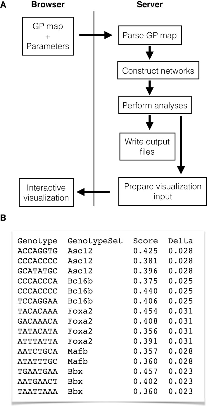
Workflow and input file. (A) Workflow, shown in terms of interaction between the browser and the Genonets Server. (B) Sample input file for empirical transcription factor binding affinity data (34). Genotypes are DNA sequences (‘Genotype’), phenotypes are the transcription factors that bind these sequences (‘GenotypeSet’), quantitative phenotypes are in vitro measures of binding affinity (‘Score’) and the noise associated with each quantitative phenotype is based on the correlation between two biological replicates of the assay (‘Delta’). ‘Genotype’ and ‘GenotypeSet’ provide the Genonets Server with necessary and sufficient information for topological analyses, whereas ‘Score’ and ‘Delta’ are additionally required for topographical analyses. If ‘Score’ and ‘Delta’ are not specified, a column of zeros must be written under these headers in the input file.

The input form

The input form allows the user to upload their genotype–phenotype map and set a small number of parameters. The format for the genotype–phenotype map is simple, and includes just the following four columns: (i) genotype, (ii) categorical phenotype, (iii) quantitative phenotype and (iv) noise associated with the quantitative phenotype. Each row in the file corresponds to a single genotype. An example is shown in Figure 2B.

The parameters to be set on the input form include: (i) the genotype alphabet. DNA, RNA, amino acid and binary sequences (e.g. wild-type versus mutant allele (28)) are supported; (ii) a lower bound τ on the quantitative phenotype, which is used to filter genotypes from genotype sets. For example, when studying RNA sequence to secondary structure maps, one may wish to ignore those sequences that have high folding energies. Alternatively, when studying transcription factor binding affinity maps (18), one may wish to ignore those DNA sequences that bind a transcription factor with very low affinity; e.g. τ = 0.35 was used in (18). 3) Allowed mutation types, where point mutations and small indels are supported. The indels we consider shift an entire contiguous sequence by a single letter (see the Supplementary Data for details). (iv) The final parameter to set is the selection of topological and topographical analyses to be performed.

Construction of genotype and phenotype networks

Genotype networks are constructed as follows. For each genotype set, the number of mutations that separate each pair of genotypes is computed. Genotypes are then represented as vertices, and pairs of vertices are connected by an edge if their corresponding genotypes are separated by a single mutation (Figure 1C).

We use the dominant genotype network of each phenotype to construct a phenotype network. In this network, dominant genotype networks are represented as vertices and pairs of vertices are connected by an edge if at least one non-neutral mutation changes a genotype from one dominant genotype network into a genotype from the other dominant genotype network (Figure 1E).

Topological analyses

Topological analyses rely upon just two columns of the input file: ‘Genotype’ and ‘GenotypeSet.’ The analyses included in the Genonets Server are based on (17,22,29).

Robustness

This quantifies the invariance of a phenotype in the face of genetic perturbation (17). Robustness is measured for individual genotypes and for phenotypes. The robustness of an individual genotype is simply the proportion of all possible single mutations that are neutral. The robustness of a phenotype is the average robustness of all genotypes in the corresponding dominant genotype network.

Evolvability

This quantifies the ability of mutations to generate novel phenotypes (17). Like robustness, evolvability is measured for individual genotypes and for phenotypes. The evolvability of an individual genotype is the proportion of all phenotypes that can be realized by single non-neutral mutations to the genotype. The evolvability of a phenotype is the proportion of all phenotypes that can be realized by single non-neutral mutations to any genotype in the corresponding dominant genotype network.

Accessibility

This quantifies the proportion of non-neutral mutations that yield a given phenotype i from phenotype j, summed across all phenotypes j ≠ i in the genotype–phenotype map (22). This measure reflects how easy it is to ‘find’ a phenotype via non-neutral mutations to genotypes that have other phenotypes.

Neighbor abundance

This quantifies the average number of genotypes in the dominant genotype networks that are adjacent to a phenotype i, scaled by the probability that non-neutral mutations yield these phenotypes (22). Neighbor abundance is high when a phenotype is mutationally biased toward phenotypes with large dominant genotype networks, and low otherwise.

Diversity index

This quantifies the probability that two randomly chosen non-neutral mutations to genotypes in the same dominant genotype network will yield genotypes with different phenotypes (22). This measure captures the diversity of phenotypes that can be accessed via non-neutral mutations from a given phenotype.

Overlap

This quantifies the number of genotypes common to a pair of dominant genotype networks. This is measured for all pairs of phenotypes in the genotype–phenotype map.

Structure

This quantifies several canonical topological properties of the dominant genotype networks, including diameter, clustering coefficient, assortativity and edge density (please see online documentation for further details).

Topographical analyses

Topographical analyses rely upon all four columns of the input file. They facilitate the exploration of a dominant genotype network as an adaptive landscape (30). Since the quantitative phenotype may be a direct measurement of organismal fitness (31), or an indirect measurement such as the minimum inhibitory concentration of an antibiotic (28), it can be used to define the ‘elevation’ of each genotype in the landscape; the noise associated with each genotype is used to determine whether two quantitative phenotypes truly differ from one another. The analyses included in the Genonets Server are based on (23–25).

Peaks

This quantifies both the number of peaks in the landscape and the number of genotypes per peak (23). This is a simple measure of landscape ruggedness.

Paths

This quantifies the number of accessible mutational paths from each genotype in a dominant genotype network to the genotype with the highest quantitative phenotype (i.e. the summit) (24). A mutational path is accessible if the quantitative phenotype increases monotonically along the path.

Epistasis

This quantifies non-additive interactions between pairs of mutations in their contribution to the quantitative phenotype. Three classes of epistasis are reported: magnitude, simple sign, and reciprocal sign epistasis, which vary in their contributions to the ruggedness of an adaptive landscape (25).

Visualization

The Genonets Server provides multiple interactive visualizations spread across different views, covering the entire spectrum of topological and topographical analyses described in the previous sections. The main view consists of the phenotype network. Clicking on one of its vertices triggers a visualization of the corresponding dominant genotype network (Figure 3, left panel), which can also be viewed as an adaptive landscape (Figure 3, right panel).

Figure 3.

Interactive visualization of a genotype-phenotype map. Data correspond to in vitro measurements of transcription factor binding affinity (34), in which genotypes are DNA sequences and phenotypes are the transcription factors that bind these sequences; a subset of these data is shown in Figure 2B. (Left panel) Topology: the phenotype network of 104 mouse transcription factors is shown on the left, in which the high mobility group protein Sox21 has been selected. The dominant genotype network for Sox21 is shown on the right, with its diameter highlighted. (Right panel) Topography: the dominant genotype network for Sox21 is shown in the landscape view. The center vertex is the summit, and each concentric ring contains genotypes of the same mutational distance from the summit, with distances increasing as the rings are read from the center outward. Vertex color represents the quantitative phenotype and vertex size represents the number of accessible mutational paths that travel through the vertex.

The phenotype and genotype network views are complemented with interactive tabular data views, where each row corresponds to a single vertex, and each column corresponds to one attribute associated with the vertices. It is possible to search for vertices based on any of these attributes. The tabular view also provides on-click creation of histograms and bar charts for plotting attributes, and scatter plots for viewing correlations between attributes. All plots are interactive. Interactivity is further supported in the form of vertex hover, selection and drag; right-clicking on a vertex enables a context menu with various analysis and visualization options. For example, right-clicking on a vertex in the phenotype network permits one to visually compare its dominant genotype network to that of another phenotype.

Output files

All attributes calculated for the topological and topographical analyses are available in easy-to-parse text files in the Tab Separated Value (TSV) format. One file provides the attributes for all phenotypes in the genotype–phenotype map, in which each row corresponds to a phenotype and each column to an attribute. Another file contains an N × N matrix that describes the overlap observed among all pairs of phenotypes. An additional file is generated for each phenotype, in which each row corresponds to a genotype with that phenotype and each column to an attribute. Moreover, the phenotype network and all dominant genotype networks are provided in the Graph Modeling Language (GML) format. This makes it possible to load the networks into external graph modeling tools, such as Gephi (32). A compressed archive of all the above-mentioned files is available for download from the visualization page.

Implementation

The server side is implemented in the Python programming language. The python-igraph package (33) is used for generic graph data structures and algorithms. The interactive visualizations are implemented in Javascript, and run entirely in the browser. This also means that the performance of the visualization is limited by the amount of processing power and available memory on the user's machine, rather than on the server.

In order to facilitate users for whom the compute capacity of the server is not enough, the code for construction and analysis of genotype networks is available as a Python package called genonets. The genonets package can be used either as a command line tool, or as an API. Please see the Supplementary Data for more details.

RESULTS

In addition to rigorous basic testing with computer-generated data, we have also tested and validated the Genonets Server on empirical genotype–phenotype maps for DNA, RNA and amino acid sequences. For binary sequences, testing and validation was performed on a genotype–phenotype map derived from a computational model. These datasets are included in the Supplementary Data. In all cases, the Genonets Server produced identical results to those previously reported.

DNA

A total of 48 290 DNA sequences (each 8 nt long) that bind 104 different transcription factors (34) were processed. The results were validated by comparing the robustness and evolvability measures against those reported in (18) and the topography measures against those reported in (Aguilar-Rodríguez, J., Payne, J. L. and Wagner, A., submitted).

RNA

A total of 15 174 RNA sequences (each 7 nt long) that bind 116 different RNA binding proteins (35) were processed. The results were validated via comparison to those from a separate codebase in our lab.

Protein

A total of 742 protein sequences (each 329 amino acids long), representing mutations in the viral hemagglutinin protein (36) were processed. The results were validated by comparing to those reported in (37).

Binary

A total of 31 870 binary sequences representing 114 different expression patterns in model gene regulatory circuits were processed. The results were validated by comparing to those presented in (38).

DISCUSSION

We have presented the Genonets Server, a tool for the construction, analysis and visualization of genotype networks. The release of our tool coincides with a dramatic increase in the availability of empirical genotype–phenotype maps (12,39–40) and with the development of ever-more sophisticated computational models used to generate genotype–phenotype maps (41). It is our hope that the Genonets Server will lower the barrier of entry to studying genotype networks in such maps, and thus aid the scientific community in basic research.

We also hope that the visualization capabilities of the Genonets Server will facilitate exploratory research. For example, one aim of synthetic biology is to develop transcriptional regulatory circuits that reliably yield a particular gene expression pattern. To achieve this goal, it is important that each transcription factor in a circuit binds only its target sites and not the target sites of other factors. The overlap feature of our tool may be used to minimize such ‘cross-talk’ (43), by determining which transcription factor binding sites are orthogonal to one another within a genotype–phenotype map of binding affinity (e.g. (18)).

Finally, we believe that the Genonets Server will be a useful pedagogical tool. It allows students to study genotype–phenotype maps and genotype networks with no development effort. Fundamental concepts, such as adaptive landscape ruggedness (42) and the relationship between robustness and evolvability (16) can be discovered with just a few mouse-clicks. What is more, our easy-to-use input form facilitates these discoveries in datasets derived from the most cutting-edge high-throughput technologies available today.

AVAILABILITY

The Genonets Server is available at http://ieu-genonets.uzh.ch. This website is free and open to all users and there is no login requirement.

SUPPLEMENTARY DATA

Supplementary Data are available at NAR Online.

FUNDING

Ambizione program of the Swiss National Science Foundation [PZ00P3-154773 to F.K., J.L.P.]; Forschungskredit program of the University of Zurich [FK-14-076 to J.A.]; Swiss National Science Foundation [31003A_146137 to A.W.]; University Priority Research Program in Evolutionary Biology at the University of Zurich. Funding for open access charge: Swiss National Science Foundation [PZ00P3-154773].

Conflict of interest statement. None declared.

REFERENCES

- 1.Alberch P. From genes to phenotype: dynamical systems and evolvability. Genetica. 1991;84:5–11. doi: 10.1007/BF00123979. [DOI] [PubMed] [Google Scholar]
- 2.van Nimwegen E., Crutchfield J.P., Huynen M. Neutral evolution of mutational robustness. Proc. Natl. Acad. Sci. U.S.A. 1999;96:9716–9720. doi: 10.1073/pnas.96.17.9716. [DOI] [PMC free article] [PubMed] [Google Scholar]
- 3.Hayden E.J., Ferrada E., Wagner A. Cryptic genetic variation promotes rapid evolutionary adaptation in an RNA enzyme. Nature. 2011;474:92–95. doi: 10.1038/nature10083. [DOI] [PubMed] [Google Scholar]
- 4.Draghi J.A., Parsons T.L., Wagner G.P., Plotkin J.B. Mutational robustness can facilitate adaptation. Nature. 2010;463:353–355. doi: 10.1038/nature08694. [DOI] [PMC free article] [PubMed] [Google Scholar]
- 5.Schuster P., Fontana W., Stadler P.F., Hofacker I.L. From sequences to shapes and back: a case study in RNA secondary structures. Proc. R. Soc. B. 1994;255:279–284. doi: 10.1098/rspb.1994.0040. [DOI] [PubMed] [Google Scholar]
- 6.Cotterell J., Sharpe J. An atlas of gene regulatory networks reveals multiple three-gene mechanisms for interpreting morphogen gradients. Mol. Syst. Biol. 2010;6:425. doi: 10.1038/msb.2010.74. [DOI] [PMC free article] [PubMed] [Google Scholar]
- 7.Salazar-Ciudad I., Marín-Riera M. Adaptive dynamics under development-based genotype-phenotype maps. Nature. 2013;497:361–364. doi: 10.1038/nature12142. [DOI] [PubMed] [Google Scholar]
- 8.Carter H., Hofree M., Ideker T. Genotype to phenotype via network analysis. Curr. Opin. Genet. Dev. 2013;23:611–621. doi: 10.1016/j.gde.2013.10.003. [DOI] [PMC free article] [PubMed] [Google Scholar]
- 9.Maynard Smith J. Natural selection and the concept of a protein space. Nature. 1970;225:563–564. doi: 10.1038/225563a0. [DOI] [PubMed] [Google Scholar]
- 10.Lipman D.J., Wilbur J.W. Modelling neutral and selective evolution of protein folding. Proc. R. Soc. B. 1991;245:7–11. doi: 10.1098/rspb.1991.0081. [DOI] [PubMed] [Google Scholar]
- 11.Hinkley T., Martins J., Chappey C., Haddad M., Stawiski E., et al. A systems analysis of mutational effects in HIV-1 protease and reverse transcriptase. Nat. Genet. 2011;43:487–489. doi: 10.1038/ng.795. [DOI] [PubMed] [Google Scholar]
- 12.Palmer A.C., Toprak E., Baym M., Kim S., Veres A., et al. Delayed commitment to evolutionary fate in antibiotic resistance fitness landscapes. Nat. Commun. 2015;6:7385. doi: 10.1038/ncomms8385. [DOI] [PMC free article] [PubMed] [Google Scholar]
- 13.Koelle K., Cobey S., Grenfell B., Pascual M. Epochal evolution shapes the phylodynamics of interpandemic influenza A (H3N2) in humans. Science. 2006;314:1898–1903. doi: 10.1126/science.1132745. [DOI] [PubMed] [Google Scholar]
- 14.Schultes E.A., Bartel D.P. One sequence, two ribozymes: implications for the emergence of new ribozyme folds. Science. 2000;289:448–452. doi: 10.1126/science.289.5478.448. [DOI] [PubMed] [Google Scholar]
- 15.Podgornaia A.I., Laub M.T. Pervasive degeneracy and epistasis in a protein-protein interface. Science. 2015;347:673–677. doi: 10.1126/science.1257360. [DOI] [PubMed] [Google Scholar]
- 16.Wagner A. Neutralism and selectionism: a network-based reconciliation. Nat. Rev. Genet. 2008;9:965–974. doi: 10.1038/nrg2473. [DOI] [PubMed] [Google Scholar]
- 17.Wagner A. Robustness and evolvability: a paradox resolved. Proc. R. Soc. B. 2008;275:91–100. doi: 10.1098/rspb.2007.1137. [DOI] [PMC free article] [PubMed] [Google Scholar]
- 18.Payne J.L., Wagner A. The robustness and evolvability of transcription factor binding sites. Science. 2014;466:714–719. doi: 10.1126/science.1249046. [DOI] [PubMed] [Google Scholar]
- 19.Banzhaf W., Leier A. Evolution on neutral networks in genetic programming. In: Yu T, Riolo R, Worzel B, editors. Genetic Programming Theory and Practice III. Boston: Springer; 2008. pp. 207–221. [Google Scholar]
- 20.Raman K., Wagner A. The evolvability of programmable hardware. J. R. Soc. Interface. 2011;8:269–281. doi: 10.1098/rsif.2010.0212. [DOI] [PMC free article] [PubMed] [Google Scholar]
- 21.Dall'Olio G.M., Vahdati A.R., Bertranpetit J., Wagner A., Laayouni H. VCF2Networks: applying genotype networks to single-nucleotide variants data. Bioinformatics. 2015;31:438–439. doi: 10.1093/bioinformatics/btu650. [DOI] [PubMed] [Google Scholar]
- 22.Cowperthwaite M.C., Economo E.P., Harcombe W.R., Miller E.L., Meyers L.A. The ascent of the abundant: How mutational networks constrain evolution. PLoS Comput. Biol. 2008;4:e1000110. doi: 10.1371/journal.pcbi.1000110. [DOI] [PMC free article] [PubMed] [Google Scholar]
- 23.Dawid A., Kiviet D.J., Kogenaru M., de Vos M., Tans S.J. Multiple peaks and reciprocal sign epistasis in an empirically determined genotype-phenotype landscape. Chaos. 2010;20:026105. doi: 10.1063/1.3453602. [DOI] [PubMed] [Google Scholar]
- 24.Franke J., Klözer A., de Visser A.J., Krug J. Evolutionary accessibility of mutational pathways. PLoS Comput. Biol. 2011;7:e1002134. doi: 10.1371/journal.pcbi.1002134. [DOI] [PMC free article] [PubMed] [Google Scholar]
- 25.Poelwijk F.J., Tanase-Nicola S., Kiviet D.J., Tans S.J. Reciprocal sign epistasis is a necessary condition for multi-peaked fitness landscapes. J. Theor. Biol. 2011;272:141–144. doi: 10.1016/j.jtbi.2010.12.015. [DOI] [PubMed] [Google Scholar]
- 26.Wagner A. Mutational robustness accelerates the origin of novel RNA phenotypes through phenotypic plasticity. Biophys. J. 2014;106:955–965. doi: 10.1016/j.bpj.2014.01.003. [DOI] [PMC free article] [PubMed] [Google Scholar]
- 27.Ciliberti S., Martin O.C., Wagner A. Innovation and robustness in complex regulatory gene networks. Proc. Natl. Acad. Sci. U.S.A. 2007;104:13591–13596. doi: 10.1073/pnas.0705396104. [DOI] [PMC free article] [PubMed] [Google Scholar]
- 28.Weinreich D.M., Delaney N.F., DePristo M.A., Hartl D.L. Darwinian evolution can follow only very few mutational paths to fitter proteins. Science. 2006;312:111–114. doi: 10.1126/science.1123539. [DOI] [PubMed] [Google Scholar]
- 29.Newman M. Networks: An Introduction. Oxford: Oxford University Press; 2010. [Google Scholar]
- 30.Wright S. Proc. 26th Int. Congr. Genet. 1932. The roles of mutation, inbreeding, crossbreeding and selection in evolution; pp. 356–366. [Google Scholar]
- 31.Lunzer M., Miller S.P., Felsheim R., Dean A.M. The biochemical architecture of an ancient adaptive landscape. Science. 2005;310:499–501. doi: 10.1126/science.1115649. [DOI] [PubMed] [Google Scholar]
- 32.Bastian M., Heymann S., Jacomy M. Proc. 3rd. ICWSM. AAAI; 2009. Gephi: An Open Source Software for Exploring and Manipulating Networks; pp. 361–362. [Google Scholar]
- 33.Csardi G., Nepusz T. The igraph software package for complex network research. InterJournal Complex Systems. 2006:1695. [Google Scholar]
- 34.Badis G., Berger M.F., Philippakis A.A., Talukder S., Gehrke A.R., Jaeger S.A., Chan E.T. Diversity and complexity in DNA recognition by transcription factors. Science. 2009;324:1720–1723. doi: 10.1126/science.1162327. [DOI] [PMC free article] [PubMed] [Google Scholar]
- 35.Ray D., Kazan H., Cook K.B., Weirauch M.T., Najafabadi H.S., et al. A compendium of RNA-binding motifs for decoding gene regulation. Nature. 2013;499:172–177. doi: 10.1038/nature12311. [DOI] [PMC free article] [PubMed] [Google Scholar]
- 36.Russell C.A., Jones T.C., Barr I.G., Cox N.J., Garten R.J., et al. The global circulation of seasonal influenza A (H3N2) viruses. Science. 2008;320:340–346. doi: 10.1126/science.1154137. [DOI] [PubMed] [Google Scholar]
- 37.Wagner A. A genotype network reveals homoplastic cycles of convergent evolution in influenza A (H3N2) haemagglutinin. Proc. R. Soc. B. 2014;281:20132763. doi: 10.1098/rspb.2013.2763. [DOI] [PMC free article] [PubMed] [Google Scholar]
- 38.Payne J.L., Wagner A. Constraint and contingency in multifunctional gene regulatory circuits. PLoS Comput. Biol. 2013;9:e1003071. doi: 10.1371/journal.pcbi.1003071. [DOI] [PMC free article] [PubMed] [Google Scholar]
- 39.Jiménez J.I., Xulvi-Brunet R., Campbell G.W., Turk-MacLeod R., Chen I.A. Comprehensive experimental fitness landscape and evolutionary network for small RNA. Proc. Natl. Acad. Sci. U.S.A. 2013;110:14984–14989. doi: 10.1073/pnas.1307604110. [DOI] [PMC free article] [PubMed] [Google Scholar]
- 40.Weirauch M.T., Yang A., Albu M., Cote A.G., Montenegro-Montero A., et al. Determination and inference of eukaryotic transcription factor sequence specificity. Cell. 2014;158:1431–1443. doi: 10.1016/j.cell.2014.08.009. [DOI] [PMC free article] [PubMed] [Google Scholar]
- 41.Greenbury S.F., Johnson I.G., Louis A.A., Ahnert S.E. A tractable genotype-phenotype map modelling the self-assembly of protein quaternary structure. J. R. Soc. Interface. 2014;11:20140249. doi: 10.1098/rsif.2014.0249. [DOI] [PMC free article] [PubMed] [Google Scholar]
- 42.Kauffman S., Levin S. Toward a general theory of adaptive walks on rugged landscapes. J. Theor. Biol. 1987;128:11–45. doi: 10.1016/s0022-5193(87)80029-2. [DOI] [PubMed] [Google Scholar]
- 43.Friedlander T., Roshan P., Guet C.G., Barton N.H., Tkačik G. Intrinsic limits to gene regulation by global crosstalk. arXiv. 2015 doi: 10.1038/ncomms12307. 1506.06925. [DOI] [PMC free article] [PubMed] [Google Scholar]
Associated Data
This section collects any data citations, data availability statements, or supplementary materials included in this article.