Abstract
We compare the speed and effectiveness of two genetic optimization algorithms to the results of statistical sampling via a Markov chain Monte Carlo algorithm to find which is the most robust method for determining real space structure in periodic gratings measured using critical dimension small angle X-ray scattering. Both a covariance matrix adaptation evolutionary strategy and differential evolution algorithm are implemented and compared using various objective functions. The algorithms and objective functions are used to minimize differences between diffraction simulations and measured diffraction data. These simulations are parameterized with an electron density model known to roughly correspond to the real space structure of our nanogratings. The study shows that for X-ray scattering data, the covariance matrix adaptation coupled with a mean-absolute error log objective function is the most efficient combination of algorithm and goodness of fit criterion for finding structures with little foreknowledge about the underlying fine scale structure features of the nanograting.
Keywords: X-ray scattering, nanostructure metrology, genetic algorithm, covariance matrix adaptation evolutionary strategy, differential evolution, Markov chain Monte Carlo
1 Introduction
The recent progression of information processing technology moving toward device components with smaller and smaller feature sizes has required the advent of novel metrology methods for characterizing the fine details of those nanostructures. Traditional photolithographic fabrication methods have started to reach fundamental limits in the size of features they can produce1–3 and the next generation methods such as extreme ultraviolet lithography4,5 have many lingering issues needing to be addressed to become economically viable6,7. Thus, alternative lithographic methods such as block copolymer (BCP) directed self-assembly (DSA)8–13, direct write focused ion or electron beam14,15, or other multistep patterning photolithography techniques16–18 are necessary to continue the trend predicted by Gordon Moore of device density doubling every couple of years19. In particular, BCP DSA can be quite prone to defects20 and poor long-range order21,22 compared to traditional lithography, and as a result better metrology techniques for measuring the overall order need to be implemented. Regardless of the fabrication method chosen, precisely characterizing the structures made at these sub-10 nm dimensions is critical for ensuring quality control and device performance.
Current methods for characterizing defects in thin film BCPs include a combination of optical defect detection with scanning electron microscopy (SEM)23, scatterometry or optical critical dimension (OCD) metrology24, and X-ray scattering metrology using critical dimension small angle X-ray scattering (CDSAXS)25–30 with resonant soft X-rays31–35. SEM is most useful for detecting defects related to pattern registration, where deviations from the patterned template are visible at the surface. However, simulation studies have shown that for BCP thin films, deviations in the through-film morphology can be present below the top surface36 and thus not be discernable by scanning electron microscopy. CDSAXS on the other hand has demonstrated the capability for detecting periodic buried structure morphologies that differ from a desired uniform grating34 but requires an inverse algorithm to convert the scattering intensity data into a meaningful real space structure. If the goal is having fast turn-around non-destructive characterization of detailed internal structures (with many model parameters), then traditional optimization refinement methods are not practical due to the long run times necessary to solve and test simulated scattering data iteratively and the very real possibility of identical-cost, degenerate structural solutions (common to scattering analysis). Thus an optimization algorithm that converges to the global best fit quickly and consistently is desired. Supplemental knowledge of the underlying structure can expedite this process and has to be used to some degree in model design, but such sample knowledge is not always readily available.
Previous studies33–35 have used a Markov chain Monte Carlo (MCMC) algorithm37 to determine the parameter set for the given structure model that best fits the measured scattering data. This approach requires a relatively good initial guess with tight parameter search bounds for the structure parameters and requires multiple independent chain runs to ensure the algorithm has convergence. However, the potential for fabrication errors require larger parameter search bounds to ensure the solution found is the actual structure; thus such an approach may not be able to distinguish a potential faulty sample. Approaches have also been tried that use massive computing resources with parallelization and highly refined grid based models with a reverse MCMC38, but such an approach is limited by the availability of the computing resources. Genetic and evolutionary based algorithms have shown the capability to search large parameter spaces with wide bounds successfully. These algorithms mimic biological evolution using the model parameter sets as the encoding genetic information that is then processed through some kind of mixing strategy over many generations until the optimal parameter set evolves from an initial set of randomly generated parameters39. The mixing strategy can be simple such as in a differential evolution (DE)40 approach or more complicated such as in the covariance matrix adaptation evolutionary strategy (CMAES)41–43. These methods are better suited to search a wider parameter space than stochastic algorithms like the MCMC. Previous work44,45 used an MCMC-like approach to determine the positions of post motifs directing the self-assembly of BCPs into complex patterns and required many runs that were averaged over space to find the most optimal solutions that yielded the desired target structure morphology. Similar work was performed using chemical spot motifs using a CMAES algorithm that showed convergence to global solutions was possible consistently within a reasonable number of algorithm generations46,47.
In this work, we compare these methods of inverse structure determination from CDSAXS measurements using MCMC, DE, and CMAES algorithms. First, the algorithms are compared by fitting the parameters of model target structures with simulated intensity profiles, starting from random initial parameters and typical parameter search ranges. Next, a set of experimental data from a silicon nanograting made using a BCP mask pattern transfer was used to compare the three algorithms, which were also compared with the results previously found using this data and only an MCMC approach. Additionally, a series of objective functions are investigated for each algorithm to see how the high dynamic range of scattering intensity measurements affects convergence of model parameters. Similar high dynamic range data is encountered in other problems where inverse solutions are needed such as X-ray or neutron reflectivity48, ellipsometry49,50, scatterometry/OCD metrology51, or seismic surveying52,53, thus the methods presented should be applicable in those fields as well. The results of these various runs are compared to infer which algorithm and objective function combination is best suited for optimized fitting of scattering data in terms of both refinement speed and convergence robustness.
2 Methods
2.1 Inverse Algorithms
The three different methods tested were the MCMC, DE, and CMAES algorithms. Here we detail general parameters and procedures that are shared between the three methods. Details of each algorithm, how the internal parameters for each algorithm were chosen and optimized, and any nuances each algorithm presents to the problem of inverse structure determination are provided in the appendices (see Appendix A).
For all the inverse algorithms considered, the goal is to find a set of model parameters that best parameterizes the real space structure of the sample investigated via CDSAXS intensity measurements. The model parameter set contains NShape parameters describing the geometric positions of the defining features in the periodic structure of the thin film and the relative magnitude of the scattering length density, SLD ≡ ρ(r⃗), of the material as a function of those geometric positions. Additionally, three intensity scaling parameters are included to properly scale the simulated intensities with the measured experimental intensities and account for interfacial roughness, giving the total model parameters needed for a given structure as NParam = NShape + 3. Model parameter indices are denoted as κ = 1, …, NParam. These model parameters are stored in a vector P⃗G,C, where the index G represents the current iteration in the case of MCMC or generation for the genetic algorithms and C is either the chain number in the MCMC algorithm or individual index of the population in the genetic algorithms.
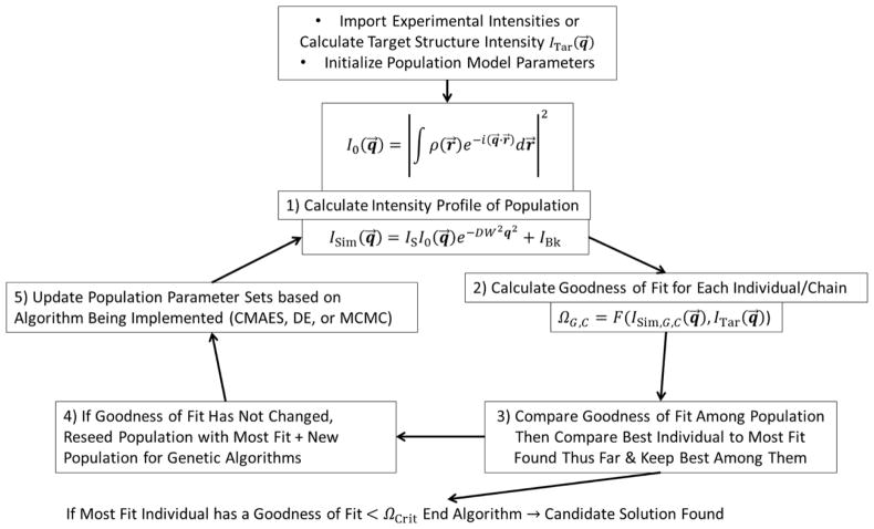
A general outline of the methodology is shown in Fig. 1. The approach is initiated by choosing which inverse optimization algorithm to use, selecting what kind of geometric model to use (and thus how many NParam are needed), initiating model parameters within the relevant bounds, picking the kind of objective function to be used to measure goodness of fit Ω, importing the experimental (or simulated) target intensity profile, and simulating an intensity profile for a test model parameters set. The main algorithm then commences as follows: 1) The scattering intensity profile for each model parameter set P⃗G,C within the population (for the genetic algorithms) or for the current step of the chain set (for the MCMC) is simulated yielding ISim,G,C(q⃗), the simulated scattering intensity as a function of the reciprocal space vector q⃗ = [qx, qz] for Nq qx and qz values. 2) The goodness of fit Ω is calculated for ISim,G,C(q⃗) with the experimental or target intensity profile ITar(q⃗). 3) Depending on the exact algorithm used, a comparison is made between Ω values of previous iterations/generations, amongst P⃗G,C in the current population, or a best found “most fit” P⃗MF and a decision is made on how to proceed with the algorithm. 4) For the genetic algorithms, if the population has bottlenecked into a constant Ω solution not less than ΩCrit (based on the average change in the goodness of fit over a fixed number of generations (chosen here as 20) staying below a predefined small value (chosen here as 10−2)), the population is reseeded keeping the best model parameter set P⃗MF but reinitializing all other model parameter sets. This step generally occurs after the solution parameter set is already very close to the best solution, thus the aggressiveness of the step is only for fine refinement of the solutions. 5) The algorithm being used is implemented to modify P⃗G,C based on the decision of the Ω comparison. These steps are repeated each time using the modified P⃗G,C in the first step until either a convergence criterion is reached (i.e. a predetermined value for Ω = ΩCrit that is deemed an acceptable solution; ΩCrit is usually determined by running a few preliminary algorithm runs and seeing what the Ω values starts to converge towards such that only a few accepting events occurs within several hundred generations, otherwise ΩCrit is just set to 0) or for a preset number of generations/iterations.
Fig. 1.
Diagram outlining the major steps in our approach. This format is general for different objective functions and different parameter set updating algorithms (CMAES, DE, or MCMC).
2.2 Modeling Scattering Length Density
In order to simulate scattered intensity profiles, an appropriate model must be used to convert ρ(r⃗) into a shape profile that can be defined in a set of parameters of size NParam. In general, the simulated intensity is written as
| (1) |
where IS is an intensity scaling parameter, DW is the Debye-Waller factor, IBk is the background intensity, and I0(q⃗) is the amplitude squared of the Fourier transform of ρ(r⃗) such that
| (2) |
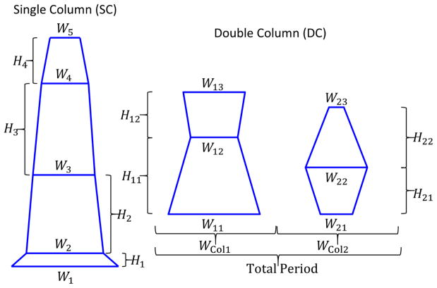
For this study, a model using stacks of trapezoids was used. In the model, a system of M trapezoids is used to represent ρ(r⃗) each with their own SLD = ρm, bottom width WB,m, top width WT,m, height Hm, and position of the bottom left corner in x and z (xm, zm). Here m is an index for the mth trapezoid. In principle each trapezoid is defined by 6 parameters, but generally constraints are assumed with trapezoids in the same stack having the same parameters defined for adjoining sides and one trapezoid has a corner defined as the origin, thus the actual total number of parameters will be less than 6M. Additional details of how the intensities for the trapezoid model simulated intensities are calculated are in the appendices (see Appendix B). Fig. 2 shows how example composite shape profiles are developed from the trapezoid model with both single column (SC) and double columns (DC) of trapezoidal stacks. Details of how these model parameters are related and determined are also discussed in the appendices (see Appendix B).
Fig. 2.
Example trapezoid model based shape profiles used in calculating the SLD for the target intensities. The two main types of model parameter sets explored are those of a single column of periodic trapezoid features shown on the left (SC) and those of double columns of periodic features shown on the right (DC). Geometric model parameters are denoted in the figure.
2.3 Objective Function – Goodness of Fit
In order to find an optimal set of parameters producing a simulated intensity profile which most closely matches the experimental or target structure intensity profile, an objective function that properly captures the goodness of fit needs to be selected. The symbol Ω is defined as the measure of the goodness of fit for a general objective function. Each specific objective function then has its own designated symbol. Depending on the data being sampled and compared, various objective functions may be appropriate. For the intensity data examined in CDSAXS experiments, the sampled data can cover orders of magnitude in values suggesting some logarithmic objective function may be appropriate. At the same time, Poisson noise is expected to dominate the measured intensity values in terms of random error, suggesting a χ2 objective function might be appropriate. Based on these facts, we chose to use three functions in the algorithm comparison study: χ2, a mean-absolute error logarithmic function, and a mean-absolute error function as a control. It should be noted that a parameter set that gives a minimum using one objective function does not necessarily give a minimum for other objective functions; thus the proper selection of an objective function that precisely embodies the goodness of fit for all the data is essential to inverse structure determination.
2.3.1 χ2 goodness of fit
The χ2 goodness of fit objective function is a standard objective function that compares the square difference of values in the measured data and the simulated data normalized to the expected model value (treated here as the simulated value). In our intensity simulation studies, the following form of χ2 was used:
| (3) |
χ2 works best for cases where the error in the data obeys a Poisson distribution.
2.3.2 Mean-absolute error log goodness of fit
The mean-absolute error log (MAElog) goodness of fit objective function is a standard objective function that compares the difference of the logarithm of the values in the measured data and the simulated data54. In our intensity simulation studies, the following form of this objective function was used:
| (4) |
This objective function is best suited for data that has values that span many orders of magnitude which is true for scattering intensity data where the primary peak can be many orders of magnitude larger than the higher order peaks40. When compared with a mean-squared error type function, this function has been shown to be less sensitive to statistical noise40.
2.3.3 Mean-absolute error goodness of fit
The mean-absolute error (MAE) objective function is another common cost function which incorporates elements of both χ2 and MAElog. The MAE objective function can be appropriate for X-ray diffraction measurements when there is important information in the lower order peaks (i.e. the largest intensities)40. Mathematically this function is written as:
| (5) |
This function is essentially the sum of the absolute value of the residuals between the data and simulated fit data.
2.4 Algorithm Comparison Methodology
To test the three algorithms and their ability to converge to acceptable parameter solutions for target scattered intensities, two approaches were devised. In the first approach, various target shape profiles built from trapezoids were constructed using defined parameter sets and used to create a simulated ITar(q⃗) for testing the algorithms. Poisson noise typical to that of measured data was added to the simulated structure intensities to make the data more realistic and avoid having sharp features in the solution space (see Appendix C for how this noise was added to the simulated data). In the second approach, experimental data previously studied using an MCMC algorithm was fit with trapezoid models using all three algorithms. The success of the different algorithm and objective function combinations were measured based on two primary criteria: the magnitude of the best goodness of fit converged by that algorithms ΩBest and the normalized time to converge tConv/τGen to within a given target goodness of fit value ΩTar. tConv, the absolute time for an algorithm to converge within ΩTar, is the number of generations/iterations to converge GConv multiplied by τα, the average CPU time per generation/iteration for a given algorithm α, such that tConv = GConvτα. This value is normalized by the average time of a CMAES generation τGen (CMAES generation time was chosen arbitrarily for the normalization as any algorithm could have been used) such that τGen = τCMAES ≅ 0.95τDE ≅ 1.17τMCMC. In other words, a single step or generation in all three algorithms takes nearly an identical amount of time. ΩTar is defined for the simulated structures as 1.1 times the theoretical goodness of fit ΩConv for an exact match (found by removing the simulated Poisson noise from the simulated intensities) and 1.1 times ΩBest for the experimental data. This corresponds to a 10 % range of error in the converged goodness of fit values which will be shown to be reasonable for the parameters examined in the results and discussion section. The algorithms were run using MATLAB® (R2014b) code on a system with dual 8 core processors (Intel® Xeon® E5-2687W v2) with 3.4 GHz clock speed†.
3 Results and Discussion
Here we present the results of using all three algorithms and objective functions. We then discuss which algorithm and objective functions worked best for the different data. For the genetic algorithms, the population size was always fixed to psize =96 for consistent comparison. 96 parallel chains were used in the MCMC runs to be comparable with the genetic algorithms.
3.1 Simulated Structure Results
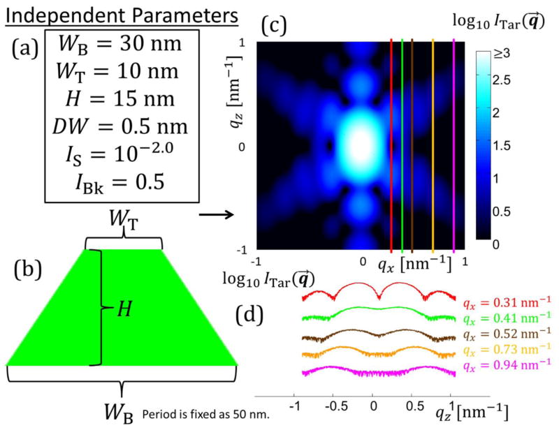
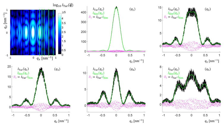
For the target simulated data case, an initial test was done using a single trapezoid with NParam = 6 and refinements were performed varying these NParam. Fig. 3 shows the parameters for this structural model and the intensity data produced for fitting by the algorithms. Bounds for fitting of the model parameters were chosen for each parameter and are detailed in the appendices (see Appendix C). To correspond to previous studies of such systems33–35, only a selection of data was used to fit the parameters, with five constant qx values being used to extract the intensity as a function of qz for those five constant values (see Fig. 3(d)). Each slice each contained 1001 data points for each ITar(qz) for a total Nq =5005 among the 5 qz slices. qz was varied from ≈ −1.0451 nm−1 to 1.0451 nm−1 in steps of 0.00209 nm−1 which is a similar resolution and range of values to those measured experimentally. Experimentally this qz range is a function of the qx resolution and angle step size as the experimental data is reconstructed from qxz slices at different X-ray incidence angles. The qx values for the slices were chosen to have a good range in intensity order of magnitude to reflect how such differences are encountered in experiments. Background noise was simulated as a constant plus Poisson distributed random noise, emulating detector read out noise behavior. Once the target data was simulated, our inverse methodology was implemented with parameters initiated randomly for the given population in the case of CMAES or DE or chain set for MCMC and the algorithm cycled until a solution close to the actual parameters was found with Ω saturating within the ΩTar value. Fig. 4 shows a representative set of fits using the CMAES algorithm with Ξ objective function for a DC structure with M = 2 (NParam = 13). The test fits, the target simulated data, and the residuals between the fit data and target simulated data are all plotted.
Fig. 3.
Schematic diagram of how known solution intensities were produced. (a) Set of independent parameters is defined for the real space structure with various geometric parameters and intensity scaling parameters. In this case three geometric parameters are required to define the bottom width WB, top width WT, and height H of a single symmetric trapezoid plus the three intensity scaling parameters DW, IS, and IBk. (b) Schematic diagram of the shape profile of the single trapezoid target structure. (c) Simulated intensity over the range of qx and qz values varying from ≈ −1 nm−1 to 1 nm−1. Intensity is plotted on a log scale for better contrast. Lighter blue regions are higher intensity and darker blue to black regions are low intensities. The five colored lines are the five intensity qz slices chosen for the inverse algorithm to use to solve for the structure. (d) Plots of the five intensity slices used in the inverse algorithm with the same coloring as from (c) with the respective qx values colored appropriately. Scaling of the intensity values is arbitrary to get all five curves onto one plot without overlapping.
Fig. 4.
Comparison of plots of the intensity fits found by the CMAES algorithm with Ξ function for the DC M = 2 target structure. Top left shows the entire simulated intensity profile with the green lines being where the qz slices were taken. The rest of the figure shows the simulated data ITar with Poisson noise plotted in black, a fit curve ISim plotted in green, and the residuals RI = ITar − ISim between the fit and simulated data with noise plotted in magenta (q1) Slice 1 qx = 0.31 nm−1. (q2) Slice 2 qx = 0.41 nm−1. (q3) Slice 3 qx = 0.52 nm−1. (q4) Slice 4 qx = 0.73 nm−1. (q5) Slice 5 qx = 0.94 nm−1.
For the case of a single trapezoid with dimensions defined in Fig. 3, NRuns = 10 runs were performed using all three algorithms each with the three objective functions for a maximum of 10000 generations each run. To quantify the performance of the different algorithm and objective function combinations, tConv/τGen and ΩBest were compared. These values are shown for the single trapezoid structure in Table 1. The tConv/τGen values here are averaged over the 10 runs with the ΩBest values being the minimum observed for all 10 runs. The values for ΩTar here were chosen such that the goodness of fit had converged within 10 % of the theoretical ΩConv value (i.e. ΩTar =1.1ΩConv) found using the intensities with noise as ITar and without noise as ISim. This convention was used for all three objective functions, so since each objective function scales goodness of fit differently, strict comparisons should only be made within the same objective function basis when considering convergence rates. The CMAES clearly outperformed in tConv/τGen, followed by the DE and then MCMC. In terms of ΩBest, both genetic algorithms reached similar best values while the MCMC tended to not refine exactly to the same value. However, the values converged towards were below or close enough to ΩConv to be deemed an acceptable solution. For the χ2 and Ξ objective functions, the actual ΩBest values found were even better than ΩConv. This just means the parameters converged toward are slightly different than the actual parameter set without noise but are still acceptable solutions.
Table 1.
Comparison of the normalized time to converge tConv/τGen within the given ΩTar value and the best ΩBest saturated goodness of fit values for the various algorithm and objective function combinations. Values of tConv/τGen are reported with standard uncertainty and averaged from all runs. ΩTar and ΩConv are listed for each objective function on the right for reference.
| CMAES | DE | MCMC | ΩTar | ΩConv | ||
|---|---|---|---|---|---|---|
| χ2 | tConv/τGen | 45 ± 4 | 230 ± 20 | 650 ± 70 | 463.5 | 421.3 |
| ΩBest | 412.1 | 412.1 | 412.9 | |||
| ψ | tConv/τGen | 50 ± 6 | 160 ± 30 | 510 ± 40 | 2307 | 2097 |
| ΩBest | 2097 | 2097 | 2098 | |||
| Ξ | tConv/τGen | 35 ± 2 | 80 ± 10 | 520 ± 40 | 514.0 | 467.2 |
| ΩBest | 465.6 | 465.6 | 465.7 | |||
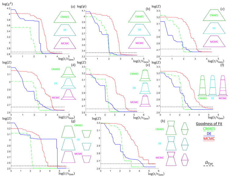
To examine how the algorithms perform with increasing NParam, additional simulations were performed with SC trapezoid stacks of size M = 2 to 4 (NParam = 8,10, and 12) as well DC stacks of one and two trapezoids with fixed column widths (NParam = 9 and 13) using the Ξ objective function. 10 runs were performed for each case for a maximum of 200000 generations. Fig. 5 shows plots of ΩBest versus t/τGen for the different numbers of parameters with the ΩTar lines added to see where the target goodness of fit values are reached for each algorithm along with the corresponding shape profile used to simulate the intensity data. The CMAES algorithm clearly outperforms the DE and MCMC by ≈ 1 to 2 orders of magnitude in speed for all NParam. The DE algorithm generally descends faster to start relative to the CMAES, but the CMAES always at some point descends in goodness of fit rapidly overtaking the DE and MCMC. This observation is due to the way the CMAES converges once the covariance matrix is well developed after several generations43. As NParam increases, the CMAES and DE continues to converge consistently toward the lowest Ω values, while the MCMC starts to take exponentially longer to get to those lowest Ω values after converging below ΩTar. Examining the target shape profiles (dotted black lines) with the solution shape profiles (colored lines), the solution shape profiles found match exactly for all targets except for the SC M = 4 with the MCMC where there is a slight mismatch in the placement of the bottom of the middle trapezoid (however, the overall shape matches well) and for the DC M = 2 with the MCMC where there are a couple of slight shifts in the trapezoid dimensions. The MCMC would likely eventually converge better for these cases with many more generations, but seeing each generation takes around 1 s to 2 s to run and 200000 generations or ≈ 4.6 d of computation time were already performed compared to the CMAES converging within an hour, continuing to run the algorithm for such further refinement was deemed unnecessary. Also, the DE takes longer to finally converge for the DC M = 1 case likely due to the search space for this structure having a local solution minimum in which the algorithm is staying. Additional discussion of the performance of the different algorithms with NParam and number of columns plus all goodness of fit trajectory plots are given in the appendices (see Appendix D).
Fig. 5.
Plots of the best (lowest goodness of fit found from up to 10 runs) run goodness of fit values versus normalized time for different number of parameter structures using the three different algorithms (CMAES in green dash dotted lines, DE in blue solid lines, and MCMC in red dotted lines). Plots are log scale. ΩTar thresholds are shown as a black dashed line. Target shape profiles (black dashed lines) and solution shape profiles (CMAES in green, DE in cyan, and MCMC in magenta) are shown to the right of each corresponding Ω versus t/τGen plot. (a–c) NParam =6 SC M = 1. (a) Ω → χ2 (b) Ω → ψ (c) Ω → Ξ (d–h) Ω → Ξ (d) NParam = 8 SC M = 2. (e) NParam = 10 SC M = 3. (f) NParam = 12 SC M = 4. (g) NParam = 9 DC M = 1. (h) NParam = 13 DC M =2.
3.2 Experimental Structure Results
For experimental comparison, a data set with intensity ITar(qz) for four qx values that was used previously for determining a structure with multiple chain runs of an MCMC algorithm35 was chosen to compare the efficiency and effectiveness of the different algorithms. The previous study found a stack of M = 3 trapezoids to yield an appropriate fit for the silicon lines formed from the pattern transfer of a block copolymer template, but for comparison with that study stacks of size M = 1 to 5 were additionally tested. The parameters that yielded the lowest goodness of fit solutions found in this study using the CMAES algorithm with Ξ objective function are shown and compared in Table 2. These results show the CMAES yielded a similar solution but with a lower Ξ value for M = 3 (normalized here by Nq − 1= 2792), slightly better fit with M = 4 trapezoids, and slightly worse fit with M = 5. Additional details of these comparisons are in the appendices (see Appendix D).
Table 2.
Comparison of various parameters found for symmetric periodic silicon grating line structure found using experimental data. CMAES with Ξ was used (normalized by Nq − 1 here). The parameters presented are the ΩBest values. For the cases of M = 1, 2, 4, and 5 only the total height HTot and full width at half max height WFWHM were compared since the individual trapezoid components making up the structure in those cases are not comparable.
| Parameter | M = 1 | M = 2 | M = 3 | M = 4 | M = 5 | Previous Study M = 3 |
|---|---|---|---|---|---|---|
| HTot [nm] | 25.66 | 26.65 | 26.55 | 26.97 | 26.73 | 26.24 |
| WFWHM [nm] | 13.55 | 13.85 | 13.87 | 13.92 | 13.97 | 14.19 |
| DW [nm] | 1.51 | 1.29 | 1.20 | 1.20 | 1.25 | 1.26 |
| IExp | −2.33 | −2.34 | −2.36 | −2.36 | −2.33 | −2.22 |
| IBk | 0.76 | 0.65 | 0.64 | 0.64 | 0.65 | 0.49 |
| ΩBest → Ξ | 0.236 | 0.199 | 0.186 | 0.185 | 0.187 | 0.195 |
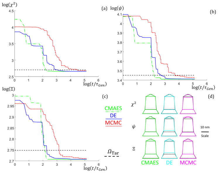
To examine the speed of the algorithms in the experimental case, plots of the goodness of fit Ω values as a function of t/τGen for the runs that yielded ΩBest upon completion are shown in Fig. 6. From the plots, the CMAES converged to a solution ≈ 1 to 2 orders of magnitude in time faster than the MCMC and less than an order of magnitude faster than the DE for the experimental structure for all objective functions. Fig. 6 also shows plots of the best shape profile fits (colored lines) for different combinations of algorithm and objective function used compared with the previously found solution (dashed black lines). The CMAES fits matched well with the previous study for all objective functions, the DE relatively well, and the MCMC only well for the Ξ objective function. These discrepancies are likely due to a combination of the χ2 and ψ weighing the first order slice too much compared to the higher ordered slices while the Ξ objective function weighs them more evenly, as shown in Table 3, and the MCMC not completely converging. Since the higher order peaks contain the information on the finer details of the periodic nanostructures (i.e. dfeature ∝ q−1), knowing how the objective function used weighs the calculated goodness of fit is important in deciding if a parameter solution set is an appropriate fit to the measured data. Thus, the fact that the Ξ function weighs the higher order peaks more appropriately in addition to giving a similar shape profile to the previously reported solution for all the algorithms gives credence to it being the best objective function for analyzing X-ray scattering data.
Fig. 6.
(a–c) Goodness of fit versus t/τGen results with M = 3 for the experimental data structure between the three algorithms (CMAES in green dash dotted lines, DE in blue solid lines, and MCMC in red dotted lines). Data is plotted on a log base 10 scale. Plots are best (lowest goodness of fit) data sets from 10 runs. (a) χ2 objective function was used. (b) ψ objective function was used. (c) Ξ objective function was used. (d) Geometric structure shape profiles for the best parameter set solutions found using the different objective functions (rows top to bottom are χ2, ψ, and Ξ) and algorithms (columns left to right are green for the CMAES, cyan for DE, and magenta for MCMC) for the M = 3 experimental data structure. Scale is inset on the right of the figure. The overlaid dotted black line structure is the solution found from the previous MCMC study for comparison.
Table 3.
The relative fractional percentage each slice contributed to the total goodness of fit for each Ω in its own basis using the CMAES algorithm. Values are calculated using the objective function noted at the top of table.
| χ2 | ψ | Ξ | |
|---|---|---|---|
| % Slice qj Contributes to Total Ω | |||
| q1 (qx =0.223 nm−1) | 99.5 % | 91.0 % | 48.3 % |
| q2 (qx =0.451 nm−1) | 0.3 % | 4.5 % | 42.2 % |
| q3 (qx =0.677 nm−1) | 0.1 % | 2.9 % | 4.5 % |
| q4 (qx =0.905 nm−1) | 0.1 % | 1.6 % | 5.0 % |
When comparing between algorithms for these simulations, there does not appear to be any correlation in a particular peak slice having a better fit with a particular algorithm; only when changing the objective function used do such discrepancies arise. Based on the fact the Ξ objective function gave the best match to the previous work, that objective function is expected to fit this kind of scattered intensity data most accurately in terms of weighing residual contributions from different peaks with large order of magnitude differences. For both the simulated structure and experimental data algorithm tests, the CMAES was determined to be the best algorithm to use for fast convergence to an accurate parameter set solution with basically no need to have an accurate starting solution population set.
4 Conclusion
The results of both the experimental and simulated structure studies demonstrate the CMAES algorithm converged most rapidly and reliably to an acceptable solution, the DE did so reliably as well, but at a slower rate, and the MCMC mostly converged to an acceptable solution but at the slowest rate. Higher structure model parameters resulted in longer computation time for all algorithms and slightly higher ΩBest values for the DE and MCMC compared to the CMAES but still gave acceptable solutions for the highest parameter numbers tested (i.e. ΩBest < ΩTar). For the experimental data tested, the CMAES with Ξ objective function gave the best match with the previously determined model parameters from an MCMC study35.
Seeing that the CMAES algorithm generally had a faster absolute time to converge to solutions and always had the lowest observed ΩBest values for the various objective functions, the algorithm shows great promise in advancing X-ray scattering metrology. With the insight gained from this study of genetic algorithms in analyzing CDSAXS data, future studies will be able to utilize these methods to analyze data quickly and efficiently with little foreknowledge of the internal structure. This current study only examined parameterized structures with up to 13 independent parameters, so future studies should examine the efficiency of the algorithms at shape models with NParam in the range of 20 to 100. There may be further algorithm enhancements than those posited here such as hybrid algorithms (e.g. using the CMAES to find the relative location of the parameter solution and honing in on better solutions with a local MCMC algorithm with tighter parameter bounds or Levenberg-Marquardt algorithm55), making structure reconstruction more tractable and deterministic. Overall, the results of this study show the CMAES algorithm will enhance X-ray scattering in turn-around time for inverse complex structure determination.
Fig. 10.
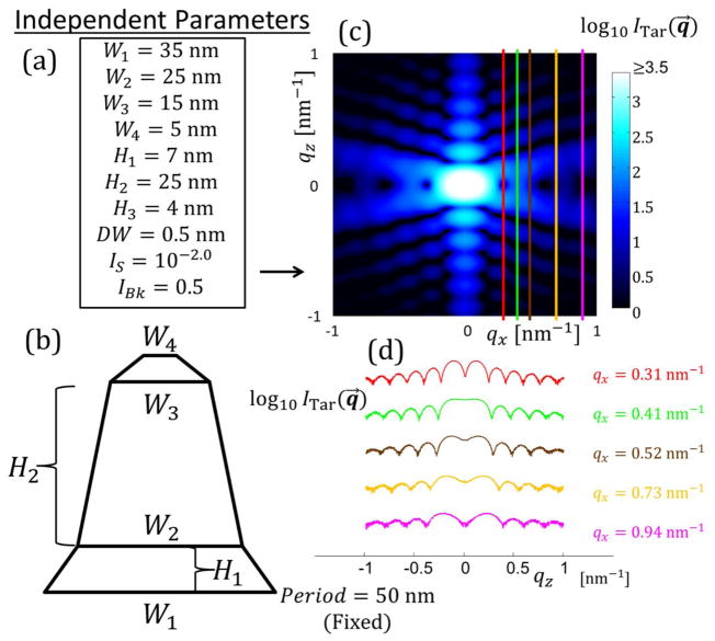
Figure analogous to Figure 3 in the main text for target structure with SC M = 3. Period is fixed as 50 nm. (a) Independent parameters defined for the SC M = 3 structure. (b) Schematic diagram of the shape profile for the SC M = 3 structure. (c) The simulated target structure intensity profile in qz versus qx for a range of [−1:1] nm−1. Intensity is plotted on a log scale with scale shown. Colored lines are constant qx cuts used for parameter optimization with the algorithms corresponding to the intensities shown in (d). (d) Log of target structure intensity slices used for fitting. Scale is arbitrary so the curves all fit on the same plot.
Fig. 11.
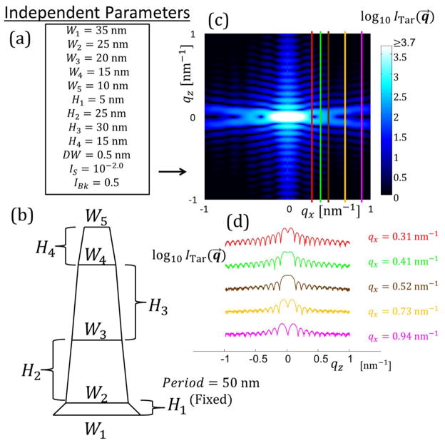
Figure analogous to Figure 3 in the main text for target structure with SC M = 4. Period is fixed as 50 nm. (a) Independent parameters defined for the SC M = 4 structure. (b) Schematic diagram of the shape profile for the SC M = 4 structure. (c) The simulated target structure intensity profile in qz versus qx for a range of [−1:1] nm−1. Intensity is plotted on a log scale with scale shown. Colored lines are constant qx cuts used for parameter optimization with the algorithms corresponding to the intensities shown in (d). (d) Log of target structure intensity slices used for fitting. Scale is arbitrary so the curves all fit on the same plot.
Fig. 12.
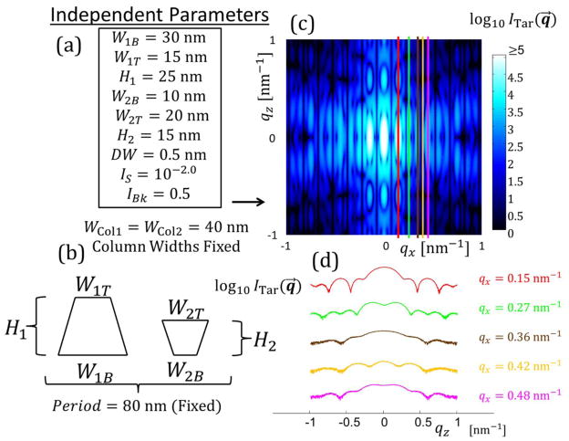
Figure analogous to Figure 3 in the main text for target structure with DC M = 1. Period is fixed as 80 nm. (a) Independent parameters defined for the DC M = 1 structure. (b) Schematic diagram of the shape profile for the DC M = 1 structure. (c) The simulated target structure intensity profile in qz versus qx for a range of [−1:1] nm−1. Intensity is plotted on a log scale with scale shown. Colored lines are constant qx cuts used for parameter optimization with the algorithms corresponding to the intensities shown in (d). (d) Log of target structure intensity slices used for fitting. Scale is arbitrary so the curves all fit on the same plot.
Table 5.
Target parameters with bounds used for SC M = 2 trapezoids target structure. Units for Wj, Hj, and DW are all in nm.
| SC M = 2 | W1 | W2 | W3 | H1 | H2 | DW | IExp | IBk |
|---|---|---|---|---|---|---|---|---|
| Parameter Value | 30 | 20 | 7 | 5 | 15 | 0.5 | −2 | 0.5 |
| Lower Bound | 1 | 1 | 1 | 1 | 1 | 0 | −5 | 0.01 |
| Upper Bound | 40 | 40 | 40 | 40 | 40 | 2 | 0 | 1 |
Table 6.
Target parameters with bounds used for SC M = 3 trapezoids target structure. Units for Wj, Hj, and DW are all in nm.
| SC M = 3 | W1 | W2 | W3 | W4 | H1 | H2 | H3 | DW | IExp | IBk |
|---|---|---|---|---|---|---|---|---|---|---|
| Parameter Value | 35 | 25 | 15 | 5 | 7 | 25 | 4 | 0.5 | −2 | 0.5 |
| Lower Bound | 1 | 1 | 1 | 1 | 1 | 1 | 1 | 0 | −5 | 0.01 |
| Upper Bound | 40 | 40 | 40 | 40 | 40 | 40 | 40 | 2 | 0 | 1 |
Table 7.
Target parameters with bounds used for SC M = 4 trapezoids target structure. Units for Wj, Hj, and DW are all in nm.
| SC M = 4 | W1 | W2 | W3 | W4 | W5 | H1 | H2 | H3 | H4 | DW | IExp | IBk |
|---|---|---|---|---|---|---|---|---|---|---|---|---|
| Parameter Value | 35 | 25 | 20 | 15 | 10 | 5 | 25 | 30 | 15 | 0.5 | −2 | 0.5 |
| Lower Bound | 1 | 1 | 1 | 1 | 1 | 1 | 1 | 1 | 1 | 0 | −5 | 0.01 |
| Upper Bound | 40 | 40 | 40 | 40 | 40 | 40 | 40 | 40 | 40 | 2 | 0 | 1 |
Table 8.
Parameters with bounds used for DC M = 1 trapezoid per column target structure. Units for Wj, Hj, and DW are all in nm.
| DC M = 1 | W1B | W1T | H1 | W2B | W2T | H2 | DW | IExp | IBk |
|---|---|---|---|---|---|---|---|---|---|
| Parameter Value | 30 | 15 | 25 | 10 | 20 | 15 | 0.5 | −2 | 0.5 |
| Lower Bound | 1 | 1 | 1 | 1 | 1 | 1 | 0 | −5 | 0.01 |
| Upper Bound | 20 | 20 | 40 | 20 | 20 | 40 | 2 | 0 | 1 |
Acknowledgments
This research was performed while the author held a National Research Council Research Associateship Program award at the National Institute of Standards and Technology. The experimental data used in this work was collected at the DuPont-Northwestern-Dow Collaborative Access Team (DND-CAT) beamline which is located at the Advanced Photon Source (APS) Sector 5. E.I. DuPont de Nemours & Co., Northwestern University, and the Dow Chemical Company all supported DND-CAT. The Department of Energy (DOE) Contract No. DE-AC02–06CH11357 supported the use of the APS which is an Office of Science User Facility for the DOE Office of Science at Argonne National Laboratory. Steven Weigand and Denis Keane assisted with the data collection at sector 5-ID-D and their aid is greatly appreciated.
Biographies
Adam F. Hannon is a postdoctoral research associate at NIST, where he conducts research in simulating the self-assembly of complex polymer systems (particularly block copolymer blends) and incorporating advanced inverse algorithms and physics based models into X-ray characterization techniques. He obtained his doctor of science (ScD) degree in materials science and engineering from the Massachusetts Institute of Technology and BS degrees in both physics and polymer & fiber engineering from the Georgia Institute of Technology.
Daniel F. Sunday is a research scientist at NIST, where he researches X-ray characterization methods of nanostructures and thin films as well as the self-assembly of block copolymers. He obtained his PhD in chemical engineering from the University of Virginia and BS degree in chemical engineering from Carnegie Mellon.
Donald Windover is a physicist at NIST, where he researches the fundamental metrology limits of X-ray characterization methods when applied to complex systems. He has worked in X-ray standards development, instrumentation design, X-ray reflectometry, and wavelength and angle metrology. He obtained his PhD in Physics from Rensselaer Polytechnic Institute and his BS in Physics from the University of Maine.
R. Joseph Kline is the leader of the dimensional metrology for nanomanufacturing project at NIST. He researches X-ray based dimensional metrology of nanostructures as well as X-ray structure measurements of soft matter systems. He obtained his PhD in materials science from Stanford University and BS and MS degrees in material science from North Carolina State. His publications number more than 70 articles plus four book chapters, and he has given more than 35 invited presentations. In 2012 he received the Presidential Early Career Award for Science and Engineering.
Appendix A: Inverse Algorithm Details
A.1 MCMC Algorithm Description and Optimization
In the MCMC algorithm37, a set of chains are started from randomly seeded parameters P⃗G,C where the indices G and C represent the iteration number and chain number, respectively. It should be noted the MCMC algorithm is inherently not a parameter search algorithm but a statistical distribution sampling method, thus the use and modification of the algorithm here as a search method instead should be emphasized. NChains defines the total number of Markov chains and was fixed at a value of 96 for this study. Each parameter set chain can be initiated from a uniform random number distribution with each parameter being bound by an upper and lower bound based on the physical range of the model parameter or using a priori knowledge on the approximate value of the parameters. Alternatively, the values for P⃗G,C can be initiated using a previously found P⃗G,C that is known to be close to the solution for faster convergence (this approach was previously done in prior CDSAXS studies). For the simulations performed, only randomly initiated parameters were used for comparison with the genetic algorithms where the parameters were also initiated randomly. During the algorithm, when Ω is calculated, a decision on how to proceed is made using a Metropolis-Hastings criterion37. Whenever ΩG,C < ΩG−1,C, the current P⃗G,C is accepted as the working model parameter set for that chain. Also, if the criterion
| (6) |
is satisfied, that P⃗G,C is also accepted as the working model parameter set for that chain. Here ΩMF is the “most fit” goodness of fit value found thus far amongst all NChains chains. If neither of these criteria are satisfied (i.e., Ω did not decrease locally or the weighted probability to accept a higher Ω P⃗G,C did not fall in the bounds of a uniform random distribution number selected), then the previous P⃗G−1,C is set for the working model parameter set for that chain.
After determining whether to use P⃗G,C or P⃗G−1,C as the working model parameter set for each chain, random walk moves are made based on the following considerations. A set of random move vectors V⃗move,C are added to P⃗G,C such that
| (7) |
where
| (8) |
with
| (9) |
Here B⃗Upper and B⃗Lower are vectors of size NParam containing the upper and lower bounds of each corresponding parameter in P⃗G,C, respectively, and σStep is a step size parameter that is either set to a constant value or can be constrained to change as the algorithm converges (for simplicity a constant value was used in this study; optimization of the step size is discussed in the next subsection). If the addition of this move vector to an individual parameter κ would result in the value of that parameter being outside the defined bounds, the plus sign in the equation is changed to a minus sign to keep the parameter within the bounds. If changing the sign still results in a the parameter moving outside of the bounds (i.e. the move size is bigger than the parameter bound range, usually only encountered for small σStep), the parameter is set equal to the closest bound. We chose a value σStep ≅ 32 based on optimization tests described below, though this can be further optimized depending on NParam and ΩG,C − ΩMF.
To ensure the MCMC algorithm was optimized, algorithm runs were performed at different values of σStep over a range of orders of magnitude for a given simulated structure for 1000 iterations. To decide the optimal σStep, both the average minimum goodness of fit values converged towards and the rate of acceptance between steps fAcc (for both lowering from the previous step and the Metropolis-Hastings criterion for accepting a parameter set with a higher goodness of fit value). An example plot of these various values versus σStep is shown in Fig. 7 for the single trapezoid target structure. Of note, the average goodness of fit value of solutions found was minimized at σStep ≅ 32 while the acceptance rate value started to saturate around σStep ≅ 3.2 × 10⁴. Since the study is more concerned with obtaining lower global fidelities (and not maximizing the amount of acceptance events) a step size of σStep = 32 was chosen for all runs performed. The target structure used here was a single trapezoid structure with WBot = 30 nm, WTop =10 nm, H =15 nm, IExp = 2, IBk =0.5, and DW =0.5 nm.
Fig. 7.
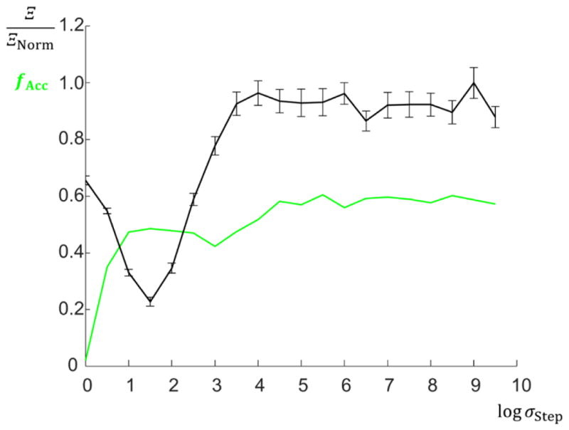
Plot of the acceptance fraction fAcc (green) and average minimum goodness of fit value converged towards with standard uncertainty (black) for several MCMC algorithm runs at different σStep sizes. Uncertainty bars are standard uncertainty for 96 chains. The minimum goodness of fit value converged towards occurred around σStep ≅ 32. Here the objective function Ξ was used and normalized by the number ΞNorm to get the data comparable with the acceptance fractions (i.e. ΞNorm converts the goodness of fit value to arbitrary scaled units; a value of ΞNorm =3578 was used). At large σStep, the algorithm accepts many parameter set moves and thus works poorly. Conversely, at small σStep, the parameter set moves result in almost no acceptance events and the algorithm also works poorly. Thus the medium value of σStep = 32 where Ξ was minimized was used in further MCMC runs.
A.2 DE Algorithm Description and Optimization
For the DE algorithm40, a population set of size psize of P⃗G,C is initiated and the inverse algorithm progresses based on mutation and crossover of these individual parameter sets. psize was set to 96 in this study. Here the indices G and C represent the current generation of the population and individual member index label, respectively. In the algorithm, after each P⃗G,C has a corresponding ΩG,C calculated, all members in the current generation population have their ΩG,C compared against each other and the best value of Ω found thus far. If any individual P⃗G,C yields an ΩG,C value better than the previous best, that P⃗G,C is set as the new best P⃗MF (here MF stands for “most fit”).
Regardless if a new best P⃗MF is found or not, modification of the population for the next generation is accomplished as follows. P⃗MF is kept separate during the mutation and crossover to ensure the best solution is always in the population pool (known as the “Genghis Khan” approach). A mutation step occurs by taking P⃗G,C with the lowest ΩG,C, designated P⃗G,CMF in the current population and differential mixing of two other population members chosen at random are added to the parameter vector modulated by a mutation constant Kmut. In vector form this is simply
| (10) |
where A and B are two random integers in the range from 1 to psize with conditions A ≠ B ≠ CMF. Following the mutation step, a crossover step is implemented going through all NParam elements of each P⃗G,C vector in the population with C ≠ CMF (i.e. C = [1, psize]) and the criterion rand([0,1]) < Kcro is used to determine if the jth parameter of P⃗G,C should be swapped with the jth parameter of P⃗G,CMF. This is analogous to biological meiosis56. In the studies presented Kmut = 0.1 and Kcro = 0.4 based on optimization runs described below. Following the mutation and crossover steps, the new population P⃗G+1,C is generated and the algorithm continues using this new population.
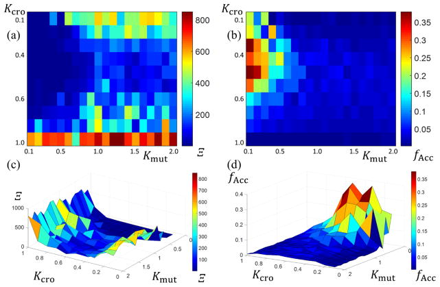
To optimize the DE crossover and mutation parameters, a scan of runs using Kmut ∈ [0.1,2.0] and Kcro ∈ [0.1,1.0] both in steps of 0.1 were performed for a given structure. The goodness of fit Ξ and acceptance fraction fAcc were both calculated for all combinations of Kmut and Kcro examined after NGen =1000 generations. Plots of Ξ and fAcc against the varied parameters are shown in Fig. 8. As seen in the figure, Ξ was minimized around Kmut ≅ 0.1 and Kcro ≅ 0.4 and fAcc was maximal around Kmut ≅ 0.1 and Kcro ≅ 0.5. Unlike the MCMC, fAcc represents only situations where the global goodness of fit decreased since the DE is a true search algorithm and not a stochastic sampler. Thus, the parameters that yield the minimum Ξ values should be expected to correlate well with the values that yield the maximal fAcc which they appear to do. Since the lowest Ξ are desired in the algorithm runs, the combination of parameters Kmut ≅ 0.1 and Kcro ≅ 0.4 were chosen for further runs.
Fig. 8.
Plots of the minimum goodness of fit values Ξ converged towards and the acceptance fraction fAcc for several DE algorithm runs at different Kmut and Kcro values. (a) 2D plot of Ξ versus Kmut and Kcro with bluer colors being lower and redder colors being higher. (b) 2D plot of fAcc versus Kmut and Kcro with bluer colors being lower and redder colors being higher. (c) 3D surface plot of data shown in (a). (d) 3D surface plot of data shown in (b).
A.3 CMAES Algorithm Description
The CMAES algorithm41–43 starts analogously to the DE algorithm with a population set of size psize of P⃗G,C being initiated. The algorithm progresses by calculating a mean weighted parameter vector P⃗G,Mean for each generation that is weighted from the top λmix best individuals in the population with respect to their Ω values. As in the DE algorithm, the indices G and C here again represent the current generation of the population and individual member index label, respectively. Again and analogous to the DE algorithm, each P⃗G,C has a corresponding ΩG,C calculated after intensity simulations are performed with all members in the current generation population having their ΩG,C compared against each other and the best value of Ω found thus far. If any individual P⃗G,C yields an ΩG,C value better than the previous best, that P⃗G,C is set as the new best P⃗MF. Detailed below are all the equations that go into determining the covariance matrix V and mixing equations for the CMAES.
NParam is defined as the number of parameters used in the model that are to be optimized to best fit the data. psize is the population size of parameter sets. pOpt is the lower bound optimal psize needed to get convergence of the CMAES algorithm within generations such that
| (11) |
Using large psize can enhance convergence for a given algorithm run (i.e. lower GOpt) but at the cost of computational time. For consistency between the DE and CMAES algorithms, in this study psize was fixed to 96 for both algorithms which is well above pOpt for any parameter set considered (the largest NParam explored was NParam = 13 → pOpt = 11, much smaller than 96).
λmix is the number of individuals mixed during the CMAES crossover/mutation mixing step. λmix is set equal to λOpt such that
| (12) |
so in this study λmix =48. σ is the parameter coordinate wise standard deviation step size used to scale the mixing of parameter sets for the next generation. σ is set to an initial value of σ1 = 5 and is updated according to the scheme detailed below. σ is reset to σ1 if it surpasses a value σMax which for this study was set as 1020 and the corresponding evolutionary parameters reset to avoid numerical overflow.
| (13) |
ϕC is the crossover probability weight for an individual C with the individuals in the population up to λmix. This is calculated once at the beginning of the algorithm and then remains the same throughout when used in calculating P⃗G,Mean.
| (14) |
λEff is the effective number of individuals mixed in each generation used in calculating several of the evolutionary strategy updating parameters.
G is the current generation number which is increased each generation until reaching a preset value GMax. When psize = pOpt this maximum value should not be larger than
| (15) |
assuming the problem is bound correctly. In practice GMax was set to values ≈ 40000 for consistency between runs, but because an additional criterion checking if Ω < ΩCrit is used to end the algorithm run meaning this GMax is not always reached. During the algorithm, when objective function goodness of fit values are compared, the most fit individual GMF is kept for reference along with the generation that individual was found GMF and the corresponding parameter set P⃗MF.
The following parameters are used in updating the covariance matrix V and step size σ. They are tV, the time constant for the accumulation of V, tσ, the time constant for the accumulation of σ, R1, the rate for the update of the 1st rank update of V, Rλmix, the rate for the update of the rank update of V, and δσ, the damping coefficient for the generational update of σ which is ≈ 1. These parameters remain the same throughout an entire CMAES run.
| (16) |
| (17) |
| (18) |
| (19) |
| (20) |
The following parameters are internal algorithm updating parameters that are updating during every generation. They include P⃗G,V, the parameter evolution path for V, P⃗G,σ, the parameter evolution path for σ, B, the eigenvector matrix of the covariance matrix V initialized as an identity matrix of size NParam by NParam, D, the diagonal eigenvalue matrix of the covariance matrix V again initialized as an identity matrix, and XN, the expectation value constant from of normally distributed random values of length NParam used in the generational update of σ. Thus the covariance matrix is given as
| (21) |
where T is the matrix transpose operator. In updating the parameter evolution paths, the inverse square root of the covariance matrix V−1/2 is a useful quantity to calculate during each step given as
| (22) |
XN is given as
| (23) |
P⃗G,Mean is calculated from ϕC and P⃗G,C where P⃗G,C is sorted with parameter sets in increasing goodness of fit value.
| (24) |
The parameter evolution path vectors during each generation are updated as follows:
| (25) |
| (26) |
where
| (27) |
The covariance matrix for the next generation VG+1 is then given as
| (28) |
where
| (29) |
and σG+1 for the next generation is given as
| (30) |
The population of parameters for the next generation P⃗G+1,C is then given as
| (31) |
where η is a vector of size NParam with random numbers drawn from a normal distribution with standard deviation 1 and the Undiag(*) function outputs the diagonal values of a square matrix as a vector. The values used for B and D in updating P⃗G+1,C are only updated when the following condition is satisfied:
| (32) |
where GE = 0 to start and GE is set to the current G each time B and D are updated. When such an update occurs, the covariance matrix V is updated by the following scheme to ensure the matrix is symmetric.
| (33) |
B and D are then found by solving the eigenvalue problem
| (34) |
Appendix B: Details of Calculating Intensities from the Trapezoid Model
In the trapezoid model system the base intensity (square of the form factor) is given as
| (35) |
where
| (36) |
with Θ =L or R for left and right, respectively, such that the mth trapezoid is defined by the intersection of the four lines
| (37–40) |
In terms of the model parameters, these slopes and intercept parameters are defined such that
| (41) |
| (42) |
and
| (43) |
A general parameter vector for this model will have the following form:
| (44) |
This form would yield 6M+3 independent parameters, but usually this number is reduced by additional constraints placed on a given model for a system. For a single trapezoid, the corner position is generally assumed to be that of the origin (x1, z1)=(0,0) and the SLD usually is assumed to have a fixed value making a single trapezoid model only have 6 independent parameters (3 geometric parameters with 3 intensity scaling parameters). For a column of M trapezoids stacked on top of each other, each trapezoid in the middle of the stack shares widths with the trapezoids above and below them with their positions being fixed by those adjoining trapezoid widths, making the total number of parameters for such a system assuming the SLD to be the same for each trapezoid be NParam = 2M + 4 as there are M + 1 independent widths, M independent heights, and 3 intensity scaling parameters. For a periodic array of c columns of M trapezoids with each column independent of the adjoining column and fixed column widths, the only additional parameter needed to specify each column beyond the first is the position of the lower left corner of the column, giving
| (45) |
More complicated models with various constraints can be made based on these ideas, but for the current manuscript only the kinds mentioned here are investigated.
Appendix C: Parameters and Bounds for the Different Structures
Table 4 through Table 9 list all the simulated structure parameters and the corresponding upper and lower bounds imposed on them during the inverse algorithm runs. Additionally, the expected parameters from the previous experimental study with the bounds used for those runs are listed in Table 10. For Table 10, the lower bounds for the heights were set slightly above 0 to disallow M = 2 or 1 trapezoid solutions (i.e. where a given H would go to 0) but also allow approach of such solutions to be possible in case such solutions were along path trajectories towards the best solutions. The parameter IExp and IBk were calculated based as effective values as the previous study used an additional set of data with qz ≅ 0 nm−1 for a range of qx from near 0 nm−1 to just over 1 nm−1 that was used to rescale the peak intensities during fitting (thus the input values in that study were different, so the values presented here are after rescaling). As a reminder from the main text, SC stands for single column and DC for double column. The width and height parameters generally had a large bound range to ensure decent parameter space coverage with a tighter bound range being imposed on DW and the intensity scaling parameters IExp (IS = 10IExp) and IBk. IBk always had a minimum bound of 0.01 to ensure that the intensities were always greater than 0 so that Ξ did not have singularities (i.e. Ξ → ∞ as ISim → 0).
Table 4.
Target parameters with bounds used for SC M = 1 trapezoid target structure. Units for Wj, Hj, and DW are all in nm.
| SC M =1 | WB | WT | H | DW | IExp | IBk |
|---|---|---|---|---|---|---|
| Parameter Value | 30 | 10 | 15 | 0.5 | −2 | 0.5 |
| Lower Bound | 1 | 1 | 1 | 0 | −5 | 0.01 |
| Upper Bound | 40 | 40 | 40 | 2 | 0 | 1 |
Table 9.
Parameters with bounds used for DC M = 2 trapezoids per column target structure. Units for Wj, Hj, and DW are all in nm.
| DC M = 2 | W11 | W12 | W13 | H11 | H12 | W21 | W22 | W23 | H21 | H22 | DW | IExp | IBk |
|---|---|---|---|---|---|---|---|---|---|---|---|---|---|
| Parameter Value | 15 | 7.5 | 10 | 12.5 | 7.5 | 5 | 10 | 2.5 | 7.5 | 10 | 0.5 | −2 | 0.5 |
| Lower Bound | 1 | 1 | 1 | 1 | 1 | 1 | 1 | 1 | 1 | 1 | 0 | −5 | 0.01 |
| Upper Bound | 40 | 40 | 40 | 40 | 40 | 40 | 40 | 40 | 40 | 40 | 2 | 0 | 1 |
Table 10.
Parameters with bounds used for SC M = 3 trapezoids experimental data structure. Units for Wj, Hj, and DW are all in nm.
| Experiment | W1 | W2 | W3 | W4 | H1 | H2 | H3 | DW | IExp | IBk |
|---|---|---|---|---|---|---|---|---|---|---|
| Parameter Value | 21.83 | 15.13 | 12.89 | 1.92 | 5.74 | 17.57 | 2.93 | 1.26 | −2.22 | 0.49 |
| Lower Bound | 1 | 1 | 1 | 1 | 0.01 | 0.01 | 0.01 | 0 | −5 | 0.01 |
| Upper Bound | 40 | 40 | 40 | 40 | 40 | 40 | 40 | 2 | 0 | 10 |
In addition to the tables showing the parameters and bounds for the different target structure sets, Fig. 9 through Fig. 13 show schematic diagrams of the target structure shape profiles, the calculated target intensity profile ITar(q⃗) as a function of q⃗ = [qx, qz], and the slices from the profiles with Poisson noise added with constant qx values used for parameter optimization by the different algorithms. Poisson noise is a random value proportional to the square root of the number of observed counts, thus the noise added was developed as
Fig. 9.
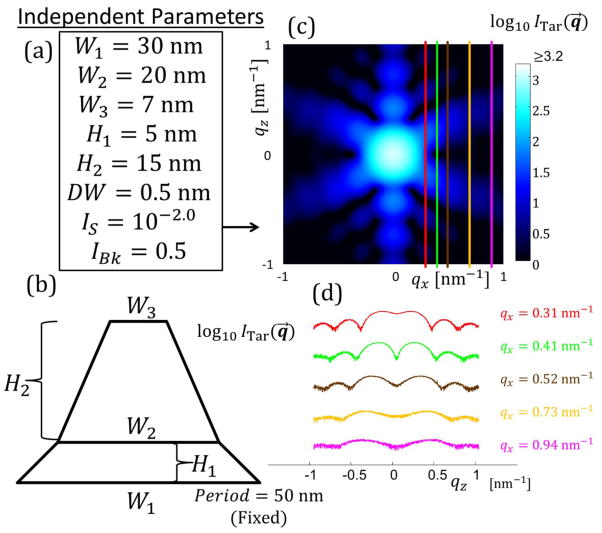
Figure analogous to Figure 3 in the main text for target structure with SC M = 2. Period is fixed as 50 nm. (a) Independent parameters defined for the SC M = 2 structure. (b) Schematic diagram of the shape profile for the SC M = 2 structure. (c) The simulated target structure intensity profile in qz versus qx for a range of [−1:1] nm−1. Intensity is plotted on a log scale with scale shown. Colored lines are constant qx cuts used for parameter optimization with the algorithms corresponding to the intensities shown in (d). (d) Log of target structure intensity slices used for fitting. Scale is arbitrary so the curves all fit on the same plot.
Fig. 13.
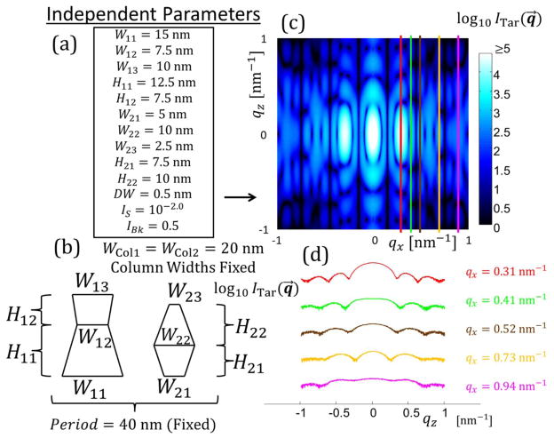
Figure analogous to Figure 3 in the main text for target structure with DC M = 2. Period is fixed as 40 nm. (a) Independent parameters defined for the DC M = 2 structure. (b) Schematic diagram of the shape profile for the DC M = 2 structure. (c) The simulated target structure intensity profile in qz versus qx for a range of [−1:1] nm−1. Intensity is plotted on a log scale with scale shown. Colored lines are constant qx cuts used for parameter optimization with the algorithms corresponding to the intensities shown in (d). (d) Log of target structure intensity slices used for fitting. Scale is arbitrary so the curves all fit on the same plot.
| (46) |
where ICount is the intensity contribution from a single photon scattering event. Since the simulated data is produced at a continuum approximation for the scattering with an analytical Fourier Transform, ICount must be selected independent of the intensity calculation. ICount should be larger than IBk assuming a decent signal-to-noise. Based on the observed experimental values of noise, ICount for the simulated data was chosen to be ICount = 6IBk to get similar noise levels with those observed in experiment. For each simulated intensity, a fixed noise profile was produced for that intensity and used in all runs for that target structure. These figures only show the simulated target structures. For the experimental data, the constant value qx slices were already extracted from the integrated intensity data and their plots can be seen in Fig. 14 where the black curves are the experimental data. An example fit (green) using the CMAES algorithm with the corresponding residuals using M = 3 trapezoids is shown in Fig. 14 as well.
Fig. 14.
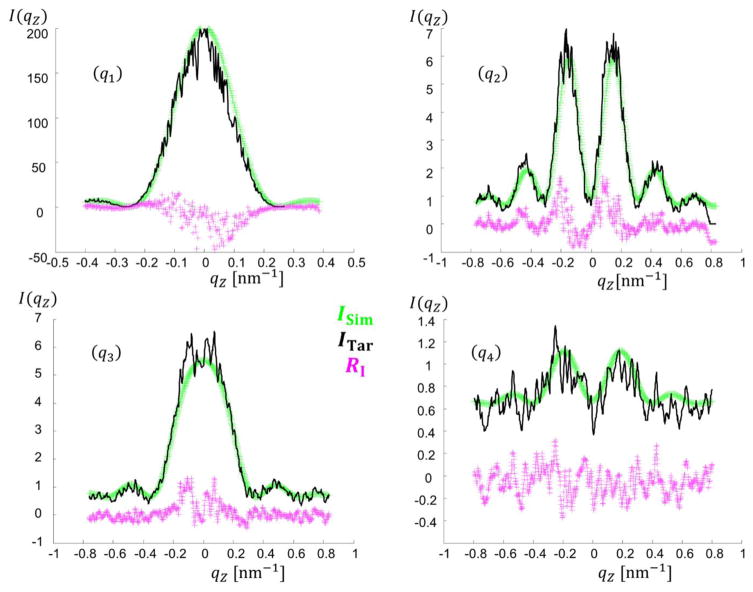
Comparison of plots of the intensity fits found by the CMAES algorithm with Ξ function for the experimental target structure data. The figure shows the experimental data ITar plotted in black, a fit curve ISim plotted in green, and the residuals RI = ITar − ISim between the fit and experimental data plotted in magenta. (q1) Slice 1 qx = 0.223 nm−1. (q2) Slice 2 qx = 0.451 nm−1. (q3) Slice 3 qx =0.677 nm−1. (q4) Slice 4 qx = 0.905 nm−1.
Appendix D: Compiled Results of Different Target Structure Studies
D.1 Simulated Target Structures
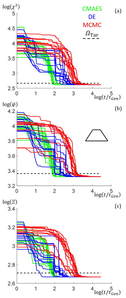
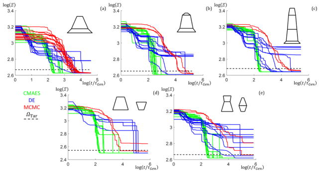
Fig. 15 shows plots for all NRun runs of the SC M = 1 trapezoid target structure goodness of fit values versus normalized time for all three objective functions and three algorithms. Fig. 16 shows plots for all NRun runs of the SC M = 2,3, and 4 structures as well as the DC M = 1 and 2 structures for the Ξ objective function for all three algorithms. In both figures, there are inset images of the target structure. In general, green curves are used for the CMAES, blue curves for DE, and red curves for MCMC. The general trend seen in all cases is that CMAES takes on average about an order of magnitude less time than the DE or MCMC to start rapidly converging towards a minimum goodness of fit value. In terms of actual convergence percentage rate, the CMAES almost always converges within the number of generations tested while DE converges most of the time and MCMC converges more poorly with increasing NParam. Normalized times were chosen for comparison rather than absolute times because different CPU loading conditions affected the absolute times. Thus the normalized times can be compared whatever the speed of the internal CPU clock.
Fig. 15.
Plots of the goodness of fit values for all three algorithms versus the normalized time t/τGen for the SC M = 1 structure. Plots are on log base 10 scale. Inset is a key for which algorithm the colored curves correspond and a schematic of the target structure. The plots have black dashed lines showing the ΩTar values. Plots have all NRuns for the three algorithms of the goodness of fit values versus t/τGen superimposed with different shades of the algorithm distinguishing colors for better clarity. Note there was one case for the DE in (c) that reached ΩTar faster than the CMAES, but the final converged value of Ξ was slightly higher. (a) Ω = χ2. (b) Ω = ψ. (c) Ω = Ξ.
Fig. 16.
Plots of the goodness of fit values for all three algorithms with Ω = Ξ versus the normalized time t/τGen for the multiple trapezoid target structures. Plots are on log base 10 scale. Inset is a key for which algorithm the colored curves correspond and a schematic of the target structure is inset in each corresponding plot. The plots have black dashed lines showing the ΩTar values. Plots have all NRuns for the three algorithms of the goodness of fit values versus t/τGen superimposed. Note that fewer NRuns were performed for the higher NParam structures for the MCMC and DE based on just doing enough to find examples that converged within ΩTar as those runs started to take much longer than t/τGen = 105 to converge on average (corresponding to a few weeks of simulation time). (a) SC M = 2. (b) SC M = 3. (c) SC M = 4. (d) DC M = 1. (e) DC M = 2.
D.2 Experimental Target Structure
Table 11 shows a comparison between the model parameter set solution found in a previous seeded MCMC study with simulations varying the number of trapezoids in the stack model where the CMAES algorithm was used with the Ξ objective function. This is an extended version of Table 2 from the main text. Where no parameter is comparable (because of the number of trapezoids being different) NC is placed in the table for not comparable. In the previous study, one nuance difference to account for when comparing the parameters found in that study is that a fit to a qz ≅ 0 slice of data as a function qx was also used in conjunction with the constant qx peak slices to fit the data requiring the intensities to be rescaled to the maximum peak intensities found. This simply means that the background intensity parameter IBk and scaling exponent IExp cannot be directly compared between the studies, but all geometric shape parameters and the Debye-Waller factor are still directly comparable. The values for the previous study in the table are instead effective parameters found by taking the fit data from the previous study and rescaling the data with the same number of data points.
Table 11.
Comparison of various parameters found for symmetric periodic silicon grating line structure found using experimental data. CMAES with Ξ was used. The parameters presented are the best fit values (corresponding to the lowest goodness of fit values). For the cases of M = 1,2,4, and 5 only the total height HTot and full width at half max height WFWHM were compared since the individual trapezoid components making up the structure in those cases are not comparable (NC).
| Parameter | M = 1 | M = 2 | M = 3 | M = 4 | M = 5 | Previous Study M = 3 |
|---|---|---|---|---|---|---|
| HTot [nm] | 25.66 | 26.65 | 26.55 | 26.97 | 26.73 | 26.24 |
| H1 [nm] | NC | NC | 7.80 | NC | NC | 5.74 |
| H2 [nm] | NC | NC | 16.15 | NC | NC | 17.57 |
| H3 [nm] | NC | NC | 2.59 | NC | NC | 2.93 |
| WFWHM [nm] | 13.55 | 13.85 | 13.87 | 13.92 | 13.97 | 14.19 |
| W1 [nm] | NC | NC | 21.36 | NC | NC | 21.83 |
| W2 [nm] | NC | NC | 14.67 | NC | NC | 15.13 |
| W3 [nm] | NC | NC | 12.30 | NC | NC | 12.89 |
| W4 [nm] | NC | NC | 1.84 | NC | NC | 1.92 |
| DW [nm] | 1.51 | 1.29 | 1.20 | 1.20 | 1.25 | 1.26 |
| IExp | −2.33 | −2.34 | −2.36 | −2.36 | −2.33 | −2.22 |
| IBk | 0.76 | 0.65 | 0.64 | 0.64 | 0.65 | 0.49 |
| Ξ | 0.236 | 0.199 | 0.186 | 0.185 | 0.187 | 0.195 |
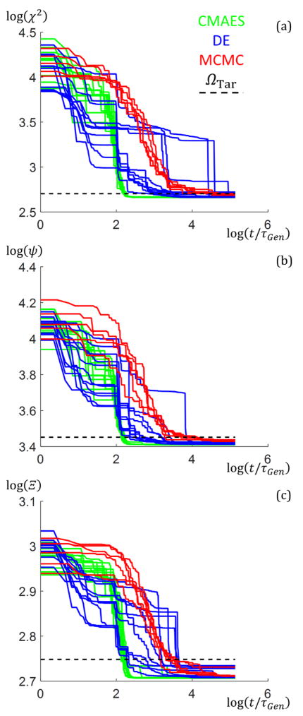
To explore how well the different algorithm and objective function combinations converged to appropriate parameter set solutions for the experimental data set, plots of the goodness of fit values versus t/τGen were made. These plots are shown in Fig. 17 with green curves for the CMAES, blue curves for DE, and red curves for MCMC. These results are from NRun = 11 for the CMAES and DE algorithms and NRun = 5 for the MCMC. Similar trends are seen here that were seen for the simulated target structure data for the trends of when the algorithms start to converge with the CMAES being the best followed by DE and MCMC.
Fig. 17.
Plots of the goodness of fit values for all three algorithms versus the normalized time t/τGen for the M = 3 experimental data set. Plots are on log base 10 scale. Inset is a key for which algorithm the colored curves correspond. The black dashed lines indicates the ΩTar values. Plots have all NRuns for the three algorithms of the goodness of fit values versus t/τGen superimposed. (a) Ω = χ2. (b) Ω = ψ. (c) Ω = Ξ.
Appendix E: List of Abbreviations and Symbols
Abbreviations/Acronyms
- CDSAXS
Critical dimension small angle X-ray scattering
- OCD
Optical critical dimension
- MCMC
Markov chain Monte Carlo
- DE
Differential evolution
- CMAES
Covariance matrix adaptation evolutionary strategy
- SC
Single column
- DC
Double column
Symbols/Variables
- SLD or ρ
Scattering length density
- r⃗
Position vector in real space with coordinates x and z
- NShape
Number of independent parameters describing the shape profile in the models
- NParam
Number of independent parameters (includes NShape and 3 intensity scaling parameters)
- G
Iteration (MCMC) or generation index (DE/CMAES)
- C
Chain number (MCMC) or population individual index (DE/CMAES)
- P⃗
Parameter vector of size NParam for the set of parameters
- κ
Parameter index
- q⃗
Reciprocal space vector with coordinates qx and qz
- I
General intensity variable (subscript distinguishes type)
- ISim
Simulated scattered intensity corresponding to a model parameter set
- ITar
Experimental scattered intensity or target simulated scattered intensity
- Ω
General goodness of fit value
- ΩCrit
Value used as one deciding factor in exiting an inverse algorithm
- P⃗MF
“Most fit” parameter set (i.e. model parameter set that gives the lowest Ω found)
- I0
Absolute square of the form factor (unscaled simulated intensity)
- IS
Multiplicative scaling intensity parameter
- IExp
Logarithm of IS in base 10
- DW
Debye-Waller factor (~interfacial thickness between materials in shape model)
- IBk
Background intensity shifting parameter
- F
General function
- M
Total number of trapezoids used in shape profile model
- m
Index label for a given trapezoid in shape profile model
- WB
Bottom width of a given trapezoid
- WT
Top width of a given trapezoid
- H
Height of a given trapezoid
- Nq
Number of data points used in calculating goodness of fit values (i.e. number of qx and qz coordinates used)
- χ2
Chi squared objective function
- Ξ
Mean absolute error log objective function
- ψ
Mean absolute error objective function
- α
Index for algorithm type (MCMC, DE, or CMAES)
- tConv
Time needed for a given algorithm to converge to within a given goodness of fit value
- t
General time variable
- τGen
Time needed for a single generation or iteration to finish
- GConv
Number of generations needed for a given algorithm to converge within a given goodness of fit value
- τα
Time constant for the average time for a single generation step for a given algorithm α
- ΩTar
Goodness of fit value that needs to be reached to have a solution within desired accuracy
- ΩConv
Theoretical best Ω value possible if exact parameter solution is found
- psize
Number of individual parameter sets used in a given genetic algorithm run (population size in CMAES/DE or number of chains in MCMC)
- NRuns
Number of times an algorithm was used with different initial conditions for the same input data (simulated or experiment)
- WFWHM
-
Full width at half maximum height for a column of trapezoids. Used in comparing the widths of trapezoid stacks of varying number modeling the same data set.
Best Subscript notation indicating a solution has the lowest found goodness of fit
- RI
Residual of the target and simulated intensities
- NChains
Number of chains in MCMC
- rand([n1, n2])
Function whose output is a random number drawn from a uniform distribution with minimum n1 and maximum n2
- ΩMF
Lowest global goodness of fit value found during an inverse algorithm run
- V⃗move
Parameter move vector in MCMC
- B⃗Upper
Upper bound parameter vector
- B⃗Lower
Lower bound parameter vector
- R⃗
Random contribution to V⃗move
- σStep
Step size in MCMC, the parameter move size is inversely proportional to this factor
- fAcc
Fraction of moves that are accepted during an algorithm run under a given criterion
- ΩNorm or ΞNorm
Fidelity value used to normalize goodness of fit value such that it scales with fAcc
- Kmut
Mutation constant in DE
- A and B
Random population index integers in DE mixing scheme
- Kcro
Crossover constant in DE
- λmix
Number of individuals used in mixing in CMAES for making mean parameter set
- P⃗G,Mean
Average parameter vector in CMAES from λmix best parameter sets
- V
Covariance matrix used in CMAES
- pOpt
Lower bound optimal population size necessary for CMAES to converge well
- GOpt
Optimal number of generations needed for CMAES to converge to an acceptable solution when pOpt is used
- λOpt
Optimal mixing size for CMAES algorithm
- σ
Coordinate wise standard deviation step size used in CMAES mixing scheme; Also the shape parameter for the log-normal distribution
- σ1
Initial value of σ in CMAES algorithm
- σMax
Maximum value of σ allowed in CMAES algorithm to avoid numerical overflow
- ϕ
Crossover probability weight (i.e. how much weight a parameter set gives to the mean parameter set) in the CMAES algorithm
- λEff
The effective number of individual parameter sets used in the CMAES mixing scheme based on the values of ϕ
- GMax
Maximum number of generations allowed before algorithm terminates
- MF
Subscript for “most fit” parameter set found within a given inverse algorithm run
- tV
the time constant for the accumulation of V
- tσ
the time constant for the accumulation of σ
- R1
the rate for the update of the 1st rank update of V
- Rλmix
the rate for the update of the rank update of V
- δσ
the damping coefficient for the generational update of σ
- P⃗G,V
the parameter evolution path for V
- P⃗G,σ
the parameter evolution path for σ
- B
the eigenvector matrix of the covariance matrix V
- D
the diagonal eigenvalue matrix of the covariance matrix V
- XN
the expectation value constant
- T
is the matrix transpose operator
- hσ
Constant used in calculating the parameter evolution path vectors
- W
Matrix used in calculating the covariance matrix
- η
Random vector of normally distributed numbers
- Undiag(*)
Function that takes in a square matrix and outputs the diagonal values
- GE
Generation index used in determining if an update to the covariance matrix should be performed
- Θ
Index used for distinguishing the right R and left L sides of a given trapezoid
- BΘ,m
Exponential phase factor used in calculating the scattering of a given trapezoid
- CΘ,m
Exponential difference factor used in calculating the scattering of a given trapezoid
- SΘ,m
Slope of a given trapezoid side
- bΘ,m
Intercept of a given trapezoid side
- c
Number of columns used in trapezoid stack model
- μ
Mean for the log-normal distribution
- PDFΞ
Log-normal probability distribution function
- SF
Scaling factor for scaling log-normal probability distribution function
- PDFΞSF
Rescaled log-normal probability distribution function
- μI
Arithmetic mean of the simulated intensity
- σI
Arithmetic standard deviation of the simulated intensity
- ξ
Poisson distributed background noise added to simulated data
- ICount
Intensity amount contributed by a single photon count in the simulated data
Footnotes
Disclaimer
Certain commercial equipment, instruments, or materials are identified in this paper in order to specify the experimental procedure adequately. Such identification is not intended to imply recommendation or endorsement by the National Institute of Standards and Technology, nor is it intended to imply that the materials or equipment identified are necessarily the best available for the purpose.
References
- 1.The International Technology Roadmap for Semiconductors. 2013 http://www.itrs2.net/itrs-reports.html.
- 2.Sanders DP. Advances in patterning materials for 193 nm immersion lithography. Chem Rev. 2010;110:321–360. doi: 10.1021/cr900244n. [DOI] [PubMed] [Google Scholar]
- 3.Moors R, et al. Extreme-Ultraviolet Specifications: Tradeoffs and Requirements. J Micro/Nanolithogr, MEMS, MOEMS. 2012;11:021102. [Google Scholar]
- 4.Stulen RH, Sweeney DW. Extreme ultraviolet lithography. IEEE J Quantum Electron. 1999;35(5):694–699. doi: 10.1109/3.760315. [DOI] [Google Scholar]
- 5.Gwyn CW, et al. Extreme ultraviolet lithography. J Vac Sci Technol B. 1998;16:3142–3149. doi: 10.1116/1.590453. [DOI] [Google Scholar]
- 6.Benschop J, et al. Extreme ultraviolet lithography: Status and prospects. J Vac Sci Technol B Microelectron Nanom Struct. 2008;26(6):2204–2207. doi: 10.1116/1.3010737. [DOI] [Google Scholar]
- 7.Tomie T. Tin laser-produced plasma as the light source for extreme ultraviolet lithography high-volume manufacturing: history, ideal plasma, present status, and prospects. J Micro/Nanolithography, MEMS MOEMS. 2012;11(2):021109. doi: 10.1117/1.JMM.11.2.021109. [DOI] [Google Scholar]
- 8.Herr DJC. Directed block copolymer self-assembly for nanoelectronics fabrication. J Mater Res. 2011;26:122–139. doi: 10.1557/jmr.2010.74. [DOI] [Google Scholar]
- 9.Kim SO, et al. Epitaxial self-assembly of block copolymers on lithographically defined nanopatterned substrates. Nature. 2003;424:411–414. doi: 10.2494/photopolymer.20.511. [DOI] [PubMed] [Google Scholar]
- 10.Stoykovich MP, et al. Directed assembly of block copolymer blends into nonregular device-oriented structures. Science. 2005;308:1442–1446. doi: 10.1126/science.1111041. [DOI] [PubMed] [Google Scholar]
- 11.Ruiz R, et al. Density multiplication and improved lithography by directed block copolymer assembly. Science. 2008;321:936–939. doi: 10.1126/science.1157626. [DOI] [PubMed] [Google Scholar]
- 12.Bita I, et al. Graphoepitaxy of self-assembled block copolymers on two-dimensional periodic patterned templates. Science. 2008;321:939–943. doi: 10.1126/science.1159352. [DOI] [PubMed] [Google Scholar]
- 13.Yang JKW, et al. Complex self-assembled patterns using sparse commensurate templates with locally varying motifs. Nat Nanotechnol. 2010;5:256–260. doi: 10.1038/nnano.2010.30. [DOI] [PubMed] [Google Scholar]
- 14.Gierak J. Lithography. John Wiley & Sons, Inc; Hoboken, New Jersey: 2013. Focused Ion Beam Direct-Writing; pp. 183–232. [Google Scholar]
- 15.Winston D, et al. Scanning-helium-ion-beam lithography with hydrogen silsesquioxane resist. J Vac Sci Technol B Microelectron Nanom Struct. 2009;27(6):2702–2706. doi: 10.1116/1.3250204. [DOI] [Google Scholar]
- 16.Chawla JS, et al. Patterning challenges in the fabrication of 12 nm half-pitch dual damascene copper ultra low-k interconnects. Proc SPIE. 2014:9054 905404. doi: 10.1117/12.2048599. [DOI] [Google Scholar]
- 17.Van Veenhuizen M, et al. Demonstration of an electrically functional 34 nm metal pitch interconnect in ultralow-k ILD using spacer-based pitch quartering. 2012 IEEE Int. Interconnect Technol. Conf. IITC; 2012; 2012. pp. 1–3. [DOI] [Google Scholar]
- 18.Villarrubia JS, et al. Scanning electron microscope measurement of width and shape of 10nm patterned lines using a JMONSEL-modeled library. Ultramicroscopy. 2015;154:15–28. doi: 10.1016/j.ultramic.2015.01.004. [DOI] [PubMed] [Google Scholar]
- 19.Moore GE. Cramming More Components Onto Integrated Circuits. Proc IEEE. 1998;86:82–85. doi: 10.1109/JPROC.1998.658762. [DOI] [Google Scholar]
- 20.Bencher C, et al. Directed self-assembly defectivity assessment. Part II. Proc SPIE. 2012:8323, 83230N. [Google Scholar]
- 21.Cheng JY, et al. Fabrication of nanostructures with long-range order using block copolymer lithography. Appl Phys Lett. 2002;81(19):3657–3659. [Google Scholar]
- 22.Cheng JY, et al. Templated self-assembly of block copolymers: Top-down helps bottom-up. Adv Mater. 2006;18:2505–2521. doi: 10.1002/adma.200502651. [DOI] [Google Scholar]
- 23.Delgadillo PR, et al. Defect source analysis of directed self-assembly process. J Micro/Nanolithogr, MEMS, MOEMS. 2013;12(3):031112. [Google Scholar]
- 24.Dixit DJ, et al. Metrology for block copolymer directed self-assembly structures using Mueller matrix-based scatterometry. J Micro/Nanolithogr, MEMS, MOEMS. 2015;14(2):021102. [Google Scholar]
- 25.Jones RL, et al. Small angle X-ray scattering for sub-100 nm pattern characterization. Appl Phys Lett. 2003;83(19):4059–4061. doi: 10.1063/1.1622793. [DOI] [Google Scholar]
- 26.Hu T, et al. Small angle X-ray scattering metrology for sidewall angle and cross section of nanometer scale line gratings. J Appl Phys. 2004;96(4):1983–1987. doi: 10.1063/1.1773376. [DOI] [Google Scholar]
- 27.Wang C, et al. Small angle X-ray scattering measurements of lithographic patterns with sidewall roughness from vertical standing waves. Appl Phys Lett. 2007;90(19):1–4. doi: 10.1063/1.2737399. [DOI] [Google Scholar]
- 28.Jones RL, et al. Pattern fidelity in nanoimprinted films using critical dimension small angle X-ray scattering. J Microlithogr Microfabr Microsystems. 2006;5(1):013001. doi: 10.1117/1.2170550. [DOI] [Google Scholar]
- 29.Wang C, et al. Characterization of correlated line edge roughness of nanoscale line gratings using small angle X-ray scattering. J Appl Phys. 2007;102(2):024901. doi: 10.1063/1.2753588. [DOI] [Google Scholar]
- 30.Wang C, et al. Thin Solid Films. 20. Vol. 517. Elsevier B.V; 2009. Small angle X-ray scattering measurements of spatial dependent linewidth in dense nanoline gratings; pp. 5844–5847. [DOI] [Google Scholar]
- 31.Virgili JM, et al. Analysis of order formation in block copolymer thin films using resonant soft X-ray scattering. Macromolecules. 2007;40(6):2092–2099. [Google Scholar]
- 32.Wang C, et al. Defining the nanostructured morphology of triblock copolymers using resonant soft X-ray scattering. Nano Lett. 2011;11(9):3906–3911. doi: 10.1021/nl2020526. [DOI] [PubMed] [Google Scholar]
- 33.Sunday DF, et al. Three-dimensional X-ray metrology for block copolymer lithography line-space patterns. J Micro/Nanolithography, MEMS, MOEMS. 2013;12(3):031103. doi: 10.1117/1.JMM.12.3.031103. [DOI] [Google Scholar]
- 34.Sunday DF, et al. Determination of the Internal Morphology of Nanostructures Patterned by Directed Self Assembly. ACS Nano. 2014;8(8):8426–8437. doi: 10.1021/nn5029289. [DOI] [PubMed] [Google Scholar]
- 35.Sunday DF, et al. Template-polymer commensurability and directed self-assembly block copolymer lithography. J Polym Sci Part B Polym Phys. 2015;53(8):595–603. doi: 10.1002/polb.23675. [DOI] [Google Scholar]
- 36.Liu CC, et al. Chemical Patterns for Directed Self-Assembly of Lamellae-Forming Block Copolymers with Density Multiplication of Features. Macromolecules. 2013;46(4):1415–1424. [Google Scholar]
- 37.Mosegaard K, Sambridge M. Monte Carlo analysis of inverse problems. Inverse Probl. 2002;18(3):R29–R54. [Google Scholar]
- 38.Sarje A, Li XS, Hexemer A. High-Performance Inverse Modeling with Reverse Monte Carlo Simulations. 2014 43rd International Conference on Parallel Processing; 2014. pp. 201–210. [DOI] [Google Scholar]
- 39.Mitchell M. Computers & Mathematics with Applications. 6. Vol. 32. MIT Press; Cambridge, MA: 1996. An introduction to genetic algorithms. [DOI] [Google Scholar]
- 40.Wormington M, et al. Characterization of structures from X-ray scattering data using genetic algorithms. Phil Trans R Sco Lond A. 1999;357(1761):2827–2848. doi: 10.1098/rsta.1999.0469. [DOI] [Google Scholar]
- 41.Hansen N, Ostermeie a. Completely derandomized self-adaptation in evolution strategies. Evol Comput. 2001;9(2):159–195. doi: 10.1162/106365601750190398. [DOI] [PubMed] [Google Scholar]
- 42.Hansen N, Müller S, Koumoutsakos P. Reducing the Time Complexity of the Derandomized Evolution Strategy with Covariance Matrix Adaptation (CMA-ES) Evol Comput. 2003;11(1):1–18. doi: 10.1162/106365603321828970. [DOI] [PubMed] [Google Scholar]
- 43.Hansen N, Kern S. Evaluating the CMA Evolution Strategy on Multimodal Test Functions. Proc. 8th Int. Conf. Parallel Probl. Solving from Nat. - PPSN VIII; 2004. pp. 282–291. [DOI] [Google Scholar]
- 44.Hannon AF, et al. Inverse design of topographical templates for directed self-assembly of block copolymers. ACS Macro Lett. 2013;2(3):251–255. doi: 10.1021/mz400038b. [DOI] [PubMed] [Google Scholar]
- 45.Hannon AF, et al. Optimizing topographical templates for directed self-assembly of block copolymers via inverse design simulations. Nano Lett. 2014;14:318–325. doi: 10.1021/nl404067s. [DOI] [PubMed] [Google Scholar]
- 46.Qin J, et al. Evolutionary pattern design for copolymer directed self-assembly. Soft Matter. 2013;9:11467–11472. doi: 10.1039/c3sm51971f. [DOI] [Google Scholar]
- 47.Khaira GS, et al. Evolutionary Optimization of Directed Self-Assembly of Triblock Copolymers on Chemically Patterned Substrates. ACS Macro Lett. 2014;3:747–752. doi: 10.1021/mz5002349. [DOI] [PubMed] [Google Scholar]
- 48.Ulyanenkov A, Omote K, Harada J. Genetic algorithm: Refinement of X-ray reflectivity data from multilayers and thin films. Phys B Condens Matter. 2000;283(1–3):237–241. doi: 10.1016/S0921-4526(99)01972-9. [DOI] [Google Scholar]
- 49.Fernandes VR, et al. Multi-objective genetic algorithm applied to spectroscopic ellipsometry of organic-inorganic hybrid planar waveguides. Opt Express. 2010;18(16):16580–16586. doi: 10.1364/OE.18.016580. [DOI] [PubMed] [Google Scholar]
- 50.Kudla A. Application of the genetic algorithms in spectroscopic ellipsometry. Thin Solid Films. 2004;455:804–808. [Google Scholar]
- 51.Raymond C. Overview of Scatterometry Applications in High Volume Silicon Manufacturing. AIP Conf Proc. 2005;788:394–402. [Google Scholar]
- 52.Boschetti F, Dentith MC, List RD. Inversion of seismic refraction data using genetic algorithms. Geophysics. 1996;61(6):1715–1727. doi: 10.1190/1.1444089. [DOI] [Google Scholar]
- 53.Aleardi M. Seismic velocity estimation from well log data with genetic algorithms in comparison to neural networks and multilinear approaches. J Appl Geophys. 2015;117:13–22. [Google Scholar]
- 54.Sivia DS, Skilling J. Data Analysis: A Bayesian Tutorial. 2. Oxford University Press; Oxford, UK: 2006. [Google Scholar]
- 55.Marquardt DW. An algorithm for least-squares estimation of nonlinear parameters. J Soc Ind Appl Math. 1963;11(2):431–441. [Google Scholar]
- 56.Bernstein H, Bernstein C. Evolutionary origin of recombination during meiosis. Bioscience. 2010;60(7):498–505. [Google Scholar]


