

Abstract
When crawling on a flat substrate, living cells exert forces on it via adhesive contacts, enabling them to build up tension within their cytoskeleton and to change shape. The measurement of these forces has been made possible by traction force microscopy (TFM), a technique which has allowed us to obtain time-resolved traction force maps during cell migration. This cell ‘footprint’ is, however, not sufficient to understand the details of the mechanics of migration, that is how cytoskeletal elements (respectively, adhesion complexes) are put under tension and reinforce or deform (respectively, mature and/or unbind) as a result. In a recent paper, we have validated a rheological model of actomyosin linking tension, deformation and myosin activity. Here, we complement this model with tentative models of the mechanics of adhesion and explore how closely these models can predict the traction forces that we recover from experimental measurements during cell migration. The resulting mathematical problem is a PDE set on the experimentally observed domain, which we solve using a finite-element approach. The four parameters of the model can then be adjusted by comparison with experimental results on a single frame of an experiment, and then used to test the predictive power of the model for following frames and other experiments. It is found that the basic pattern of traction forces is robustly predicted by the model and fixed parameters as a function of current geometry only.
Keywords: cell migration, cell adhesion, cytoskeleton, emergent material, finite elements, modelling
1. Introduction
During immunoresponse and cancer metastasis formation, cells crawl on the blood vessel wall [1]. This type of cell motion has been reproduced in vitro [2] and has been the subject of many modelling studies [3–5].
As inertial effects and body forces are vanishingly small in this process, all forces are instantaneously balanced in the system and, in particular, the resultant of the traction forces that the cell exerts on its environment has to be zero. The motion of the crawling cell is thus necessarily driven by its deformation, as the cell changes shape both by growth and shrinkage due to (de)polymerization at its leading edges [6,7] and simultaneously as actin cytoskeleton undergoes a persistent centripetal deformation, called retrograde flow [8–10]. To result in a net displacement of the cell with respect to its surroundings, forces need to be transmitted to it. Although fluid drag and non-specific interactions with the solid substrate are present, most of the stress is transmitted via specific adhesion interaction between ligands present on the surface of the substrate and transmembrane receptors which are bound to the actin cytoskeleton [11].
The mechanical models attempting to explain cell migration from the dynamics of its microstructure are thus focusing on the dynamics of actomyosin and adhesion complexes [12]. Important modelling efforts have been made to understand the initiation and maintenance of motility [13–17]. These works are using the simple and stable shape of keratocyte cells, or a one-dimensional (1D) simplification. While this allows for a fine understanding of possible detailed mechanisms of motility and is based on the same mechanisms of actin (de)polymerization and myosin-driven retrograde flow, the migration of keratocyte does not present the cycle of events observed in most other cell types during migration [18]. Moreover, although these models are shown to fit experimental results, in general, they have not yet been exploited in a systematic manner. Indeed, quantitative prediction of cell dynamics and exerted forces is only at its beginning [19–21]. Whereas fitting models remains necessary to acquire a minimal set of parameters from a subset of the experiments available in all cases, these recent papers are additionally predictive of other experimental conditions for which no further adjustment is done.
Here we combine the prediction of a simple yet quantitatively validated rheological model of actomyosin [19] with a nonlinear model of cell adhesion adapted from [16] and simulate it on the actual geometry of cells tracked while crawling. Monitoring the deformation of the substrate during the experiment [22] and a traction force microscopy (TFM) method [23–27] allow us to compute independently the traction forces that the cell exerts on the substrate, to which the predicted traction fields can be compared. The number of adjustable parameters is reduced to a minimum (two for the linear model, four for the nonlinear adhesion model) and the robustness of the parameter choice is assessed in a systematic way. The preditive capability of the model is tested over different cell migration events and cell types.
Experimental observations in the literature give consistent pictures of two different scales: the microscopic scale, at which the dynamics of the relevant molecules are well described (actin, actin-binding molecules and adhesion molecules), and the mesoscopic scale of the cell itself. Our approach is to write a mechanical model based on the microscale knowledge, and to investigate how these microscale dynamics yield the emergent mesoscale behaviours that are observed. In a previous paper [19], we have successfully used this type of approach and validated quantitatively at the mesoscale a rheological constitutive law based on a microscale model of actomyosin dynamics.
However, the set-up used in that work did not require a precise model of the mechanics of cell adhesion, whereas this is needed here in order to address cell crawling. Cell adhesion models of graded complexity have been introduced by many authors [16,28,29]. Our numerical resolution procedure and quantitative comparison with experimental data allow us to investigate which of these models match best the observations.
2. Mesoscale experimental observations
We observe cancer cells from two different cancer cell lines (T24 and RT112 cell lines) which are crawling on a relatively stiff gel, E = 10 kPa. Our experimental observations, traction force recovery and the relevant other observations in the literature are described briefly in appendix A(a) and A(b), and at length in [27]. Here we summarize only some salliant features that will need to be accounted for by the model predictions.
When plated on the gel, T24 cells assume an elongated and digitated shape, while RT112 cells have a rounded shape (figure 1). For both lines, as well as in all other observations in the literature, the traction forces they exert are minimal close to their geometric centre and increases distally (close to the cell edge). The tractions are oriented approximately along the normal to the cell edge, pointing inwards (figure 1c). The rate of increase of traction force along an imaginary line from cell centroid to cell edge is greater when the cell edge is close to centroid, but the intensity of traction goes generally to much larger values close to the part of cell edges which are more distal (farther away from centroid). In many instances, the maxima of the traction field are not situated right at the cell edge but somewhat proximal (inwards) from it, and tractions can be vanishingly small at the edge. In what follows, we will attempt to link these observations with both the phenomenology of adhesion complexes (as done, e.g. in [30]) and with the mechanics of the cytoskeleton.
Figure 1.

Migration of epithelial cancer cells on a 10 kPa substrate. (a) T24 cell line, (b) RT112 cell line. (c) Traction field recorded at selected instants for both cells. (Online version in colour.)
3. Microscale-based mechanical model
It is well established experimentally that the mechanical properties of crawling cells are controlled by their actin structures and the proteins that bind to actin [2]. Although other cytoskeletal components have a smaller contribution in the mechanical balance, we will neglect them in what follows. Above a timescale between 0.1 and 10 s, the pressure in the cytosol equilibrates [31] and the poroelastic behaviour of the cell becomes negligible. Thus, the variable of interest is the stress tensor σ3D in the actin meshwork (and its strain and rate-of-strain tensors ɛ3D and  , see table 1 for a list of model variables and parameters) at any position in the cell. In the absence of inertia and at sufficiently long timescale, the force balance is written as
where F are bulk forces, discussed below. This internal stress of the actin needs to be balanced at the boundaries of the actin meshwork: thus the actin stress acting at boundaries where adhesion molecules are present is equal to the stress T that these exert on the environment at its boundaries.
Table 1.
Parameters and variables reference list.
| notation | meaning, measured or calculated value |
|---|---|
| α, β | any index among x and y |

|
rate-of-strain tensor |
| κ | 2D Lamé's first coefficient |
| no experimental data | |
| Ω3D | space occupied by cell |
| Ωc | projection of Ω3D on plane (x, y) |

|
same, specifying frame number i |
| Ω | field of view containing Ωc |
| τα | relaxation time of actomyosin |
 [19] [19] | |
| cf | effective friction coefficient |

|
friction coefficient where 
|

|
friction coefficient where 
|
| D | typical diameter of cell |
| D = 40–100 µm in experiments | |
| distances non-dimensionalized by D = 50 µm | |
| G | 2D shear modulus |
| h | height of cell |
 , , 
| |
| n | external normal to Ωc in (x, y) plane |
| T | characteristic time of actomyosin retrograde flow |
| T = 103–104 s [19] | |
| non-dimensional model parameters | |
| λ | second viscosity, λ = κ/G |
| taken equal to 1 (arbitrary) | |
| σa = σaI | myosin-generated 2D pre-stress [19] |
| non-dimensionalized by ταG/T = 5 kPa µm from experiments | |
| found to be of the order of 30, i.e. 150 kPa µm | |
| ζ | velocity-dependent friction coefficient |
non-dimensionalized by 
| |
| ζ0 | friction coefficient ζ where 
|
| found to be of the order of 20, i.e. 200 kPa s µm−1. | |
| ζ1 | friction coefficient, where 
|
| found to vary around 5, i.e. 50 kPa s µm−1 | |
| v* | critical velocity (phenomenological parameter) |
| found to vary around 0.1, i.e. 10−3 µm s−1 | |
| De | Deborah number |
 from experiments from experiments | |
| taken from 0 to 1 in 1D solutions, 0 in 2D simulations | |
| non-dimensional model unknowns | |
| σ | 2D stress tensor |
| non-dimensionalized by ταG/T = 5 kPa µm from experiments | |
| v | field of actomyosin velocity in plane (x, y) |
non-dimensionalized by 
| |
| T | field of traction |
| non-dimensionalized by ταG/(TD) = 100 Pa from experiments | |
As the actin flows, its density ρ will evolve. However, there is strong experimental evidence that the density of actin is tightly regulated by filament nucleators and various molecules favouring growth or shrinkage of actin filaments [32]. Denoting by  the target density field of this regulation, and assuming that it has a characteristic time τρ, we can describe this with an advection–reaction equation:
where v3D is the velocity of actin. In what follows, we will assume  , where D is the cell diameter, which leads to the solution of the above equation
  , a uniform constant. This is supported by fluorescent speckle microscopy [33] and indeed, although there are visible local variations in the actin density on fluorescence images, the distribution of fluorescence intensity is well peaked and has a standard deviation of less than 50%.
When adhering on a substrate of sufficiently large stiffness [34], cells spread until their projected surface  has a diameter D of the order 40 (RT112) to 100 µm (T24), and present a flat structure called the lamella [33] whose height is typically less than a few micrometres, and a dome-like structure referred to as the actin-cap, under which the nucleus is located, which has a height of 5–10 µm [35]. In this work, we will consider that this aspect ratio is sufficiently small to justify a two-dimensional (2D) approach in which the cell is treated as a thin layer of thickness h subject to tangential surface tractions T and bulk forces F only, but it should be borne in mind that this is only a first approximation. In this context, we will also consider that the variations of h are small. This geometric setting constrains some components of the 3D stress tensor σ3D: we have
  and
and  for
for  [36] (figure 2e) which allows to rewrite the problem in terms of a 2D stress tensor, with components
  , and write the 2D force balance as
See figure 2a,b for a sketch of this mechanical balance. In practice, F = 0 as bulk forces such as gravity are negligible and no external force is applied on the cell. At the cell edge  (which is noted experimentally to correspond to the contact line of the cell with the substrate,
  ), there is no specific line force so the stress tensor σ along this boundary must vanish (figure 2b)
| 3.1 |
The stress tensor σ needs then to be related with the deformations by a constitutive law. As most of the intracellular stress is borne by the actin meshwork, it is the deformation of actin which is relevant to study in a first approximation. We have derived and validated such a rheology for the actomyosin cortex in [19], by taking into account the dynamics of cross-linkers that bind to actin and the input of mechanical energy by the myosin motor molecules. The dynamics of cross-linkers is modelled by a single constant residence time, τα, which was found to be of the order of 103 s for two cell types (fibroblasts and myoblasts). The myosin molecular motors, which are among the cross-links that bind and unbind, are in addition responsible for a supplementary term in the constitutive relation, which reads as a pre-stress  , where αmyo is the fraction of cross-linkers which are myosin filaments, and effectuate a power-stroke of step length
  at frequency 1/τmyo. G is the elastic modulus of the cross-linked actin network and β is inversely proportional to its Kuhn length. In [37], we have shown that the fluorescence intensity of labelled myosin molecules could provide a proxy for the local variations of αmyo; however here, in the absence of measurements for most of individual terms in σa, we will treat it as a constant globally, as was done successfully in [19]. For the sake of simplicity, we will also assume that the actin filaments are isotropically distributed in the plane parallel to the substrate, and define the pre-stress tensor
  . With these assumptions, the constitutive equation writes
| 3.2 |
where  is the rate-of-strain tensor,
  the objective upper-convected time-derivative of the stress tensor σ and κ is Lamé's first coefficient. The group
  has the dimension of a viscosity and this term corresponds to the energy dissipated in (slowly) deforming the actomyosin network [38] in an irreversible manner due to cross-linker unbinding [19]. This balance of stresses and the deformations linked with the viscous stresses are described in figure 2c,d. This rheology is in line with early models of actomyosin [39] and active gels models [40]. We do not supplement this contractile liquid behaviour with an elastic resistance term of the cell, contrarily to what is done in mechanosensing [41,42] and migration models [17]. Other models have also considered the same rheology for cell migration, with an additional inertial term used for numerical stabilization [4].
Figure 2.

Mechanical balance and dynamics of the cell. (a) Three-dimensional mechanical balance. (b) Two-dimensional mechanical balance (top view). The 2D stress tensor (components σxx, σxy = σyx, σyy) and the traction field T are defined over the cell domain Ωc. The stress vanishes along  , σn = 0. (c) Stresses applied to a 2D element: the stress σ of the neighbouring actin elements is felt at the boundaries, the reaction force of the substrate for traction T is distributed over the area of the element, and σa is the pre-stress created by myosin contractility. Neglecting the fast elastic response for simplicity, the resultant of these stresses must be balanced by viscous stresses, equal to
  . (d) Rate-of-strain
  of a 2D element and associated velocity field v. (e) The traction force field T, assumed tangential, is equal and opposite to the shear components
  of σ3D at the contact surface. (f) The binding of transmembrane adhesion complexes (red symbols) to actin is highly dynamic, resulting in an effective viscous friction law for T. (g) The dependence of the friction number
  on the local actin speed |v| is modelled in different ways: dashed red line, constant by piece (for 1D analytical model), solid blue line, decreasing hyperbolic tangent (for comparison with [16] and numerical simulations), dotted red line, decreasing exponential (in good agreement with experimental measurements [30]).
Finally, a rheological law must be proposed for the relationship between the traction forces T and the relative displacement between the substrate and the cell [3,36]. Here again, the relevant structure to define a displacement within the cell is the actin meshwork, which is mechanically bound to adhesion molecules. In a first approximation, we assume that the substrate displacement rate is small compared with the velocity of the actin within the cell,  . This hypothesis will need to be questioned in future work, as experiments show that substrate displacement rates are of the order of 10−3 µm s−1, comparable with the speed of retrograde flow. With this simplifying hypothesis, the relative speed of actin with respect to the substrate is the velocity v of actin in the laboratory reference frame and
  . On the ground that adhesion complexes are very dynamic [11], we can expect a friction-like behaviour (figure 2f)
| 3.3 |
where cf may depend on the velocity |v|. This is assumed in many modelling approaches, including [17,28] where cf is taken constant, and in [43] where position-dependent and dissymmetric adhesion is implemented.
However, experiments show that although local traction force and actin velocity are positively correlated on the whole, above some critical velocity, the traction forces drop by several folds [16,30], indicating that cf is not uniformly constant. The causes of the drop in cf are only speculated, as locations with a lower cf share three related characteristics: the actin flow speed is above a threshold v* which seems to be a cell-type specificity ( in fast-migrating keratocytes [16],
  in mammalian Ptk1 epithelial cells [30]), they are located more distally and adhesion complexes there are less mature [30]. Barnhart et al. [16] propose a differential equation that implements these different effects. Note that the precise role of the different terms in this model has not been experimentally tested so far, and Barnhart et al. [16] claim that a simple algebraic relation as exemplified in figure 2g captures the phenomenology. We choose to use the same algebraic relationship as they do,
  , in order to test whether it is able to produce a fair quantitative prediction of traction stresses.
The modelling discussed so far describes only a (dynamic) mechanical equilibrium, giving a snapshot of the force balance and rate of strain of the actin network. It is not in the scope of this paper to try to predict the subsequent dynamics of the cell, which would require to describe also processes such as actin polymerization-based protrusion [2], or to provide some other more or less explicit dissymetrization of the dynamics. Indeed, in order to obtain a persisting motility, models require a more or less explicit dissymetrization either of the actin treadmilling [28,44], of the myosin contractility σa [16,45] or of the curvature of a contractile structure [15]. In one dimension, the need for such an effect can be proved [46]. Here, we show that the traction forces observed in cells are not dominated by this dissymetrical component, since an entirely symmetrical model allows us to give good predictions of the observations. Further refinement of the model and comparison with the experiments, and new experiments tracking explicitely myosin and adhesion molecules will be needed in the future to address this question.
Two length scales appear in the problem: one, the cell diameter D, is directly observable but depends on cell type and fluctuates during migration, the other is a friction length  . The speed of retrograde flow vt measured at the leading edge in [47] and calculated from the modelling of cell-scale experiments in [19] is convenient to scale the rate of deformation of the cytoskeleton: as vt is of the order 10−3–10−2 µm s−1, and the cell radius of the order of tens of micrometres, a characteristic time is T = 103–104 s. The other timescale in the problem is the relaxation time τα, in [19], we find
  : thus the visco-elastic term
  can be expected to be of a lower magnitude than σ in the consitutive equation (3.2), although it is not a priori negligible. If we choose to scale stresses with
  , the non-dimensional model is
| 3.4a |
| 3.4b |
where we introduce the friction non-dimensional number  , based on a friction length
 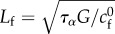 for some reference friction coefficient
  and the Deborah number
  .
.
4. Results
4.1. One-dimensional model predictions
In order to reach a good understanding of the mechanical balance that the model describes, we first study it in 1D. The cell is assumed to occupy a segment of the real axis, and as we do not introduce explicitly a dissymetry, our model will predict a solution which is symmetrical with respect to the midpoint of this segment. This simplistic setting thus corresponds to cells which are not migrating or polarized. The non-dimensional equations for the permanent regime on the domain (−1,1) are
| 4.1a |
| 4.1b |
| 4.1c |
where we have slightly changed the non-dimensionalization, using  instead of G when scaling stresses. Note the nonlinear coupling term
  , which arises from the upper-convected objective derivative of the stress tensor, in [36,43], an analogue 1D model with the co-rotational derivative is proposed.
Analytical solutions can be obtained in the case De = 0, and numerical approximations otherwise, the solution procedure is described in the electronic supplementary material, text A. An example of dynamical mechanical equilibrium is shown in figure 3b, for the case of a uniform friction number ζ = ζ0 and a vanishing relaxation time De = 0. A centripetal flow
corresponding to the retrograde flow, is observed [36]. It is maximal close to the cell edge, and its intensity is proportional to the myosin activity σa, consistent with experiments [33,47]. The traction force density T is by hypothesis directly proportional to the retrograde flow here, and thus centripetal and maximal close to cell edges too. The stress in the actomyosin vanishes at the cell edge, which corresponds to our imposed boundary condition, and is maximal at the cell centre in proportion with myosin activity σa:
It is thus myosin activity that puts the actin network under tension, a tension which is balanced at the cell edges by friction via the friction number ζ. If ζ is large, the tension is constant in most of the domain and balanced by traction forces in a narrow zone close to the edge (figure 3b).
Figure 3.

One-dimensional model and results. (a) Schematic of the relevant structures for cell mechanics and of the variables of interest. We define the stress tensor σ and the velocity v of the filamentous actin network at every point of the 1D domain corresponding to the cell. The cell interacts with its environment mostly through specific adhesion complexes, which link the intracellular actin network with the substrate, we name T the traction forces that actin exerts on the substrate via these adhesions. The relationship between stress tensor σ and velocity v is modelled by the rheological constitutive law (3.4a); the relationship between the relative velocity of actin with respect to the substrate v and the traction force field T is given by the friction model (3.3). (b) Analytical result of system (4.1) with De = 0, σa = 1 and a uniform friction with friction length Lf = 0.1 D. The stress tensor σ (reduced to its xx component), velocity v and traction field T are represented by their magnitude (respectively, green, black and red curves) and vector or tensor representation (green, black and red arrows or double-pointing arrows). The stress is mostly constant and positive in the cell lamella and body, corresponding to a tension, which is balanced by centripetal traction forces concentrated at the periphery. The tension gives rise to a deformation rate of the actin, resulting in the retrograde flow. (c) Same as (b) but with Lf = 0.3 D. The weaker friction number leads to a wider peripheral zone of large tractions, but also to build up a lower tensile stress σ, as the actin yields more and flows at higher velocity. (d) Same as (c) but with a nonuniform friction number, equation (4.2), ζ1/ζ0 = 0.16 and v* = 0.26.
In the case when De = 0.1, which corresponds to our estimates for experimental cases, the solution differs little from the De = 0 solution (electronic supplementary material, figure S3a). For De ≥ 1, a quantitative deviation can be appreciated (electronic supplementary material, figure S3b), but there is no strong qualitative difference. We will thus focus on the case De = 0 from this point, as this allows analytical 1D calculations and less involved numerical simulations in 2D (although the visco-elastic case De > 0 can be treated, see e.g. [48] using the approach in [49]).
We then turn to the case of a nonlinear friction number ζ = ζ(|v|), in order to allow analytical resolution we take a piecewise constant function (figure 2g):
| 4.2 |
with ζ1 < ζ0 consistently with observations [16,30]. In figure 3d, we see that this results in a more uniform retrograde flow close to the cell edge, which is due to the fact that there is less of a gradient of tension there, due to a lower local friction. Because of the low friction number locally, traction is low close to the cell edge, which is the phenomenology that we wanted to reproduce.
Numerically, we can solve with  (figure 2g) which is closer to the experimental observations [30], this gives a smoother behaviour but no essential qualitative difference.
4.2. Prediction of the traction field of a motile cell
Turning now to a 2D approach, we ask whether for a given cell shape, the above model can predict the traction pattern that we measure by TFM, as in figure 1. Starting from the data of Ωc for a typical experimental result, we calculate using a finite-element approach (see appendix A(c)) the traction field for a linear friction law (cf independent of v) and a choice of the two parameters: friction number ζ0 and myosin contractility σa. As in 1D, the magnitude of the stress, retrograde flow and traction forces are in direct proportion to σa (see the electronic supplementary material, text B.2), while changes in ζ0 will modify the pattern of retrograde flow and traction forces. In consequence, we can find explicitly an optimal value for σa for a given value of ζ0, and optimize for this parameter in order to get the best fitting approximation of the experimental traction field (figure 4a). The relative error on the traction vectors is  , that is, the error vectors
  have a magnitude 0.73 times the experimental vectors Texp in L2 norm. This can be considered a fair result for a two-parameter fit of a vector field with rich features. Indeed, the experimental traction field at this instant indicates that there is probably no mature adhesion under the protrusion visible on the left hand side, since the traction field decreases dramatically there. This feature cannot be described by this first model where the friction number is taken to be a homogeneous constant, thus limiting the possibility to approximate the experimental observations. The relative error on the intensity of traction is
  , thus the error is shared between a mismatch between experimental and predicted magnitude of traction field, and some misalignment of the experimental and predicted traction vectors. The optimal parameters are found to be
  , which implies a friction length of the order of 10 µm, and
  . Using the numerical value of parameters τα and vt that we have obtained in [19] for two other cell types, this would imply that the myosin pre-stress σa is about three times the zero-shear elastic modulus G of the actomyosin meshwork, in [19] the same ratio was found to be 4.3.
Figure 4.

Two-dimensional linear model predictions compared to experimental results. Throughout this figure, the friction number ζ is a uniform constant equal to  . The only two free parameters of the model are adjusted to
  = 19.4 and
  = 27.7 (both non-dimensional) so as to match best experimental traction field Texp in panel (a); they are used to predict traction fields for observed cell shapes Ωci in panels (b–e). (a) Comparison of traction field predicted by the model (red arrows) and calculated from experimental observations (blue arrows) at the initial instant t = 0 of a migration experiment of a T24 cell. In the uropod (right), a good agreement is found with an alignment mismatch ranging from close to 0 up to nearly 90 degrees in a small subregion. In the slender part linking the uropod with the cell body, intensity of traction is low in predictions and experiment. Around the cell body (thicker part where the nucleus is located), the magnitude of traction is rather well predicted, and the alignment mismatch ranges from 0 to 45 degrees. The model predicts the observed tractions oriented from nucleus area towards the lamella at the cell front with a very good alignment and magnitude. Finally, in the lamella region (left), the global centripetal traction field is predicted, although the location of the maximal traction is not predicted: indeed, close to the leading edge, we note experimentally low tractions which cannot be reproduced by the linear model, and which may be due to unmature or rupturing adhesions. (b) Comparison of traction field predicted by the model (red arrows) and calculated from experimental observations (blue arrows) at the initial instant of a migration experiment of an RT112 cell. No parameter adjustment. The RT112 morphology is much simpler, and the model predicts a centripetal traction field which globally agrees with observations. The same shortcomings of the model as for the lamella region in T24 cells (a) are noted. (c) Comparison of the field of traction intensity across a full migration cycle as predicted by the model (left) and calculated from experimental observations (right) for the T24 cell in panel (a). Magnitudes are given in Pascals. From top to bottom, a subsample of the experimentally recorded steps is presented, every 6 min (
 min). No parameter adjustment was done for t > 0. Although the maximum traction observed experimentally is not always right at the leading edge, the global pattern and size of high-traction regions are predicted by the model throughout the migration cycle, across variations in cell area, aspect ratio and orientation. (d) Same for the RT112 cell in panel (b) at t = 0. See electronic supplementary material, figure S5 for t > 0. Magnitudes are given in Pascals, no parameter adjustment. (e) Relative error of the predicted tractions compared to experiments for the n = 21 instants at which a frame was recorded in experiments. Relative error on traction vectors
  , and on intensity of traction
  is presented for the three experiments on cell types T24 and RT112. No parameter adjustment was done for individual experiments and instants,
  and
and  are used throughout the n = 66 frames.
During the experiments, cell position and shape  and traction forces
  were acquired at several instants ti 2 min apart. We now ask whether our model and the parameters
  and
and  can, for these different cell shapes
  , predict the traction forces
  without further parameter adjustment. We find that for the 21 frames of the experimental results, the relative error on traction vectors ranges from 0.53 to a maximum of 0.75, with a median of 0.60, which indicates that the parameters that where optimal for one instant give as good results for other frames (figure 4c,e) even though the aspect ratio of the cell changes by a factor 2 depending on the stage of the migration process. The relative error on traction intensities ranges from 0.48 to 0.61, with a median of 0.57.
Thus, the parameters describing the mechanical behaviour of a migrating T24 cell are approximately conserved over more than half an hour during crawling. We then tested whether these parameters could also predict a good approximation of the traction stresses exerted by another cell of the same type in the same conditions. The comparison of the predictions of the model, using the same values  and
and  as for the first T24 cell, are shown in the electronic supplementary material, figure S4, the error of the predicted traction field varies in the same range as for the first cell (figure 4e).
Next, we considered the other cell type that was studied experimentally (RT112 cells). These cells spread to a much lower area on the substrate and maintain a rounded shape which evolves little in the course of migration. Although these characteristics are reminiscent of amoeboid migration, RT112 crawl at smaller speed and exert larger tractions than T24 [27]. All these characteristics make RT112 cells very different from T24, and we asked whether this is due to a different mechanical balance altogether, or different quantitative importance of several effects. However, when applying the same mechanical model as above with the parameters  and
and  , a fair approximation of the traction field obtained experimentally is recovered (figure 4b,d). This is equally true for the all 20 frames of this RT112 experiment (electronic supplementary material, figure S5) the median of the relative error on traction vectors is 0.63 and its range from 0.57 to 0.71, and traction intensities have a median error of 0.52 and a range from 0.43 to 0.57 (figure 4e).
For both RT112 and T24 cell types, experimental results show that the traction field maxima are generally not located quite at the cell edge, but somewhat proximal from it. As seen in the 1D calculations (figure 3d), this is compatible with the model provided that there is a switch from a large friction number ζ0 to a lower one ζ1 above some relative velocity v*. For an appropriate choice of these parameters, the model prediction is improved (figure 5a). The median error on traction vectors drops from 0.73 to 0.61 and the one on the traction intensity from 0.59 to 0.48, the better agreement is not only in a large part due to a better match in magnitude of the traction in the protrusion at the cell front, but also in a better match of the directionality of tractions in this area.
Figure 5.

Two-dimensional nonlinear model predictions compared to experimental results. Two of the free parameters of the model are kept equal to ζ0* = 19.4 and  = 27.7 (both non-dimensional) as in figure 4. (a) Comparison of traction field predicted by the model (red arrows) and calculated from experimental observations (blue arrows) at the initial instant t = 0 of a migration experiment of a T24 cell. To the difference of figure 4a, a non-constant friction number ζ is used (see figure 2g) and the additional parameters v* and ζ1 are adjusted so as to fit best the experimental data. Compared to figure 4a, the agreement in the large protrusion behind the cell leading edge (right) is better both in term of the local magnitude of traction field and in terms of the alignment in areas where the magnitude is large. The agreement is also better in one of the sides of the uropod (top left). (b) Paired test of the change in relative error for the nonlinear model with fixed v* and with v* adjusted at each frame. The test is relative to the linear case, results shown in figure 4e. The 'nonlinear (NL) model with fixed v*' makes use of the non-constant friction number ζ (figure 2g) whose extra parameters are adjusted on the first frame of the experiment only. The ‘non-linear model with adjusted v*’ corresponds to the same model, but extra parameters are adjusted on each frame of the experiment. There is no significant change in the case of fixed v* (p = 0.53 and p = 0.38 for the two error measures, respectively), but the error significantly decreases at each frame when v* is adjusted (p = 0.010 and p = 1.4 · 10−6, respectively). Significance tests were performed with a paired t-test with 20 d.f. (c) Comparison of the field of traction intensity across a full migration cycle as predicted by the nonlinear model (left) and calculated from experimental observations (right) for the T24 cell in panel (a). Magnitudes are given in Pascals. From top to bottom, a subsample of the experimentally recorded steps is presented, every 6 min (t = 0, 6, 12, 18, 24, 30, 36 min). Parameter adjustment was performed for v* and ζ1 only for t > 0.
Next, we asked whether this choice of parameters is robust in the same sense as the choice of  and
and  allowed the linear model to be predictive of the tractions at later migration stages and for other cells. We find that if v* and ζ1 are assumed to remain constant across the different stages of migration, the nonlinear model does not significantly improve the match between predictions and experiments. However, if v* is adjusted for each frame, we obtain a significant decrease of the error (figure 5b). In figure 5c, it is seen that the characteristic pattern of traction increase towards distal followed by an abrupt drop near the foremost areas of protrusions is recovered by this adhesion model.
5. Discussion
Cell migration is known to rely on a complex machinery subject to a large number of regulatory pathways [2]. Here, however, we show that cells which are migrating in a smooth way without shape changes (RT112) and cells which exhibit a multi-stage cycle of protrusion and retraction (T24) have a similar mechanical behaviour, whose baseline can be predicted with a simple model of actomyosin contraction and of adhesion. In particular, there is no obvious adjustment of the global mechanical balance corresponding to specific steps of mesenchymal migration, since all can be approximated with the same model parameters, which describe the myosin activity (pre-stress) and the effective friction due to the dynamics of adhesions.
This tends to imply that in a significant measure, the dynamics of actomyosin and of adhesions are not orchestrated at the time scale of the migration steps, but left to their self-organized assembly and disassembly pace. As shown in [19], this is not in contradiction with the ‘sensing’ properties of actomyosin, since the collective dynamics of actin and myosin give an emergent material which is intrinsically sensitive to the mechanical behaviour of the environment, even in the absence of a regulatory signal. This reliance of the mechanics of motility on self-organized processes is in agreement with the robustness of this behaviour—indeed even lamellar fragments of cells lacking nuclei, microtubules and most organelles can exhibit motility [13]. This is not to say that regulation via biochemical pathways would not be crucial to the migration process, but rather that they need to act only in order to tune an otherwise self-maintained system, just as adjusting the throttle control of an engine.
Beyond the fact that the global mechanical balance is well approximated, the traction fields observed contain many further details that cannot be captured by the linear model. The most prominent of these are the decreased traction forces at the leading edges, which are observed at most stages of mesenchymal migration in both T24 and RT112 cells, and had been noted in the literature before [16,30]. We find that these features can be reproduced by a nonlinear model which includes a velocity-dependent friction coefficient. In [30], they conclude from experimental data on local traction and actin velocity that the ageing and maturation of adhesion complexes are not correlated with their strength, and that the switch is based on a critical velocity v*. Here we find, however, that the critical velocity v*, contrarily to the myosin contractile pre-stress σa, varies at the scale of a few minutes during cell crawling. This suggests that v* may be the target of a biochemical regulation that would be coupled with the migration steps.
Supplementary Material
Supplementary Material
Appendix A. Methods
(a) Cell crawling assays and image analysis
The detailed protocol is described in [27]. Briefly, 10 kPa polyacrylamide gels were prepared with 0.2 µm fluorescent beads and coated with fibronection. Epithelial bladder cancer cell lines T24 and RT112 were seeded on the gel and left overnight to spread. Images were acquired with a time interval of 120 s for 2 h. The cell shape Ωc was acquired either by transmission microscopy or by fluorescence reflection microscopy of actin-GFP transfected cells. Within a domain Ω (the field of view), the position  of bead j in frame i is obtained with ‘ParticleTracker’ [50] in ImageJ software, the relaxed (also called initial) bead position
  is actually acquired at the end of the experiment by detaching cells using distilled water, allowing to construct the set of displacements
  (see [51] for details). Ω is chosen so that |uexp| is vanishingly small close to
  . In general, we note that
  while the diameter of Ωc is of the order of 50 µm.
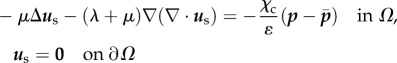
(b) Traction force inverse problem resolution
Details can be found in [27,52,53]. The mechanical characterization of the gel is approximated as isotropic and elastic and the displacements are observed to be small enough so that linear elasticity applies. We assume that the gel can be approximated by a half-space {z ≤ 0}, the gel depth of 70 µm is sufficient to guarantee this for RT112 cells which have a diameter of 50 µm [54], but can introduce an error on some of the frames of the T24 cell migration, since it can transiently reach a length of the order of 100 µm. Following the study of Ambrosi [25], a reduced 2D problem is obtained by averaging in z over an effective thickness w (typically 1.5 µm) and the adjoint problem is written on  in terms of an auxiliary unknown p:
 |
A 1a |
and
 |
A 1b |
where χc is the indicator function of Ωc,  ,
,  is the resultant of p over Ωc and the reduced 2D Lamé coefficients are
  and
and  . Problem (A 1) is solved for all frames i using a finite-element method on a triangulation
  of Ω, where
  are among the nodes and
  is a triangulation of a polygonal approximation Ωc,h of order h2 of Ωc. The calculated traction field is
 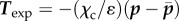 , which vanishes in Ω\Ωc and has zero resultant. For the same reason as the resultant is zero, the torque of the traction field also has to be zero. However, we do not enforce this currently in the method and the fact that the torque is small is only checked a posteriori on the calculated traction field.
(c) Finite-element simulations and parameter fitting
In §3, we derive a tensorial visco-elastic model allowing to predict cell traction field Th from the knowledge of cell shape Ωc and some scalar parameters, namely σa, ζ0, and in the nonlinear case ζ1 and v*. The algorithm for the resolution of the full visco-elastic problem is given in [48]. Here we show in one dimension that within the range of experimentally relevant parameters, visco-elastic effects do not affect strongly the results. Thus simulations are shown only for the reduced viscous limit.
Briefly, we define a finite-element space Vh of piecewise quadratic functions based on the triangulation  of
of  at frame i, where
  is the cell domain Ωc observed experimentally but with distances normalized by D = 50 µm. Using the finite-element software Rheolef, we solve the variational problem, electronic supplementary material, equation (9), in Vh for a given choice of
  and a uniform ζ = ζ0 for a solution
  . In the case of nonlinear friction, ζ depends on v, a fixed-point algorithm is used to construct a sequence of solutions
  using the friction field
 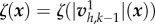 , until convergence.
Next, the parameters can be optimized in order to best fit the experimental observations Texp. Note that best fit is performed on one cell at the initial frame only throughout the paper to acquire parameters σa and ζ0, no fitting is done for the other frames and the other cells. We normalize Texp by a typical value 100 Pa, and aim to minimize  by adjusting ζ0 and σa. Thanks to the linearity of operators and the scale-invariance of our choices for the function ζ (see the electronic supplementary material, text B.2), minimization for a given ζ0 with respect to σa can be done explicitly and the minimization writes:
 |
In the rest of the article, we denote  and
and  simply by Ωc and Texp.
Competing interests
We declare we have no competing interests.
Funding
J.E. thanks the Isaac Newton Institute for Mathematical Sciences for its hospitality during the programme Coupling Geometric PDEs with Physics for Cell Morphology, Motility and Pattern Formation supported by EPSRC Grant Number EP/K032208/1. All authors thank Région Rhône-Alpes (CIBLE), ANR-12-BS09-0020-01 ‘Transmig’ and Tec21 (ANR-11-LABX-0030), and all except A.D. are member of GDR 3570 MécaBio and GDR 3070 CellTiss of CNRS.
References
- 1.Friedl P, Wolf K. 2003. Tumour-cell invasion and migration: diversity and escape mechanisms. Nat. Rev. Cancer 3, 362–374. ( 10.1038/nrc1075) [DOI] [PubMed] [Google Scholar]
- 2.Lauffenburger DA, Horwitz AF. 1996. Cell migration: a physically integrated molecular process. Cell 84, 359–369. ( 10.1016/S0092-8674(00)81280-5) [DOI] [PubMed] [Google Scholar]
- 3.Alt W, Dembo M. 1999. Cytoplasm dynamics and cell motion: two-phase flow models. Math. Biosci. 156, 207–228. ( 10.1016/S0025-5564(98)10067-6) [DOI] [PubMed] [Google Scholar]
- 4.Rubinstein B, Fournier MF, Jacobson K, Verkhovsky AB, Mogilner A. 2009. Actin-myosin viscoelastic flow in the keratocyte lamellipod. Biophys. J. 97, 1853–1863. ( 10.1016/j.bpj.2009.07.020) [DOI] [PMC free article] [PubMed] [Google Scholar]
- 5.Banerjee S, Marchetti MC. 2011. Substrate rigidity deforms and polarizes active gels. Europhys. Lett. 96, 28003 ( 10.1209/0295-5075/96/28003) [DOI] [Google Scholar]
- 6.Lee J, Ishihara A, Theriot JA, Jacobson K. 1993. Principles of locomotion for simple-shaped cells. Nature 362, 167–171. ( 10.1038/362167a0) [DOI] [PubMed] [Google Scholar]
- 7.Pollard TD, Borisy GG. 2003. Cellular motility driven by assembly and disassembly of actin filaments. Cell 112, 453–465. ( 10.1016/S0092-8674(03)00120-X) [DOI] [PubMed] [Google Scholar]
- 8.Bray D, White JG. 1988. Cortical flow in animal cells. Sci. Mag. 239, 883–888. ( 10.1126/science.3277283) [DOI] [PubMed] [Google Scholar]
- 9.Theriot JA, Mitchison TJ. 1992. Comparison of actin and cell surface dynamics in motile fibroblasts. J. Cell Biol. 119, 367–377. ( 10.1083/jcb.119.2.367) [DOI] [PMC free article] [PubMed] [Google Scholar]
- 10.Small JV, Resch GP. 2005. The comings and goings of actin: coupling protrusion and retraction in cell motility. Curr. Opinion Cell Biol. 17, 517–523. ( 10.1016/j.ceb.2005.08.004) [DOI] [PubMed] [Google Scholar]
- 11.Parsons JT, Horwitz AR, Schwartz MA. 2011. Cell adhesion: integrating cytoskeletal dynamics and cellular tension. Nat. Rev. Mol. Cell Biol. 11, 633–643. ( 10.1038/nrm2957) [DOI] [PMC free article] [PubMed] [Google Scholar]
- 12.Stossel TP. 1993. On the crawling of animal cells. Science 260, 1086–1094. ( 10.1126/science.8493552) [DOI] [PubMed] [Google Scholar]
- 13.Verkhovsky AB, Svitkina TM, Borisy GG. 1999. Self-polarization and directional motility of cytoplasm. Curr. Biol. 9, 11–20. ( 10.1016/S0960-9822(99)80042-6) [DOI] [PubMed] [Google Scholar]
- 14.Barnhart EL, Lee KC, Keren K, Mogilner A, Theriot JA. 2011. An adhesion-dependent switch between mechanisms that determine motile cell shape. PLoS Biol. 9, e1001059 ( 10.1371/journal.pbio.1001059) [DOI] [PMC free article] [PubMed] [Google Scholar]
- 15.Blanch-Mercader C, Casademunt J. 2013. Spontaneous motility of actin lamellar fragments. Phys. Rev. Lett. 110, 078102 ( 10.1103/PhysRevLett.110.078102) [DOI] [PubMed] [Google Scholar]
- 16.Barnhart E, Leeb K-C, Allen GM, Theriot JA, Mogilner A. 2015. Balance between cell–substrate adhesion and myosin contraction determines the frequency of motility initiation in fish keratocytes. Proc. Natl Acad. Sci. USA 112, 5045–5050. ( 10.1073/pnas.1417257112) [DOI] [PMC free article] [PubMed] [Google Scholar]
- 17.Recho P, Putelat T, Truskinovsky L. 2015. Mechanics of motility initiation and motility arrest in crawling cells. J. Mech. Phys. Solids 84, 469–505. ( 10.1016/j.jmps.2015.08.006) [DOI] [Google Scholar]
- 18.Alberts B, Johnson A, Lewis J, Raff M, Roberts K, Walter P. 2002. Molecular biology of the cell, 4th edn New York, NY: Garland Science. [Google Scholar]
- 19.Étienne J, Fouchard J, Mitrossilis D, Bufi N, Durand-Smet P, Asnacios A. 2015. Cells as liquid motors: mechanosensitivity emerges from collective dynamics of actomyosin cortex. Proc. Natl Acad. Sci. USA 112, 2740–2745. ( 10.1073/pnas.1417113112) [DOI] [PMC free article] [PubMed] [Google Scholar]
- 20.Oakes PW, Banerjee S, Marchetti MC, Gardel ML. 2014. Geometry regulates traction stresses in adherent cells. Biophys. J. 107, 825–838. ( 10.1016/j.bpj.2014.06.045) [DOI] [PMC free article] [PubMed] [Google Scholar]
- 21.Labouesse C, Verkhovsky AB, Meister J-J, Gabella C, Vianay B. 2015. Cell shape dynamics reveal balance of elasticity and contractility in peripheral arcs. Biophys. J. 108, 2437–2447. ( 10.1016/j.bpj.2015.04.005) [DOI] [PMC free article] [PubMed] [Google Scholar]
- 22.Harris AK, Wild P, Stopak D. 1980. Silicone rubber substrata: a new wrinkle in the study of cell locomotion. Science 208, 177–179. ( 10.1126/science.6987736) [DOI] [PubMed] [Google Scholar]
- 23.Dembo M, Wang Y-L. 1999. Stresses at the cell-to-substrate interface during locomotion of fibroblasts. Biophys. J. 76, 2307–2316. ( 10.1016/S0006-3495(99)77386-8) [DOI] [PMC free article] [PubMed] [Google Scholar]
- 24.Butler JP, Toli-Norrelykke IM, Fabry B, Fredberg JJ. 2002. Traction fields, moments, and strain energy that cells exert on their surroundings. Am. J. Physiol. Cell Physiol. 282, C595–C605. ( 10.1152/ajpcell.00270.2001) [DOI] [PubMed] [Google Scholar]
- 25.Ambrosi D. 2006. Cellular traction as an inverse problem. SIAM J. Appl. Math. 66, 2049–2060. ( 10.1137/060657121) [DOI] [Google Scholar]
- 26.Schwarz US, Gardel ML. 2012. United we stand – integrating the actin cytoskeleton and cell–matrix adhesions in cellular mechanotransduction. J. Cell Sci. 125, 3051 ( 10.1242/jcs.093716) [DOI] [PMC free article] [PubMed] [Google Scholar]
- 27.Peschetola V, Laurent VM, Duperray A, Michel R, Ambrosi D, Preziosi L, Verdier C. 2013. Time-dependent traction force microscopy for cancer cells as a measure of invasiveness. Cytoskeleton 70, 201–214. ( 10.1002/cm.21100) [DOI] [PubMed] [Google Scholar]
- 28.Kruse K, Joanny J-F, Jülicher F, Prost J. 2006. Contractility and retrograde flow in lamellipodium motion. Phys. Biol. 3, 130–137. ( 10.1088/1478-3975/3/2/005) [DOI] [PubMed] [Google Scholar]
- 29.Bangasser BL, Odde DJ. 2013. Master equation-based analysis of a motor-clutch model for cell traction force. Cell. Mol. Bioengng. 6, 449–459. ( 10.1007/s12195-013-0296-5) [DOI] [PMC free article] [PubMed] [Google Scholar]
- 30.Gardel ML, Sabass B, Ji L, Danuser G, Schwarz US, Waterman CM. 2008. Traction stress in focal adhesions correlates biphasically with actin retrograde flow speed. J. Cell Biol. 183, 999 ( 10.1083/jcb.200810060) [DOI] [PMC free article] [PubMed] [Google Scholar]
- 31.Moeendarbary E, Valon L, Fritzsche M, Harris AR, Moulding DA, Thrasher AJ, Stride E, Mahadevan L, Charras GT. 2013. The cytoplasm of living cells behaves as a poroelastic material. Nat. Mater. 12, 253–261. ( 10.1038/nmat3517) [DOI] [PMC free article] [PubMed] [Google Scholar]
- 32.Le Clainche C, Carlier M-F. 2008. Regulation of actin assembly associated with protrusion and adhesion in cell migration. Physiol. Rev. 88, 489–513. ( 10.1152/physrev.00021.2007) [DOI] [PubMed] [Google Scholar]
- 33.Ponti A, Machacek M, Gupton SL, Waterman-Storer CM, Danuser G. 2004. Two distinct actin networks drive the protrusion of migrating cells. Science 305, 1782–1786. ( 10.1126/science.1100533) [DOI] [PubMed] [Google Scholar]
- 34.Yeung T, et al. 2005. Effects of substrate stiffness on cell morphology, cytoskeletal structure, and adhesion. Cell Motil. Cytoskeleton 60, 24–34. ( 10.1002/cm.20041) [DOI] [PubMed] [Google Scholar]
- 35.Burnette DF, et al. 2014. A contractile and counterbalancing adhesion system controls the 3D shape of crawling cells. J. Cell Biol. 205, 83–96. ( 10.1083/jcb.201311104) [DOI] [PMC free article] [PubMed] [Google Scholar]
- 36.Jülicher F, Kruse K, Prost J, Joanny J-F. 2007. Active behavior of the cytoskeleton. Phys. Rep. 449, 3–28. ( 10.1016/j.physrep.2007.02.018) [DOI] [Google Scholar]
- 37.Machado PF, Duque J, Étienne J, Martinez-Arias A, Blanchard GB, Gorfinkiel N. 2015. Emergent material properties of developing epithelial tissues. BMC Biol. 13, 98 ( 10.1186/s12915-015-0200-y) [DOI] [PMC free article] [PubMed] [Google Scholar]
- 38.Étienne J, Duperray A. 2011. Initial dynamics of cell spreading are governed by dissipation in the actin cortex. Biophys. J. 101, 611–622. ( 10.1016/j.bpj.2011.06.030) [DOI] [PMC free article] [PubMed] [Google Scholar]
- 39.He X, Dembo M. 1997. On the mechanics of the first cleavage division of the sea urchin egg. Exp. Cell Res. 233, 252–273. ( 10.1006/excr.1997.3585) [DOI] [PubMed] [Google Scholar]
- 40.Kruse K, Joanny JF, Jülicher F, Prost J, Sekimoto K. 2005. Generic theory of active polar gels: a paradigm for cytoskeletal dynamics. Eur. Phys. J. E 16, 5–16. ( 10.1140/epje/e2005-00002-5) [DOI] [PubMed] [Google Scholar]
- 41.Trichet L, Le Digabel J, Hawkins RJ, Vedula SRK, Gupta M, Ribrault C, Hersen P, Voituriez R, Ladoux B. 2012. Evidence of a large-scale mechanosensing mechanism for cellular adaptation to substrate stiffness. Proc. Natl Acad. Sci. USA 109, 6933–6938. ( 10.1073/pnas.1117810109) [DOI] [PMC free article] [PubMed] [Google Scholar]
- 42.Marcq P, Yoshinaga N, Prost J. 2011. Rigidity sensing explained by active matter theory. Biophys. J. 101, L33–L35. ( 10.1016/j.bpj.2011.08.023) [DOI] [PMC free article] [PubMed] [Google Scholar]
- 43.Recho P, Truskinovsky L. 2013. An asymmetry between pushing and pulling for crawling cells. Phys. Rev. E 87, 022720 ( 10.1103/PhysRevE.87.022720) [DOI] [PubMed] [Google Scholar]
- 44.Ambrosi D, Zanzottera A. 2016. Mechanics and polarity in cell motility. Physica D 330, 58–66. ( 10.1016/j.physd.2016.05.003) [DOI] [Google Scholar]
- 45.Recho P, Truskinovsky L. 2015. Maximum velocity of self-propulsion for an active segment. Math. Mech. Solids 21, 263–278. ( 10.1177/1081286515588675) [DOI] [Google Scholar]
- 46.Recho P, Putelat T, Truskinovsky L. 2013. Contraction-driven cell motility. Phys. Rev. Lett. 111, 108102 ( 10.1103/PhysRevLett.111.108102) [DOI] [PubMed] [Google Scholar]
- 47.Rossier OM, et al. 2010. Force generated by actomyosin contraction builds bridges between adhesive contacts. EMBO J. 29, 1033–1044. ( 10.1038/emboj.2010.2) [DOI] [PMC free article] [PubMed] [Google Scholar]
- 48.Étienne J, Asnacios A, Mitrossilis D, Peschetola V, Verdier C. 2011. How the cell got its shape : a visco-elasto-active model of the cytoskeleton. In Congrès Français de Mécanique, Besançon, France, September 2011. Besançon, France: Presses universitaires de Franche-Comté.
- 49.Étienne J, Hinch EJ, Li J. 2006. A Lagrangian–Eulerian approach for the numerical simulation of free-surface flow of a viscoelastic material. J. Non-Newtonian Fluid Mech. 136, 157–166. ( 10.1016/j.jnnfm.2006.04.003) [DOI] [Google Scholar]
- 50.Rasband WS. 2003–2014 ImageJ. Technical report. Bethesda, MD: U.S. National Institutes of Health. [Google Scholar]
- 51.Ambrosi D, Duperray A, Peschetola V, Verdier C. 2009. Traction patterns of tumor cells. J. Math. Biol. 58, 163–181. ( 10.1007/s00285-008-0167-1) [DOI] [PubMed] [Google Scholar]
- 52.Michel R, Peschetola V, Bedessem B, Étienne J, Ambrosi D, Duperray A, Verdier C. 2012. Inverse problems for the determination of traction forces by cells on a substrate: a comparison of two methods. Comput. Methods Biomech. Biomed. Eng. 15, 27–29. ( 10.1080/10255842.2012.713725) [DOI] [PubMed] [Google Scholar]
- 53.Michel R, Peschetola V, Étienne J, Duperray A, Vitale G, Ambrosi D, Preziosi L, Verdier C. 2013. Mathematical framework for traction force microscopy. ESAIM Proc. 42, 61–83. ( 10.1051/proc/201342005) [DOI] [Google Scholar]
- 54.Lin Y-C, Tambe DT, Young Park C, Wasserman MR, Trepat X, Krishnan R, Lenormand G, Fredberg JJ, Butler JP. 2010. Mechanosensing of substrate thickness. Phys. Rev. E 82, 041918 ( 10.1103/PhysRevE.82.041918) [DOI] [PMC free article] [PubMed] [Google Scholar]
Associated Data
This section collects any data citations, data availability statements, or supplementary materials included in this article.