

Abstract
The interactions of molecules and particles in solution often involve an interplay between isotropic and highly directional interactions that lead to a mutual coupling of phase separation and self-assembly. This situation arises, for example, in proteins interacting through hydrophobic and charged patch regions on their surface and in nanoparticles with grafted polymer chains, such as DNA. As a minimal model of complex fluids exhibiting this interaction coupling, we investigate spherical particles having an isotropic interaction and a constellation of five attractive patches on the particle’s surface. Monte Carlo simulations and mean-field calculations of the phase boundaries of this model depend strongly on the relative strength of the isotropic and patch potentials, where we surprisingly find that analytic mean-field predictions become increasingly accurate as the directional interactions become increasingly predominant. We quantitatively account for this effect by noting that the effective interaction range increases with increasing relative directional to isotropic interaction strength. We also identify thermodynamic transition lines associated with self-assembly, extract the entropy and energy of association, and characterize the resulting cluster properties obtained from simulations using percolation scaling theory and Flory-Stockmayer mean-field theory. We find that the fractal dimension and cluster size distribution are consistent with those of lattice animals, i.e., randomly branched polymers swollen by excluded volume interactions. We also identify a universal functional form for the average molecular weight and a nearly universal functional form for a scaling parameter characterizing the cluster size distribution. Since the formation of branched clusters at equilibrium is a common phenomenon in nature, we detail how our analysis can be used in experimental characterization of such associating fluids.
I. INTRODUCTION
Many complex fluids are composed of highly anisotropic molecules in solution that can be described by a superposition of directional and isotropic intermolecular interactions. To describe these fluids, patch models, which represent molecules as spheres decorated by a constellation of “patches” that introduce directional interactions, provide an attractive minimal model that allows for the study of both liquid-liquid phase coexistence and self-assembly.2 Although such models are applicable to a wide variety of complex fluids, most current work using these models focuses on protein and colloidal solutions.
Patchy models have been used extensively to describe small globular proteins, such as lysozyme and γ-crystallin,3-8 since they gained attention in 1999 due to work done by Benedek and coworkers.9 The introduction of patches represented an advance over prior models that only considered isotropic interactions.10-13 Although the treatment of proteins as spherical particles is simplistic, as detailed by Sarangapani et al.,14 this approach is useful for analyzing scattering data13,15 and for describing the phase coexistence of proteins.3,5,7,8
Recently, Dill et al.8 used a variant of a patch model where the proteins were treated as hard spheres, while the number and interaction strength of the patches were estimated using experimental liquid-liquid phase coexistence curves. In particular, they found that they could reproduce liquid-liquid phase coexistence curves for lysozyme and γ IIIa-crystallin in a phosphate buffer with pH strengths close to seven. However, they did not consider the presence of attractive isotropic interactions (in addition to those of the attractive patches), as Liu et al.5 had done previously. Liu et al. found that spheres with a short-range isotropic interaction and either 4, 5 or 7 attractive patches could also reproduce the liquid-liquid phase coexistence curves of lysozyme and γ-crystallin when normalized by both the critical temperature and density. Dill et al.,8 Liu et al.5 and others3,7 have focused primarily on liquid-liquid phase separation rather than self-assembly, a process that can occur well above the critical temperature for phase coexistence. Experimentally, it is known that proteins form self-assembled clusters, but it is less clear whether the clusters form under equilibrium or non-equilibrium conditions16-22 and how their formation relates to phase coexistence.
Distinct from the case of proteins, patch models have been used extensively to study the self-assembly of synthesized anisotropic particles, in addition to their phase separation.23-29 These studies are fueled by advances in the synthesis of new particles that are anisotropic in shape or interactions, as well as the use of particles in applications including electronics and drug delivery.30-33 For example, one realization of patchy particles uses DNA to provide highly specific interactions,34-37 with recent advances in synthesis allowing for systematic design of patch symmetries and size.36,37 The interactions of such patchy particles can be further controlled by modifying the length, sequence and number of DNA strands.33
Although the patch models are simplistic, they provide a platform for quantifying the role of anisotropic interactions compared to isotropic interactions, an interplay that is clearly of importance in both protein and particle solutions, as well as in molecular fluids with highly directional interactions, e.g., water and alcohols. Using a lattice-based patch model, Frenkel et al.38 identified the critical temperature and critical density for a wide range of both isotropic and patch interaction strengths, as well as various locations and numbers of patches using both simulations and theory. However, they did not compute the liquid-liquid phase coexistence curves nor did they study self-assembly. Roberts and Blanco39 also studied the role of anisotropic interactions, but limited their study to the second osmotic virial coefficient.
The interplay of anisotropic and isotropic interactions has broad significance in the study of the coupling between phase separation and self-assembly. Dudowicz and coworkers40-42 have studied this problem in detail within the context of lattice-based linear polymerization models. They are able to quantify the competition between phase separation and dynamic formation of polymers, a common type of self-assembly process. However, their theory has only been developed for molecules having the equivalent of two spots so that only linear polymers are formed. If more patches are considered, the resulting molecules self-assemble into dynamic, branched polymeric clusters.43-45 This case has received relatively less attention in the literature where the coupling between phase separation and self-assembly are considered.43,46
To quantify the effects of the relative isotropic to anisotropic interaction strength in the context of the practical problem of characterizing protein and patchy particle solutions and to fill a gap in the literature regarding the quantification of coupling between phase separation and self-assembly for multi-functional particles, we study a five spot patch model using both exact Monte Carlo simulations and a renormalized mean-field theory. We expect this generic model of multi-particle association to provide insight into the general pattern of phase separation and self-assembly in complex fluids; thus, we analyze the phase boundaries of these fluids and cluster formation properties including the self-assembly transition lines for cluster formation and percolation, energy and entropy of association, size distributions, and cluster shapes as a function of the relative interaction strength. Although our analysis of the phase boundaries follows the qualitative pattern examined for the two spot case,40-42 the extension to multi-functional association, coupled with both simulations and mean-field theories leads to many new results in comparison to former work.23-26,40-42,46 Specifically, we analytically quantify the relative difference of the simulation and mean-field critical temperatures due to fluctuations absent in mean-field descriptions. Additionally, we identify a universal function for the average cluster size, inspired by mean-field theories, and explore the implications of our results on the interpretation of experimental data.
The paper is organized as follows. In Sec. II, we describe our model of patchy particles, simulation techniques and the renormalized mean-field theory. In Sec. III, we present the liquid-liquid phase coexistence curves, and in Sec. IV, we present thermodynamic transition lines related to the formation of clusters for multiple different relative isotropic to directional interaction strengths. We also analyze the cluster size distribution using geometrical percolation theory and Flory-Stockmayer theory, and we quantify cluster shape and size using the radius of gyration tensor. Finally, we discuss the applicability of our results to experimentally realizable quantities in Sec. V, and in Sec. VI, we summarize the main findings of our work.
II. METHODS
A. Patchy Particle Model
Our patchy particles consist of spheres with diameter σ that are decorated with five completely penetrable, smaller spheres, or patches, of diameter δσ. The smaller spheres are arranged in a dipyramid shape with the center of the smaller spheres located at the edge of the larger sphere (see Fig. 1). The large spheres interact with an isotropic square well potential:
| (1) |
where ri is the distant between the centers of the large spheres. The small spheres located on different particles interact through a purely attractive square well potential:
| (2) |
where rp is the distance between the centers of the small spheres. We chose , which is the largest size where geometric constraints dictate that patchy “bonds” only occur between two, rather than three or more particles; this choice allows for comparison with theory. We choose the isotropic range λ = 1.15 consistent with the model of Liu et al.5 Since the interactions are attractive and short-ranged, the isotropic term can be thought of qualitatively as a van der Waals interaction.
FIG. 1.
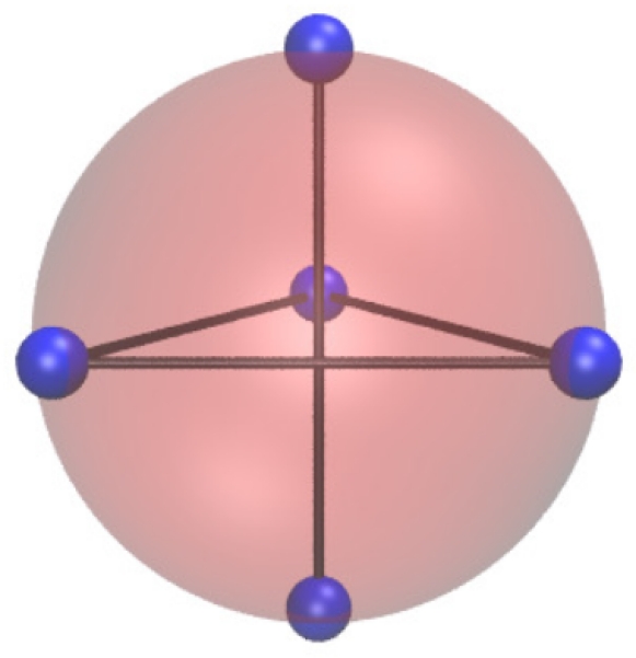
Monomer with location of five spots shown. Lines emphasize the geometry. This image was made with VMD software support.47
B. Monte Carlo Simulations
For the calculation of the liquid-liquid phase coexistence, we applied the transition matrix Monte Carlo (TMMC) method, as described in Ref. 48. TMMC was performed in the grand canonical ensemble where the number of particles N varies during the course of the simulation. For efficiency, each individual simulation considers only a range of N, specifically, from Nmin to Nmax. Due to the computational expense of simulations sampling large N, the range of particles is chosen to decrease with increasing Nmin. In particular, Nmin = N0n2/3 where N0 is a prefactor, n is the simulation number, and Nmax is chosen such that there is an overlap of four values of N, i.e. Nmax = N0(n + 1)2/3 + 4. For example, taking N0 = 164, simulation numbers 0, 1 and 2 have [Nmin, Nmax] ranges of [0, 168], [164, 264] and [260, 345], respectively. Each simulation was run across 12 cores with the particle range determined using a similar method. Specifically, for odd processor number p, the range is [Nmin + c(p − 1)2/3, Nmin + c(p + 1)2/3 − 1], and for even processor number p, the range is [Nmin+(c/2)((p−2)2/3+p2/3), Nmin+(c/2)(p2/3+(p+2)2/3)−1] where c = 0.202(Nmax−Nmin). Such a choice allows for a large overlap in order to facilitate equilibration through swaps in particle range between processors.
All simulations were initialized without any particles in order to ensure random initial configurations and were only limited to their specified ranges once Nmin was achieved. At each Monte Carlo step, one of four types of moves were attempted: single particle insertions (10 % probability), single particle deletions (10 % probability), single particle rotations (40 % probability) or single particle displacements (40 % probability). Every 108 Monte Carlo moves, simulations on different cores were allowed to swap their Nmin and Nmax if their N ranges overlapped. The target maximum displacement and maximum rotation angle were updated with a target acceptance rate of 50 %. Finally, the probability distributions of sampling N particles were updated using data across all 12 cores. Simulations continued until each N was visited 25,000 or more times from a different N. Normally, each N was visited from a different N close to 107 times for N less than 150 and close to 106 for almost all N up to 900, with the exception of the patchy limit ϵi = 0. The probability distributions from each simulation were then stitched together by matching the probability distributions at the largest N for the simulation with fewer particles, and demanding normalization. Finally, reweighting of the chemical potential was used to find the condition where the areas under both the low density and high density curves were equal, which was then used to define the average density in both the dilute and rich phases.
The corresponding critical point for the liquid-liquid phase separation was estimated using fits to the structure factor in the one phase region. Details of this technique can be found in the Supplementary Information (SI). Our results agree with standard scaling expressions for critical properties of theories that incorporate fluctuation effects by altering the critical exponents from their mean field theory values.49
For the one phase region, canonical Monte Carlo simulations were run with a 50 % probability of single particle displacement and a 50 % probability of single particle rotation at each Monte Carlo step. For densities ρ ≡ N/V < 0.8 σ−3, the initial configuration was generated via a grand canonical simulation until the desired density was reached. For ρ ≥ 0.8 σ−3, this procedure was prohibitively computationally expensive to perform for each simulation, so it was performed once to generate a random initial condition that was then used for all temperatures and interaction strengths considered. The maximum displacement distance and maximum rotation angle were chosen such that moves were accepted roughly 50 % of the time. After the maximum displacement and maximum angles were determined, the simulations were run for 5 × 10⁹ Monte Carlo steps; the first 5 × 10⁸ Monte Carlo steps were discarded in order to ensure the equilibration of the system. For calculations of the heat capacity, simulations were run for 5 × 10¹⁰ Monte Carlo steps, and the first 5 × 10⁹ Monte Carlo steps were discarded in analysis. The heat capacity was computed for each temperature and density using fluctuations of the potential energy (e.g., (〈U2〉 − 〈U〉2)/(kBT2)); uncertainty was determined using a standard error analysis.50 The maximum heat capacity was estimated by fitting a quadratic function to the heat capacity data in the vicinity of the maximum.
All simulations were run using a cubic box size of edge length 10 σ with periodic boundary conditions such that the volume V = 1000 σ3. The metrics for clustering only weakly depend on box size at this size (see comparison to a smaller box size in the SI). For consistency, the same box size was used for the phase separation.
C. Renormalized Mean-Field Theory
To describe our system using theory, we use a statistical associating fluid theory for variable range potentials (SAFT-VR)51 and subsequently apply a renormalization technique. In SAFT-VR, an approximate theory, the Helmholtz free energy normalized by the number of particles is given by
| (3) |
where the subscripts id, i and p correspond to the ideal, isotropic square well and patchy contributions, respectively. The ideal part of the free energy is given by
| (4) |
where β ≡ 1/(kBT), kB is Boltzmann’s constant, T is temperature, ρ is the number density, and λT is de Broglie’s wavelength.
The isotropic contribution to the free energy, treated using an inverse temperature expansion,52,53 is described by a sum of three contributions
| (5) |
where βfhs is the hard sphere contribution and βfsw,1 and β2fsw,2 are the first and second perturbation terms. From Carnahan and Starling54, the hard sphere contribution is approximated as
| (6) |
where the packing fraction ϕ = ρσ3π/6. Following Gil-Villegas et al.,51 the two square well contributions are
| (7) |
and
| (8) |
where the effective volume fraction is ϕeff = 0.859413ϕ − 0.153391ϕ2 − 0.121318ϕ3 for the isotropic range λ = 1.15.
The patch contribution to the free energy, estimated using Wertheim’s thermodynamic perturbation theory,55-57 is
| (9) |
where Mp is the number of patches and X is the fraction of patches that are non-bonded,
| (10) |
The patch interaction strength is
| (11) |
Here, r12 is the distance between two particles, gsw is the reference pair correlation function, f(12) = e−βup − 1 is the Mayer f function,58 and 〈f(12)〉ω1,ω2 is the Mayer f function averaged over all orientations,
| (12) |
with S(r) = (δσ+σ−r)2(2δσ−σ+r)/(6σ2r).25 Note that the Mayer f function only includes the patch interactions, since the isotropic interactions are contained in the reference pair correlation function, gsw(r12), which is approximated by its value at contact, since the range of interaction is short. In turn, the contact value, gsw(σ), is approximated as51
| (13) |
Here, the first term represents the hard sphere radial distribution function and the following two terms together yield the term in the free energy expansion. Note that only a n − 1 order expansion is required for structural quantities such as g(r) in order to be consistent with n order expansion for thermodynamic quantities such as f.51 Using the above approximations, the patchy interaction strength simplifies to the form
| (14) |
where the bonding volume Vb = πδ4 σ3(4δ + 15)/30.
However, it is evident that this theory involves a number of approximations and thus fails to recover the correct “theta” temperature Tϴ, or “Boyle temperature,” defined as the temperature at which the second osmotic virial coefficient B2 vanishes, i.e., B2(Tϴ) = 0. This defect in the analytic theory can be corrected by redefining the isotropic interaction strength so that the theory exactly recovers Tϴ, a basic measure of interparticle interaction. We refer to the resulting analytic model as the renormalized mean-field theory (RMFT). Such a renormalization also yields an improved estimate of B2 across the full range of temperatures (see SI) and should minimize errors due the inverse temperature expansion meaning that the main effect of deviations between RMFT and simulation will be due to the mean-field approximation rather than other approximations. The need for a theory whose deviations are primarily due to only the mean-field approximation will be apparent in Sec. III.
The first step in the renormalization procedure involves determining B2 for the exact model and the approximate theory. In particular, B2 can be exactly computed for our model using the Mayer cluster formalism59
| (15) |
where r12 is the distance between the center of mass of the two particles, Ωj is the orientation of particle j, u is the total potential energy including both isotropic and patch contributions. Evaluating the above quantity yields
| (16) |
with representing the hard sphere virial. For the approximate liquid state theory described above, B2 can be computed by expanding the compressiblity factor in density and taking the coefficient of the first order term. Such a calculation results in the relation
| (17) |
The second step in the renormalization procedure involves determining the renormalized ϵi, for ϵi ≠ 0. For clarity, we switch to energy and temperature scales relative to the patch energy ϵp. Next, we compute the exact, analytic value of Tϴ for a given ϵi. We then determine a renormalized value of , by requiring exactly. Then is used in place of ϵi within the theory to yield the renormalized mean-field theory (RMFT). This procedure ensures that the mean-field theory produces the correct theta temperature for our molecular model. The dependence of on ϵi is shown in the SI.
Using the above theory, the critical point is determined by simultaneously requiring ∂3(ρf)/∂ρ3 = 0 and ∂2(ρf)/∂ρ2 = 0. The phase coexistence is determined by minimizing the total free energy density of the system, i.e., ρT fT = (ρT − ρ2)/(ρ1 − ρ2)ρ1f(ρ1) + (ρT − ρ1)(ρ2 − ρ1)ρ2f(ρ2) with respect to ρ1 and ρ2 subject to 0 ≤ ρ1 ≤ ρT and ρT ≤ ρ2 ≤ 6/(πσ3). ρT is the initial concentration and always chosen to be the critical density. This procedure is a Gibbs ensemble formulation60 and is equivalent to requiring that the chemical potentials and pressures are equal in both phases.
For conciseness, we define energy and temperature scales relative to the patch energy strength ϵp, and lengths relative to the hard sphere diameter σ for the remainder of the paper.
III. PHASE SEPARATION
Prior to investigating self-assembly, we determine the location of the liquid-liquid phase coexistence curves as a function of the isotropic interaction strength ϵi, where ϵi is in reduced units and thus represents the relative isotropic to directional interaction strength. In Fig. 2, we show the phase boundaries obtained by Monte Carlo simulation and renormalized mean-field theory (RMFT). In both cases, the critical density ρc and temperature Tc shift to smaller values with decreasing ϵi, although the shift is more pronounced for the analytic theory. A prior study24 on the numbers of patches in the ϵi = 0 limit found that the critical density decreases with decreasing number of patches and becomes zero in the two spot case.24 In this sense, making the number of patches large qualitatively corresponds to an isotropic potential, so the trend for ρc and Tc with increasing ϵi is consistent with the earlier work. Additionally, the non-zero critical density for patch numbers greater than two is fundamentally different than the two spot case where only linear chains can form. Previous work has attributed shift to a constant non-zero ρc in the ϵi = 0 limit to the presence of cooperative interactions due to competitive equilibria.61
FIG. 2.
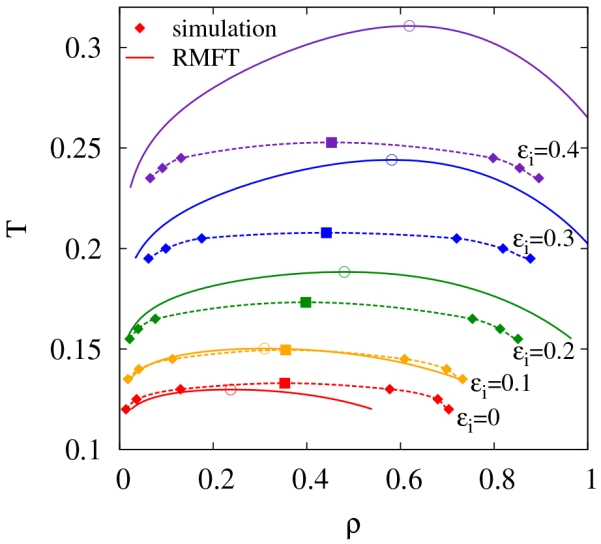
Phase coexistence curves for both simulation and renormalized mean-field theory (RMFT) for different interaction strengths (ϵi). Simulation critical points are estimated from analysis of scattering data coupled with rectilinear diameters. Dashed lines are only for guidance.
It is apparent from Fig. 2 that the RMFT becomes an increasingly accurate description of the simulation data for small values of ϵi. In order to explore this further, we plot the critical temperatures for both simulation Tc,sim and RMFT Tc,RMFT along with the theta temperature Tϴ in Fig. 3a. As mentioned in Sec II, the Tϴ corresponds to the temperature at which the second osmotic virial coefficient B2 = 0. Examples of B2 as a function of temperature for different values of ϵi can be found in Fig. 3b. Due to the renormalization technique employed in the RMFT, the Tϴ for both the simulation and RMFT is equal, by definition (see Eq. 16). Due to critical fluctuation effects, which are absent in RMFT (as well as all analytic theories of phase separation in three dimensions), we would expect deviations between Tc,RMFT and Tc,sim. However, these deviations, surprisingly, almost vanish as the purely patchy limit is approached (i.e., small ϵi). This striking effect, that fluctuation effects are weak in the patchy limit, is apparent in former simulations but has not been explained previously.24,62 In the patchy limit, ϵi = 0, the ratio of Tϴ to Tc approaches a constant that is greater than 1, the limit for long permanent homopolymers.
FIG. 3.

(a) Theta temperature for the model along with critical temperatures for both simulation Tc,sim and renormalized mean-field theory (RMFT) Tc,RMFT. (b) The second osmotic viral coefficient B2 for various interaction strengths (ϵi). (c) Ratio of Tc,sim to Tc,RMFT from simulations. The dotted line corresponds to an estimation of the critical fluctuation effects as described in the text.
In order to quantify the critical fluctuation effects as a function of ϵi, we plot the ratio of Tc,sim to Tc,RMFT (Fig. 3c). In the limit that ϵi → ∞, we expect this ratio to be less than 1 and comparable to the corresponding estimate for the Ising model in three dimensions with a nearest neighbor interactions, Tc,sim/Tc,RMFT = 0.752.63,64 This ratio is nearly independent of lattice64 suggesting its applicability off-lattice fluids. Further, an expansion of Tc,sim/Tc,RMFT in terms of the lattice coordination number q yields,65-67
| (18) |
We can translate Eq. 18 into a corresponding result for an off-lattice fluid by calculating the B2 of a lattice fluid, as well as that of a square well fluid in the continuum. Direct correspondence implies that q in the lattice model corresponds to the dimensionless interaction range variable λ of the square well potential, i.e., q ∝ λ3 − 1.67-69 Thus, we have
| (19) |
where we take a0 to be a constant that exactly recovers the nearest-neighbor Ising result in the limit ϵi → ∞. For λ = 1.15, this condition implies a0 = 0.129 by consistency. Since λ3 − 1 can be taken as the prefactor to (eβϵi − 1) in B2 (Eq. 16), B2 can also be used to determine an effective range parameter ; for any ϵi by following the same principle,
| (20) |
We also need the temperature, which we chose to be Tc,RMFT, in order to fully specify . Combining this information with the value of a0 from our continuum potential model and Eq. 19 with the replacement of λ by allows for a prediction of Tc,sim/Tc,RMFT, using only system parameters and RMFT. Fig. 3c shows the resulting prediction as a dotted line. There seems to be a constant shift of ≈ 0.03 between our theoretical estimates and measured ratios, but this discrepancy is likely due to the inherent approximations of the RMFT. Given these approximations, we view the similarity of the results as quite encouraging. Additionally, the analysis indicates that RMFT works better at smaller values of ϵi because the effective coordination number of the intermolecular interaction increases as ϵi decreases, an effect that is naturally associated with large clustering near the critical point. We emphasize that this prediction requires no knowledge from simulation. Thus, it can be used to estimate the phase boundaries with fluctuations based on only RMFT. Of course, separate arguments will have to be considered to estimate the correct critical density with fluctuation effects included.
IV. SELF-ASSEMBLY
A. Self-assembly transition lines
In addition to phase separation, due to their patchy nature, our particles form dynamic clusters upon cooling, where clusters are uniquely defined through associative patchy interactions. In our case, clusters can be defined without the introduction of a cut-off distance, since the patchy potential is prescribed by a square well interaction. Fig. 4 illustrates examples of different clusters obtained from simulation. It is clear that the clusters resemble highly branched polymers. They also contain multiple branch points and loops, and form and disintegrate in dynamic equilibrium. Prior to quantifying the cluster distributions and sizes of these clusters, we first consider two metrics that can be used to define polymerization transition lines governing the self-assembly, as opposed to the liquid-liquid phase separation boundaries. As this process of self-assembly does not involve discontinuities in any of the derivatives of the free energy, these polymerization transition lines highlight the progress of self-assembly, rather than a phase transition proper. Nonetheless, it has been shown that the polymerization transition lines for linear polymers can be described as a line of “rounded,” thermodynamic transitions70,71 that can be mathematically described by an interacting spin model with an applied magnetic field controlling the degree of “rounding” or “cooperativity”.72 We expect that a similar situation is true for our branched polymeric clusters.
FIG. 4.
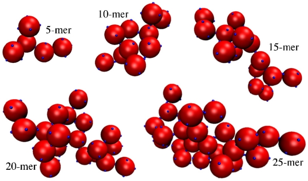
Example clusters of various sizes. This image was made with VMD software support.47
The first metric for describing the emergence of self-assembly is the extent of particle cluster formation Φ, also referred to as the extent of polymerization. Φ is defined as the average fraction of particles that are in clusters, as opposed to being in a monomeric state, which is given by 1 − Φ. This quantity represents an order parameter for the self-assembly.40-42 Simulation results for Φ are plotted as points in Fig. 5a for ϵi = 0.1, various temperatures and various densities. When either the temperature is lowered or the density is increased, Φ, and thus the number of particles in clusters, increases. Since the predictions for Φ as a function of T from RMFT do not exactly overlap with the simulation data, we use the functional form from RMFT to obtain accurate estimates for Φ at intermediate temperatures. Specifically,
| (21) |
where X is the probability that a patch is not bonded and is given analytically by Eq. 10; thus 1 − X5 is the probability that there is at least one bonded patch. The exponent 5 signifies the number of patches per particle. Combining the relation between Φ and X (Eq. 21), the relation between X and Δ (Eq. 10), and the expression for Δ (Eq. 14) yields the functional form for RMFT,
| (22) |
with the parameters aΦ and bΦ defined exactly within RMFT given both ϵi and ρ. Since the theory does not match the simulations exactly, we let aΦ and bΦ become fitting parameters. Note that bΦ is exactly 0 for the case of ϵi = 0, and thus it is not used as a fitting parameter in this limit. As can be seen from Fig. 5a, this procedure provides an excellent fit to the simulation data.
FIG. 5.

(a) The order parameter Φ and (b) the probability of percolation pperc as a function of temperature for densities ranging from 0.1 to 0.9. The interaction strength ϵi is 0.1. Points are simulation data, and lines are fits that are detailed in the text.
In order to characterize the assembly process, we also identify the thermodynamic conditions at which percolating, or system spanning clusters become significant in our simulations. Following standard arguments of simple geometrical percolation theory,73 we consider the probability that one or more clusters of associated particles percolate across the simulation box at any given time during the course of the simulation as our second metric for self-assembly. Note that unlike simple geometrical percolation theory, clusters are defined through patch interactions rather than proximity. The resulting percolation probability is plotted as points in Fig. 5b for ϵi = 0.1. The data at low temperatures is cut-off due to intersection with the phase coexistence curves. The lines are fits assuming that the distribution follows 1/2(1 − erf[(T − ΔT)/w] where ΔT and w are fitting parameters that are dependent on the density.73 As simulation box size increases, these curves in Fig. 5b should approach Heaviside step functions in the thermodynamic limit; however, finite size effects cause a rounding of this transition.73 Fortunately, the temperature at which the probability of percolation, pperc, equals 1/2 denoted by Tpperc=1/2 is only slightly sensitive to the simulation box size (see SI for details), and thus, Tpperc=1/2 can be used with minimal concern regarding finite size effects. Interestingly, when pperc = 1/2, Φ varies only slightly, ranging from 0.83 to 0.89 suggesting that knowledge of Φ alone may serve as a rough criterion for describing the state of self-assembly. This point will be explored extensively below.
These metrics are then used to define polymerization transition lines, which in turn define the continuous process of particles associating into polymeric structures. For a given density and ϵi, the temperatures at which Φ = 1/2, ∂2Φ/∂T2 = 0 (inflection point) and pperc = 1/2 define polymerization transition lines. These transition lines are denoted as TΦ=1/2, TΦ, infl and Tpperc=1/2, respectively. Fits to the simulation data, such as that in Fig. 5a, is used to identify the transition lines based on Φ, while linear interpolation is used for the transition lines based on pperc. These transition lines are represented by points in Fig. 6 for various values of ϵi. For comparison, estimates of the phase boundaries from simulation (see Fig. 2) are shown as dashed lines. Theoretical Φ based transition lines are computed with RMFT, since Φ = 1 − X5 with X given by Eq. 10. Interestingly, there is a cross over point in these transition lines for different values of ϵi at densities around 0.75. In RMFT, Φ is calculated directly from X, and the only dependence on ϵi occurs in the reference radial distribution function. At the observed crossover point in RMFT where Φ does not depend on ϵi, the square well contributions to the reference radial distribution function perfectly cancel such the the radial distribution function is equal to the hard sphere radial distribution function (see Eq. 13 noting that the first term is the hard sphere contribution).
FIG. 6.
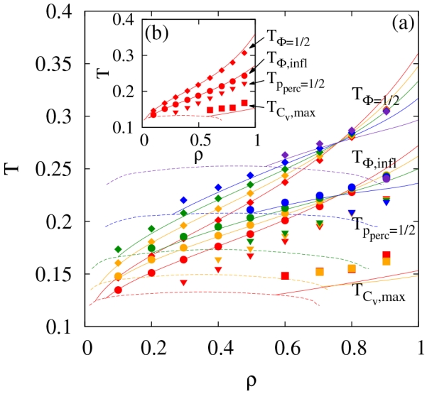
(a) Metrics for clustering transitions for both simulation (points) and renormalized mean-field theory (solid lines). Dashed lines represent rough estimates of phase boundaries. Interaction strengths considered are ϵi = 0, 0.1, 0.2, 0.3 and 0.4 with the lowest data representing ϵi = 0. (b) Values for only ϵi = 0 for clarity.
The maximum in the heat capacity is also used as a metric for self-assembly and is directly determinable via experiments. Thus, this metric is shown in Fig. 6 for both simulations and RMFT. For the simulations, it is difficult to determine precise values of the maximum heat capacity, and based on our fits, we estimate the uncertainty to be roughly twice the symbol size. Note that the RMFT for the maximum heat capacity deviates from the simulation data much more than in the case of Φ based transition lines for reasons that are not clear.
Together, the four polymerization transition lines displayed in Fig. 6 provide a characterization of the self-assembly present in our system. Specifically, at very high temperatures all of the particles are in a monomeric state. Then, as the temperature lowers, they start to form dynamic, branched, polymeric clusters with exactly half of the particles in clusters on average at TΦ=1/2. As the temperature continues to lower, the clustering speeds up until TΦ,infl is reached. Eventually, system spanning clusters form at Tpperc=1/2, which occurs at even lower temperatures. Finally, a maximum in the heat capacity is observed at significantly lower temperatures assuming that phase separation did not occur first. Compared to the two spot model, the difference between TΦ=1/2 and TΦ,infl is much greater,25 which could be predicted a priori given the RMFT.
Perhaps the largest effect of ϵi is in the relative locations of the polymerization transition lines compared to the phase separation curves. When the patch strength is much stronger than the isotropic strength, the region in which clustering occurs is significantly larger and extends to lower densities. This trend holds regardless of the temperature reference used (see SI for details).
B. Entropy and energy
In addition to determining the location of relevant transition lines, we determine entropy and energy of association using the RMFT and values for Φ, and thus X, from simulation. Specifically, a rearrangement of Eq. 10 yields a chemical equilibrium form of the formation of bonds between two particles, which can then be used to identify an equilibrium constant Kb as in Ref 25.
| (23) |
In turn, Kb can be used to extract both the energy ΔU and entropy ΔS via the Helmholtz free energy ΔF for the formation of the bonds between two particles,
| (24) |
Using the same functional form as the RMFT (see Eq. 22), the functional form of the equilibrium constant is
| (25) |
Here aΦ and bΦ are parameters that are uniquely determined within the RMFT by ρ and ϵi. Assuming that e1/T >> 1, which should hold for temperatures that are low enough to observe self-assembly, this term can be approximated by e1/T allowing for the determination of both the energy and the entropy via thermodynamic definitions. The limit where aΦ >> bΦϵi/T permits the further approximations:
| (26) |
| (27) |
Although this further approximation is not yet justified, its value will become apparent. By combining Eqs. 23, 24, 26, and 27, we find
| (28) |
The above expression can be simplified by recasting ln aΦ + ln ρ in terms of TΦ=1/2 (by plugging both T = TΦ=1/2 and X = 1 − Φ1/5 = 1 − (1/2)1/5 into Eq. 28 and solving for ln aΦ + ln ρ). Plugging this result back into Eq. 28 yields the simple form:
| (29) |
This functional form allows for the identification of both the energy and the entropy through the use of an Arrhenius plot (see Fig. 7). In particular, the entropy of association becomes
| (30) |
where TΦ=1/2 is density dependent and the ln (21/5(21/5 − 1)) term must be modified for a different choice of Mp. The points are simulation results determined using MpρΔ = (1 − X)/X2 and the line is generated using Eq. 29. Due to the quality of the fit, we can confirm the consistency of the approximations and that a general graph of MpρΔ versus 1/T can be used to extract both the energy through the negative of the slope of such a graph and the entropy. The implications of this scaling for the interpretation of experimental data is discussed in Sec. V.
FIG. 7.
An Arrhenius plot to illustrate the ability to extract the energy and entropy of self-assembly. Points are simulation data, and the line is derived in the text.
C. Quantifying cluster size and shape
Having identified the entropy and energy of association and thermally reversible polymerization transition lines, in addition to the phase boundaries, we now focus on the cluster distributions, as well as the cluster sizes and shapes under different thermodynamic conditions from our simulations. In Fig. 8, we show the distribution p(M) of clusters of size M for a wide range of temperatures, densities, and ϵi for state points above the percolation transition line. In order to characterize these distributions, we make use of two different theories. The first is a scaling framework that assumes the applicability of geometrical percolation theory to our dynamically associating particles;73 the second is Flory-Stockmayer74,75 mean-field theory.
FIG. 8.
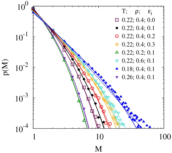
Cluster size distributions for various parameters from simulations (points). Dashed lines are predictions from Flory-Stockmayer theory given the value of the order parameter and solid lines are fits from geometrical percolation theory.
For non-percolating systems, the probability distribution for observing clusters of size M within geometrical percolation theory is given by
| (31) |
where μ represents a metric of size, and τ represents the power law associated with the distribution. In Eq. 31, Li is the polylogarithm function and results from normalization so that the sum of p(M) over all values of M equals 1. Treating τ and μ as free parameters, the fits using geometrical percolation theory are shown as solid lines in Fig. 8. Within geometrical percolation theory, the probability distribution function formally applies up to the percolation transition, at which point μ diverges and the probability distribution becomes a power law. However, this approach requires two fitting parameters and the variation of the fitting parameters is not known a priori, since geometrical percolation theory is based on a different type of percolation than observed in our system. Thus, we also consider the applicability of the mean-field theory of Flory and Stockmayer.74,75
Within Flory-Stockmayer theory, the probability distribution for observing clusters of size M is given by
| (32) |
This equation assumes that no loops are formed, an assumption that clearly becomes invalid at even moderate cluster sizes (loops can be clearly seen in Fig. 4) and that the percolation has not yet been reached. The later assumption is quantified within the theory by requiring X be larger than its value at percolation, 3/4. Since X is directly related to Φ (see Eq. 21), the Flory-Stockmayer cluster distributions can be generated from knowledge of Φ from the simulations and thus requires no fitting parameters. These predictions are shown in Fig. 8 as dashed lines. Despite the fact that the assumptions for Flory-Stockmayer do not apply for small M, the predictions are in good agreement with the simulations, suggesting that Flory-Stockmayer theory may be used to gain further insight into the system regardless of its approximate nature. The highly attractive feature of Flory-Stockmayer theory is that it can roughly reproduce the correct distribution with minimal information. Specifically, since there is only one parameter, this parameter can be determined through knowledge of only the average cluster size 〈M〉 (see Eq. 33) meaning that a good estimate of p(M) can be determined from a single experimental measurement.
We also explore the shape of the branched, polymeric clusters from our simulations. We do not include system spanning clusters, since they are, for a periodic system, infinite clusters. As can be seen in Fig. 9, the radius of gyration Rg scales as M to a power near ν ≈ 1/2 for a wide range of conditions, including different temperatures, densities and ϵi. This means that the fractal dimension of the non-percolating clusters df = 1/ν ≈ 2, which is the known value for lattice animals,76 but distinct from geometrical percolation clusters where the fractal dimension is near 2.5.73 Lattice animals are in the same universality class as branched polymers swollen by excluded volume interactions, while geometrical percolation clusters are in the same universality class as branched polymers with screened excluded volume interactions or at their theta point.77 This suggests that our clusters are in the swollen, branched polymer universality class. For comparison, the mass scaling exponent for the mean-field Flory-Stockmayer theory is 1/4, reflecting the mean-field nature of this model and the large upper critical dimension of 8, above which excluded volume interactions can be neglected.73 Evidently, configurational fluctuations lead to large deviations from mean-field predictions regarding polymer size.
FIG. 9.
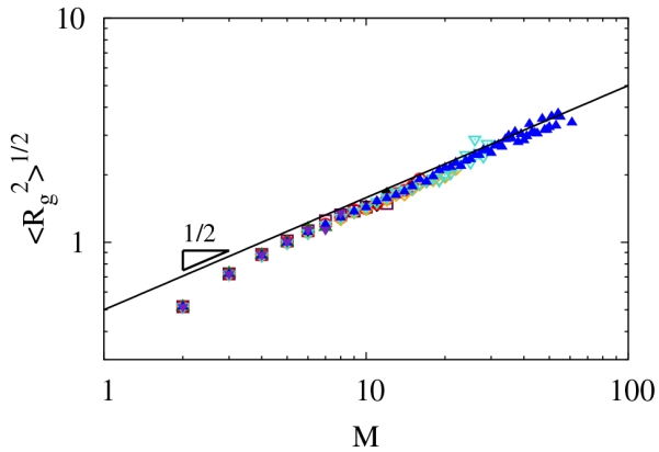
Radius of gyration for various parameters (symbols are the same as Fig. 8). System spanning clusters were not considered and at least five samples were required for averages.
To further quantify the shapes of the clusters, we compute the ratios of the average values of the eigenvalues of the radius of gyration tensor for the same clusters, shown in Fig. 9. We label the eigenvalues, λi such that λ1 ≤ λ2 ≤ λ3. Note that by definition or, equivalently, . The ratios are plotted in Fig. 10. For perfectly isotropic clusters both ratios, λ3/λ1 = λ2/λ1 = 1. Small clusters are highly anisotropic, but this is not surprising given that two of the eigenvalues are zero for a dimer. As the cluster size increases, the ratios asymptote to a result near the expected value for lattice animals, rather than geometrical percolation clusters.78 This finding is consistent with our analysis of the fractal dimension. However, for clusters with very large masses, it is reasonable to expect that the excluded volume interactions would be screened, implying that the scaling exponent should approach that of geometrical percolation clusters due to screening of excluded volume interactions. Finite size limitations do not permit a definite conclusion regarding such a trend.
FIG. 10.
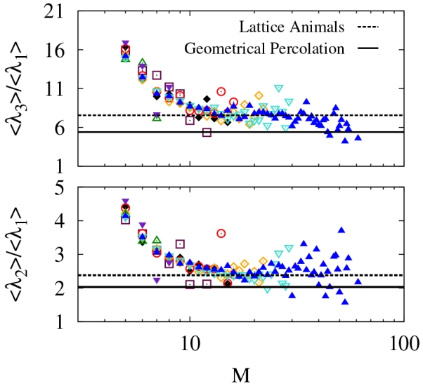
Ratios of average eigenvalues of the radius of gyration tensor for various parameters (symbols are the same as Fig. 8). The eigenvalues are sorted by magnitude such that λ1 ≤ λ2 ≤ λ3. System spanning clusters were not considered and at least five samples were required for averages.
D. Universal descriptors of cluster size
Having quantified cluster size distributions, as well as the cluster sizes and shapes from simulation, we investigate the average cluster size 〈M〉, which we plot as a function of density for various temperatures in Fig. 11a. We observe larger average cluster sizes both at lower temperatures and higher densities. Such trends follow intuition and qualitatively accord with experimental results for the average size of lysozyme clusters.21 If we plot 〈M〉 as a function of the order parameter Φ instead of density, 〈M〉 for all densities, temperatures and ϵi above the percolation transition line roughly follow a master curve as can be seen in Fig. 11b. Using Flory-Stockmayer theory, this relationship equals79
| (33) |
where X is determined by Φ = 1 − X5. This relation is expected to hold for X > 3/4 or equivalently, Φ ≤ 0.763. As can be seen from Fig. 11b, Flory-Stockmayer theory agrees nearly perfectly with our simulation results within the range in which it is applicable. A linear plot can also be generated by plotting 1/〈M〉 versus X as shown in the SI. For larger values of Φ, the relation breaks down, due to both the formation of percolating clusters and the presence of loops.
FIG. 11.
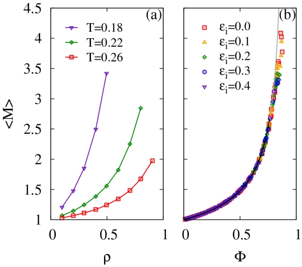
(a) The average cluster size for various temperatures as a function of density from simulations. The interaction strength was chosen to be ϵi = 0.1. (b) Average cluster size as a function of the order parameter from simulations. The line is the prediction from Flory-Stockmayer theory, does not include any fitting parameters. The extension of the line beyond its validity of Φ ≤ 0.763 is in gray.
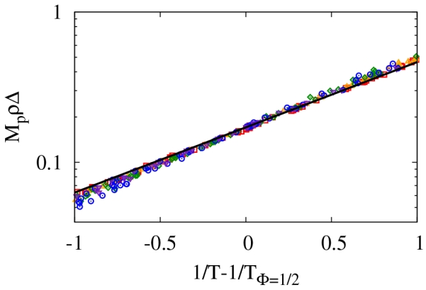
We now explore if we can obtain a universal description of the T dependence of 〈M〉. Inspired by the Arrhenius description, which clearly links 〈M〉, and thus X, to T, we plot 〈M〉 as a function of 1/T − 1/TΦ=1/2 in Fig. 12 yielding a master curve. This master curve follows the expected function, shown as a black line. The function is determined by solving Eq. 29 for X and then plugging the result in Eq. 33. Small deviations at larger values of 1/T are due to the breakdown of the Flory-Stockmayer relation (Eq. 33).
FIG. 12.
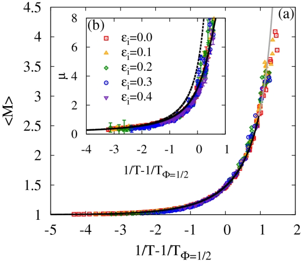
(a) Average cluster size and (b) the fitting parameter μ in geometrical percolation theory as a function of inverse temperature minus the inverse of the Φ = 1/2 polymerization transition temperature for all densities, temperatures and ϵi above the percolation transition. Points correspond to simulation data. The solid lines describe the shape of the master and master-like curves, while the dashed line represents the Flory-Stockmayer prediction of μ without any fitting parameters (see text for details). The line in gray denotes an extension of the curve beyond its range of validity.
Similar to the universal 1/T − 1/TΦ=1/2 dependence of 〈M〉, we consider if the characteristic cluster size parameter μ from percolation theory (see Eq. 31) also has a master curve (the inset to Fig. 12). Here the data reduction is not a true master curve, as there are small but systematic deviations for different interaction strengths. To provide an approximate analytic form for the T dependence of μ and 〈M〉 that would be valuable for describing experimental data, we again turn to the Flory-Stockmayer theory, since, despite its deficiencies, it is able to provide physical insight into the cluster size distribution and cluster size average. Specifically, in the large M limit Flory-Stockmayer theory reduces to the closed form:
| (34) |
Comparing the above equation with the probability distribution expected from geometrical percolation theory (see Eq. 31), one finds the Flory-Stockmayer result corresponds to τ = 5/2 and
| (35) |
Although Flory-Stockmayer predicts τ = 5/2, our fits indicate that it ranges from roughly 1.7 to 2 for T > TΦ=1/2, which is consistent with the expected range for lattice animals,78,80 but different from τ = 2.18, the expected value from geometric percolation theory estimate for randomly placed non-interacting particles.73 Thus, in our quantification of the relationship between μ and temperature, we consider only the functional form for μ suggested by Flory-Stockmayer theory. Accordingly, we let ln(27/256) become a fitting parameter y and find that a fit of − ln(X3(1 − X)) versus 1/μ yields y = −2.146 ± 0.003, as compared to the Flory-Stockmayer prediction of −2.249. The results of this fit, which relate μ to X can then be combined with the relationship between X and 1/T − 1/TΦ=1/2 to yield the black line in the inset of Fig. 12. This fit is due to only one fitting parameter (i.e., y). For comparison, we plot the Flory-Stockmayer relationship without the fitting parameter y as a dashed line. Clearly, the fit yields a significantly improved prediction. However, this fit will breakdown completely for values of μ that are much larger (Φ ≤ 0.76), since Flory-Stockmayer theory breaks down before the percolation transition line is reached. Nonetheless, within the range plotted in the inset of Fig. 12, the fit is rather impressive.
These comparisons of Flory-Stockmayer theory with geometrical percolation theory can provide insight into how our system relates to geometrical percolation. Overall, the combination of Flory-Stockmayer theory and geometrical percolation theory allow for an understanding of master-like curves for two different metrics of cluster size (〈M〉 and μ). Additionally, we can conclude that the properties of the clusters at temperatures above the percolation transition line are independent of ϵi and can be quantified. Thus, the main effect of ϵi is to control the value of Φ for a given temperature and density, which then specifies all the cluster properties.
V. THEORETICAL FRAMEWORK FOR CHARACTERIZING SELF-ASSEMBLING SYSTEMS
In the previous section, we introduced a simple form of the average cluster size 〈M〉 and expressions for extracting the energy and entropy of association that are applicable to particles exhibiting multi-functional association. We now show how this framework can be adapted to allow for the determination of the energy and entropy from experimental measurements. Specifically, an Arrhenius plot such as that in Fig. 7 can be now generated using the experimental molecular weight. The relationship between 〈M〉 (number average molecular weight) and X and between X and MpρΔ in principle allows for the generation of an Arrhenius plot. However, in practice, it is typically the weight averaged molecular weight Mw that is measured experimentally. In particular, static light scattering coupled with the assumption of a fractal dimension of 2 (required for consistency with our results) can be used to extract Mw in a dynamically associating system.81,82 However, an Arrhenius plot, such as that in Fig. 7 can still be generated by linking Mw to X, which is straightforward within Flory-Stockmayer theory. For five spots, the y-axis is defined by the relation:
| (36) |
which, when plotted as a function of 1/T, should be linear. However, in general the number of spots may not be five. Thus, the above expression can be generalized and the linearity of such a plot can be used to identify the effective number of spots in the system:
| (37) |
Once the effective number of spots is determined, the energetic and entropic parameters can be extracted. Specifically, the slope of the line in the Arrhenius plot yields the energy of association, while the intercept yields the entropy of association divided by kB. Note that the discussion in Sec. IV B uses simulation, rather than experimental units. The entropy can also be used to extract the transition temperature TΦ=1/2 using a generalization of Eq. 30 to an arbitrary number of spots. A full discussion of the extension of the above framework to an arbitrary number of spots will be the subject of a future paper. Thus, using only average molecular weight data for various temperatures and initial concentrations, the effective number of spots, the energy of association, the entropy of association as a function of density, the transition temperature TΦ=1/2 as a function of density, and the rough cluster size distribution (assuming Flory-Stockmayer theory) can all be determined.
The above analysis hinges on the definition of clusters defined solely on basis of the patch interactions rather than the isotropic interaction. However, our choice is reasonable because the value of the structure factor at small wavevectors, which is related to the molecular weight, increases as the temperature drops below the transition lines. Such a change in the structure factor is not observed if transition lines are defined using isotropic rather than patch interactions, confirming the validity of our choice.
Additionally, in principle, relevant physical quantities can be extracted from the determination of the second osmotic virial coefficient B2 as a function of temperature. Specifically, the patch size, isotropic well depth ϵi and range of the isotropic interaction λ can be determined. However, the experimental system must be at conditions, such as high salt concentration, where the dominant isotropic interactions are short ranged and where only unassociated proteins or particles are present.
VI. CONCLUSIONS
Using both simulations and a renormalized mean-field theory (RMFT), we identify phase coexistence curves of five patch particles with an additional isotropic interaction for a wide range relative interaction strengths. Although RMFT overpredicts the critical temperature for larger values of isotropic interaction strength ϵi, we predict this overestimate using only information from the RMFT and information from the purely isotropic case. Specifically, we find that the effective coordination number is larger for larger values of ϵi, which explains why the mean-field model, RMFT, performs better in this limit. The prediction also allows for better estimates of phase boundaries using only RMFT. Additionally, we use three different metrics, the extent of clustering, percolation probability and heat capacity, to define polymerization transition lines that delineate the phase diagram into characteristic regions. We also find that the largest effect of the isotropic interactions was on the relative location of the phase separation boundaries relative to the clustering transition lines, with the largest regions of clustering occurring for the smallest values of ϵi.
We provide a method for extracting the energy and entropy of association, and we analyze the cluster size distributions, sizes and shapes for different densities, temperatures and interaction strengths. Cluster size distributions and related quantities are explored in the context of two different theories, Flory-Stockmayer and geometrical percolation theory, both of which yield different information. Using the radius of gyration tensor, we determine that the clusters are like lattice animals—they have a fractal dimension of two and are anisotropic with roughly the expected ratios of average eigenvalues for the radius of gyration tensor. Since lattice animals are in the same class as swollen, randomly branched polymers, the clusters formed can be thought of as equilibrium, swollen, branched polymers. Finally, we identify a master curve for average cluster size and a master-like curve for the cluster size parameter from geometrical percolation theory. By combining knowledge from RMFT, Flory-Stockmayer theory and geometrical percolation theory we quantify the curves using no fitting parameters for the average cluster size and a single fitting parameter for the cluster size parameter from geometrical percolation theory. Consequently, cluster shape, size and distributions within the clustering regions are controlled primarily by the extent of clustering, Φ, rather than the temperature, density or interaction strength directly.
We expect that our results will provide insight into clustering phenomena in general both in the protein and colloidal contexts, since we provide frameworks in which to quantify observed clustering and, thus, make predictions about the system as discussed in detail in Sec. V.
Supplementary Material
ACKNOWLEDGMENTS
DJA thanks the NRC postdoctoral fellowship program for their generous support, and FWS acknowledges support from NIST award 70NANB15H282.
REFERENCES
- 1.Official contribution of the U.S. National Institute of Standards and Technology - Not subject to copyright in the United States.
- 2.Here we define the self-assembly as a thermoreversible transition without a phase transition.
- 3.Sear RP. Phase behavior of a simple model of globular proteins. The Journal of Chemical Physics. 1999;111:4800. doi: 10.1063/1.1631918. [DOI] [PubMed] [Google Scholar]
- 4.Hloucha M, Lodge J, Lenho A, Sandler S. A patch-antipatch representation of specific protein interactions. Journal of Crystal Growth. 2001;232:195–203. [Google Scholar]
- 5.Liu H, Kumar SK, Sciortino F. Vapor-liquid coexistence of patchy models: relevance to protein phase behavior. The Journal of Chemical Physics. 2007;127:084902. doi: 10.1063/1.2768056. [DOI] [PubMed] [Google Scholar]
- 6.Cheung JK, Shen VK, Errington JR, Truskett TM. Coarse-grained strategy for modeling protein stability in concentrated solutions. III: directional protein interactions. Biophysical Journal. 2007;92:4316–24. doi: 10.1529/biophysj.106.099085. [DOI] [PMC free article] [PubMed] [Google Scholar]
- 7.Gögelein C, Nägele G, Tuinier R, Gibaud T, Stradner A, Schurtenberger P. A simple patchy colloid model for the phase behavior of lysozyme dispersions. The Journal of Chemical Physics. 2008;129:085102. doi: 10.1063/1.2951987. [DOI] [PubMed] [Google Scholar]
- 8.Kastelic M, Kalyuzhnyi YV, Hribar-Lee B, Dill KA, Vlachy V. Protein aggregation in salt solutions. Proceedings of the National Academy of Sciences of the United States of America. 2015;112:6766–70. doi: 10.1073/pnas.1507303112. [DOI] [PMC free article] [PubMed] [Google Scholar]
- 9.Lomakin A, Asherie N, Benedek GB. Aeolotopic interactions of globular proteins. Proceedings of the National Academy of Sciences of the United States of America. 1999;96:9465–8. doi: 10.1073/pnas.96.17.9465. [DOI] [PMC free article] [PubMed] [Google Scholar]
- 10.Lomakin A, Asherie N, Benedek GB. Monte Carlo study of phase separation in aqueous protein solutions. The Journal of Chemical Physics. 1996;104:1646. [Google Scholar]
- 11.Dorsaz N, Thurston GM, Stradner A, Schurtenberger P, Fo G. Phase separation in binary eye lens protein mixtures. Soft Matter. 2011;7:1763–1776. [Google Scholar]
- 12.Valadez-Pérez NE, Benavides AL, Schöll-Paschinger E, Castañeda Priego R. Phase behavior of colloids and proteins in aqueous suspensions: theory and computer simulations. The Journal of Chemical Physics. 2012;137:084905. doi: 10.1063/1.4747193. [DOI] [PubMed] [Google Scholar]
- 13.Abramo MC, Caccamo C, Costa D, Pellicane G, Ruberto R, Wanderlingh U. Effective interactions in lysozyme aqueous solutions: a small-angle neutron scattering and computer simulation study. The Journal of Chemical Physics. 2012;136:035103. doi: 10.1063/1.3677186. [DOI] [PubMed] [Google Scholar]
- 14.Sarangapani PS, Hudson SD, Migler KB, Pathak JA. The Limitations of an Exclusively Colloidal View of Protein Solution Hydrodynamics and Rheology. Biophysical Journal. 2013;105:2418–2426. doi: 10.1016/j.bpj.2013.10.012. [DOI] [PMC free article] [PubMed] [Google Scholar]
- 15.Stradner A, Fo G, Dorsaz N, Thurston G, Schurtenberger P. New Insight into Cataract Formation: Enhanced Stability through Mutual Attraction. Physical Review Letters. 2007;99:198103. doi: 10.1103/PhysRevLett.99.198103. [DOI] [PubMed] [Google Scholar]
- 16.Stradner A, Sedgwick H, Cardinaux F, Poon WCK, Egelhaaf SU, Schurtenberger P. Equilibrium cluster formation in concentrated protein solutions and colloids. Nature. 2004;432:492–5. doi: 10.1038/nature03109. [DOI] [PubMed] [Google Scholar]
- 17.Shukla A, Mylonas E, Di Cola E, Finet S, Timmins P, Narayanan T, Svergun DI. Absence of equilibrium cluster phase in concentrated lysozyme solutions. Proceedings of the National Academy of Sciences of the United States of America. 2008;105:5075–80. doi: 10.1073/pnas.0711928105. [DOI] [PMC free article] [PubMed] [Google Scholar]
- 18.Porcar L, Falus P, Chen W-R, Faraone A, Fratini E, Hong K, Baglioni P, Liu Y. Formation of the Dynamic Clusters in Concentrated Lysozyme Protein Solutions. The Journal of Physical Chemistry Letters. 2010;1:126–129. [Google Scholar]
- 19.Liu Y, Porcar L, Chen J, Chen W-R, Falus P, Faraone A, Fratini E, Hong K, Baglioni P. Lysozyme protein solution with an intermediate range order structure. The Journal of Physical Chemistry. 2011;B 115:7238–47. doi: 10.1021/jp109333c. [DOI] [PubMed] [Google Scholar]
- 20.Cardinaux F, Zaccarelli E, Stradner A, Bucciarelli S, Farago B, Egelhaaf SU, Sciortino F, Schurtenberger P. Cluster-driven dynamical arrest in concentrated lysozyme solutions. The Journal of Physical Chemistry. 2011;B 115:7227–37. doi: 10.1021/jp112180p. [DOI] [PubMed] [Google Scholar]
- 21.Falus P, Porcar L, Fratini E, Chen W-R, Faraone A, Hong K, Baglioni P, Liu Y. Distinguishing the monomer to cluster phase transition in concentrated lysozyme solutions by studying the temperature dependence of the short-time dynamics. Journal of Physics: Condensed Matter. 2012;24:064114. doi: 10.1088/0953-8984/24/6/064114. [DOI] [PubMed] [Google Scholar]
- 22.Johnston KP, Maynard J. a., Truskett TM, Borwankar AU, Miller M. a., Wilson BK, Dinin AK, Khan T. a., Kaczorowski KJ. Concentrated dispersions of equilibrium protein nanoclusters that reversibly dissociate into active monomers. ACS Nano. 2012;6:1357–69. doi: 10.1021/nn204166z. [DOI] [PubMed] [Google Scholar]
- 23.Kern N, Frenkel D. Fluid-fluid coexistence in colloidal systems with short-ranged strongly directional attraction. The Journal of Chemical Physics. 2003;118:9882. [Google Scholar]
- 24.Bianchi E, Largo J, Tartaglia P, Zaccarelli E, Sciortino F. Phase Diagram of Patchy Colloids: Towards Empty Liquids. Physical Review Letters. 2006;97:168301. doi: 10.1103/PhysRevLett.97.168301. [DOI] [PubMed] [Google Scholar]
- 25.Sciortino F, Bianchi E, Douglas JF, Tartaglia P. Self-assembly of patchy particles into polymer chains: a parameter-free comparison between Wertheim theory and Monte Carlo simulation. The Journal of Chemical Physics. 2007;126:194903. doi: 10.1063/1.2730797. [DOI] [PubMed] [Google Scholar]
- 26.Giacometti A, Lado F, Largo J, Pastore G, Sciortino F. Effects of patch size and number within a simple model of patchy colloids. The Journal of Chemical Physics. 2010;132:174110. doi: 10.1063/1.3415490. [DOI] [PubMed] [Google Scholar]
- 27.Bianchi E, Blaak R, Likos CN. Patchy colloids: state of the art and perspectives. Physical Chemistry Chemical Physics. 2011;13:6397–410. doi: 10.1039/c0cp02296a. [DOI] [PubMed] [Google Scholar]
- 28.Wolters JR, Avvisati G, Hagemans F, Vissers T, Kraft DJ, Dijkstra M, Kegel WK. Self-assembly of Mickey Mouse shaped colloids into tube-like structures: experiments and simulations. Soft Matter. 2015;11:1067–1077. doi: 10.1039/c4sm02375g. [DOI] [PubMed] [Google Scholar]
- 29.Hatch HW, Mittal J, Shen VK. Computational study of trimer self-assembly and fluid phase behavior. The Journal of Chemical Physics. 2015;142:164901. doi: 10.1063/1.4918557. [DOI] [PubMed] [Google Scholar]
- 30.Glotzer SC, Solomon MJ. Anisotropy of building blocks and their assembly into complex structures. Nature Materials. 2007;6:557–62. doi: 10.1038/nmat1949. [DOI] [PubMed] [Google Scholar]
- 31.Pawar AB, Kretzschmar I. Fabrication, assembly, and application of patchy particles. Macromolecular Rapid Communications. 2010;31:150–68. doi: 10.1002/marc.200900614. [DOI] [PubMed] [Google Scholar]
- 32.Yi G-R, Pine DJ, Sacanna S. Recent progress on patchy colloids and their self-assembly. Journal of Physics: Condensed Matter. 2013;25:193101. doi: 10.1088/0953-8984/25/19/193101. [DOI] [PubMed] [Google Scholar]
- 33.Di Michele L, Eiser E. Developments in understanding and controlling self assembly of DNA-functionalized colloids. Physical Chemistry Chemical Physics. 2013;15:3115–29. doi: 10.1039/c3cp43841d. [DOI] [PubMed] [Google Scholar]
- 34.Stewart KM, McLaughlin LW. Four-arm oligonucleotide ni(ii)-cyclam-centered complexes as precursors for the generation of supramolecular periodic assemblies. J. Am. Chem. Soc. 2004;126:2050–2057. doi: 10.1021/ja037424o. [DOI] [PubMed] [Google Scholar]
- 35.Starr FW, Sciortino F. Model for assembly and gelation of four-armed dna dendrimers. J. Phys.: Condens. Matter. 2006;18:L347–L353. doi: 10.1088/0953-8984/18/26/L02. [DOI] [PubMed] [Google Scholar]
- 36.Wang Y, Wang Y, Breed DR, Manoharan VN, Feng L, Hollingsworth AD, Weck M, Pine DJ. Colloids with valence and specific directional bonding. Nature. 2012;491:51–5. doi: 10.1038/nature11564. [DOI] [PubMed] [Google Scholar]
- 37.Feng L, Dreyfus R, Sha R, Seeman NC, Chaikin PM. Dna patchy particles. Advanced Materials. 2013;25:2779–2783. doi: 10.1002/adma.201204864. [DOI] [PubMed] [Google Scholar]
- 38.Jacobs WM, Oxtoby DW, Frenkel D. Phase separation in solutions with specific and nonspecific interactions. The Journal of Chemical Physics. 2014;140:204109. doi: 10.1063/1.4878836. [DOI] [PubMed] [Google Scholar]
- 39.Roberts CJ, Blanco MA. Role of anisotropic interactions for proteins and patchy nanoparticles. The Journal of Physical Chemistry. 2014;B 118:12599–611. doi: 10.1021/jp507886r. [DOI] [PMC free article] [PubMed] [Google Scholar]
- 40.Dudowicz J, Freed KF, Douglas JF. Lattice model of equilibrium polymerization. IV. Influence of activation, chemical initiation, chain scission and fusion, and chain stiffness on polymerization and phase separation. The Journal of Chemical Physics. 2003;119:12645. [Google Scholar]
- 41.Rah K, Freed KF, Dudowicz J, Douglas JF. Lattice model of equilibrium polymerization. V. Scattering properties and the width of the critical regime for phase separation. The Journal of Chemical Physics. 2006;124:144906. doi: 10.1063/1.2181138. [DOI] [PubMed] [Google Scholar]
- 42.Dudowicz J, Douglas JF, Freed KF. An exactly solvable model of hierarchical self-assembly. The Journal of Chemical Physics. 2009;130:224906. doi: 10.1063/1.3148893. [DOI] [PubMed] [Google Scholar]
- 43.Tanaka F, Stockmayer WH. Thermoreversible Gelation with Junctions of Variable Multiplicity. Macromolecules. 1994;27:3943–3954. [Google Scholar]
- 44.Semenov AN, Rubinstein M. Thermoreversible Gelation in Solutions of Associative Polymers. 1. Statics. Macromolecules. 1998;31:1373–1385. arXiv:1011.1669v3. [Google Scholar]
- 45.Rubinstein M, Semenov AN. Thermoreversible Gelation in Solutions of Associating Polymers. 2. Linear Dynamics. Macromolecules. 1998;31:1386–1397. [Google Scholar]
- 46.Tavares JM, Teixeira PIC, Telo Da Gama MM, Sciortino F. Equilibrium self-assembly of colloids with distinct interaction sites: Thermodynamics, percolation, and cluster distribution functions. Journal of Chemical Physics. 2010;132 doi: 10.1063/1.3435346. 10.1063/1.3435346. [DOI] [PubMed] [Google Scholar]
- 47.VMD is developed with NIH support by the Theoretical and Computational Biophysics group at the Beckman Institute, University of Illinois at Urbana-Champaign.
- 48.Errington J. Evaluating surface tension using grand-canonical transition-matrix Monte Carlo simulation and finite-size scaling. Physical Review E. 2003;67:012102. doi: 10.1103/PhysRevE.67.012102. [DOI] [PubMed] [Google Scholar]
- 49.Frenkel D, Smit B. Understanding Molecular Simulation From Algorithms to Applications. Academic Press; 2002. [Google Scholar]
- 50.Allen MP, J TD. Computer Simulation of Liquids. Oxford University Press; 1987. [Google Scholar]
- 51.Gil-Villegas A, Galindo A, Whitehead PJ, Mills SJ, Jackson G, Burgess AN. Statistical associating fluid theory for chain molecules with attractive potentials of variable range. The Journal of Chemical Physics. 1997;106:4168. [Google Scholar]
- 52.Barker JA, Henderson D. Perturbation Theory and Equation of State for Fluids: The Square - Well Potential. The Journal of Chemical Physics. 1967;47:2856–2861. [Google Scholar]
- 53.Barker JA, Henderson D. Perturbation Theory and Equation of State for Fluids. II. A Successful Theory of Liquids. The Journal of Chemical Physics. 1967;47:4714. [Google Scholar]
- 54.Carnahan NF, Starling KE. Equation of State for Nonattracting Rigid Spheres. The Journal of Chemical Physics. 1969;51:635. [Google Scholar]
- 55.Wertheim MS. Fluids with highly directional attractive forces. I. Statistical thermodynamics. Journal of Statistical Physics. 1984;35:19–34. [Google Scholar]
- 56.Wertheim MS. Fluids with highly directional attractive forces. II. Thermodynamic perturbation theory and integral equations. Journal of Statistical Physics. 1984;35:35–47. [Google Scholar]
- 57.Wertheim MS. Fluids with highly directional attractive forces. III. Multiple attraction sites. Journal of Statistical Physics. 1986;42:459–476. [Google Scholar]
- 58.Hansen JP, McDonald IR. Theory of Simple Liquids. 3rd ed. Academic Press; 2006. [Google Scholar]
- 59.McQuarrie DA. Statiscal Mechanics. University Science Books; 2000. [Google Scholar]
- 60.Panagiotopoulos AZ, Qirke N, Stapleton, Tidesley DJM. Phase Equilibria by Simulation in the Gibbs Ensemble Alternative derivation, generalization and application to mixture and membrane equilibria. Molecular Physics. 1988;63:527–545. [Google Scholar]
- 61.Douglas JF, Dudowicz J, Freed KF. Lattice model of equilibrium polymerization. VII. Understanding the role of ”cooperativity” in self-assembly. The Journal of chemical physics. 2008;128:224901. doi: 10.1063/1.2909195. [DOI] [PubMed] [Google Scholar]
- 62.Bianchi E, Tartaglia P, Zaccarelli E, Sciortino F. Theoretical and numerical study of the phase diagram of patchy colloids: ordered and disordered patch arrangements. The Journal of chemical physics. 2008;128:144504. doi: 10.1063/1.2888997. [DOI] [PubMed] [Google Scholar]
- 63.Hara T, Slade G, Sokal AD. New lower bounds on the self-avoiding-walk connective constant. Journal of Statistical Physics. 1993;72:479–517. [Google Scholar]
- 64.Douglas JF, Ishinabe T. Self-avoiding-walk contacts and random-walk self-intersections in variable dimensionality. Physical Review E. 1995;51:1791–1817. doi: 10.1103/physreve.51.1791. [DOI] [PubMed] [Google Scholar]
- 65.Gerber PR, Fisher ME. Critical temperatures of classical n-vector models on hypercubic lattices. Physical Review B. 1974;10:4697–4703. [Google Scholar]
- 66.Domb C, Dalton NW. Crystal statistics with long-range forces: I. The equivalent neighbour model. Proceedings of the Physical Society. 1966;89:859–871. [Google Scholar]
- 67.Dalton NW, Domb C. Crystal statistics with long-range forces: II. Asymptotic behaviour of the equivalent neighbour model. Proceedings of the Physical Society. 1966;89:873–891. [Google Scholar]
- 68.Freed KF. New lattice model for interacting, avoiding polymers with controlled length distribution. Journal of Physics A: Mathematical and General. 1985;18:871–877. [Google Scholar]
- 69.Luijten E. Critical properties of the three-dimensional equivalent-neighbor model and crossover scaling in finite systems. Physical Review E. 1999;59:4997–5008. doi: 10.1103/physreve.59.4997. [DOI] [PubMed] [Google Scholar]
- 70.Dudowicz J, Freed KF, Douglas JF. Lattice model of living polymerization. III. Evidence for particle clustering from phase separation properties and ‘rounding’ of the dynamical clustering transition. Journal of Chemical Physics. 2000;113:434–446. [Google Scholar]
- 71.Percec V, Ungar G, Peterca M. Chemistry. Self-assembly in action. Science (NewYork, N.Y.) 2006;313:55–56. doi: 10.1126/science.1129512. [DOI] [PubMed] [Google Scholar]
- 72.Wheeler JC, Kennedy SJ, Pfeuty P. Equilibrium polymerization as a critical phenomenon. Physical Review Letters. 1980;4:1748. [Google Scholar]
- 73.Stauffer D, Aharony A. Introduction to Percolation Theory. 2nd ed. Taylor & Francis; 1992. [Google Scholar]
- 74.Flory P. Principles of Polymer Chemistry. Cornell University Press; 1953. [Google Scholar]
- 75.Stockmayer WH. Theory of Molecular Size Distribution and Gel Formation in Branched-Chain Polymers. Journal of Chemical Physics. 1943;11:45. [Google Scholar]
- 76.Parisi G, Sourlas N. Critical Behavior of Branched Polymers and the Lee-Yang Edge Singularity. Physical Review Letters. 1981;46:871–874. [Google Scholar]
- 77.Douglas JF. Swelling and growth of polymers, membranes, and sponges. Physical Review E. 1996;54:2677–2689. doi: 10.1103/physreve.54.2677. [DOI] [PubMed] [Google Scholar]
- 78.Mansfield ML, Douglas JF. Shape characteristics of equilibrium and non-equilibrium fractal clusters. Journal of Chemical Physics. 2013;139:044901. doi: 10.1063/1.4813020. [DOI] [PubMed] [Google Scholar]
- 79.Bianchi E. Ph.D. thesis. Sapienza Università di Roma; 2008. Equilibrium Behavior of Patchy Particles: Thermo-reversible Gelation, Phase Separation and Self-Assembly. [Google Scholar]
- 80.τ values in this range have been reported for dynamic immobile particle clusters arising in glass forming polymer liquids83.
- 81.Burchard W. Light scattering from reacting polymer systems. associating polymers in a good solvent. Makromolekulare Chemie. Macromolecular Symposia. 1990;39:179–195. [Google Scholar]
- 82.Burchard W, Lang P, Schulz L, Coviello T. “Critical association and thermoreversible gelation of some selected polymers,” Makromolekulare Chemie. Macromolecular Symposia. 1992;58:21–37. [Google Scholar]
- 83.Starr FW, Douglas JF, Sastry S. The relationship of dynamical heterogeneity to the adam-gibbs and random first-order transition theories of glass formation. The Journal of Chemical Physics. 2013;138 doi: 10.1063/1.4790138. [DOI] [PMC free article] [PubMed] [Google Scholar]
Associated Data
This section collects any data citations, data availability statements, or supplementary materials included in this article.