Emerging Translational Bioinformatics: Knowledge-Guided Biomarker Identification for Cancer Diagnostics

Abstract

Advances in high-throughput genomic and proteomic technology have led to a growing interest in cancer biomarkers. These biomarkers can potentially improve the accuracy of cancer subtype prediction and subsequently, the success of therapy. In this paper, we describe emerging technology for enabling translational bioinformatics by improving biomarker identification. Specifically, we present an application that uses prior knowledge to identify the most biologically relevant gene ranking algorithm. Identification of statistically and biologically relevant biomarkers from high-throughput data can be unreliable due to the nature of the data — e.g., high technical variability, small sample size, and high dimension size. Furthermore, due to the lack of available training samples, data-driven machine learning methods are often insufficient without the support of knowledge-based algorithms. As a case study, we apply these knowledge-driven methods to renal cancer data and identify genes that are potential biomarkers for cancer subtype classification.

SECTION I. INTRODUCTION

BIOMARKER identification from high-throughput microarray data is sensitive to analysis parameters [1]. As a result, candidate biomarker lists are difficult to reproduce, limiting the efficiency of identifying relevant candidate biomarkers and applying them to problems such as clinical prediction. We have developed a web-based application called omniBiomarker that addresses this problem (http://omnibiomarker.bme.gatech.edu/). OmniBiomarker allows users to assess several gene ranking metrics in order to choose the most biologically relevant metric with respect to a specific clinical problem. A clinical problem is defined by the partitioning of biological samples—e.g. cancer vs. normal—and we assume that sample labels are correct. The biological relevance of a ranking metric is the probability that the metric can correctly identify differential biomarkers while reducing false discoveries. We compute biological relevance for a gene ranking metric with respect to prior biological knowledge.

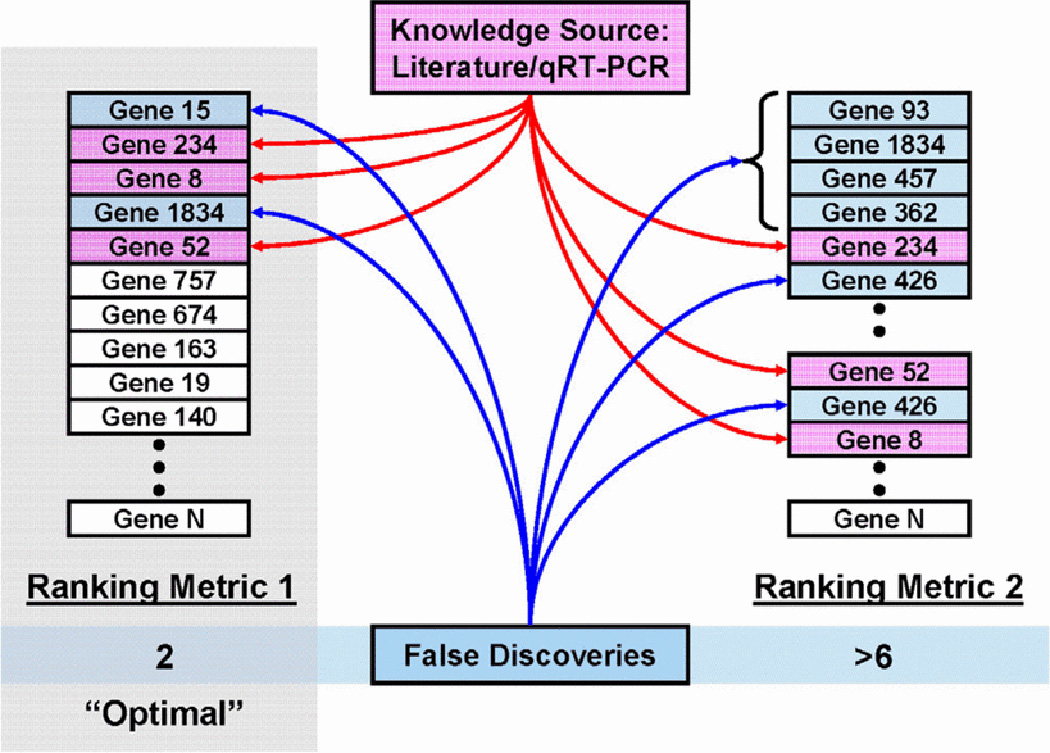
Previously validated biomarkers serve as references with which to determine the relevance of ranking metrics [2]. In Fig. 1, for example, we assume that several genes (8, 52, and 234) have been previously identified and validated for a clinical problem—i.e., these genes have been verified as differentially expressed between the disease conditions of interest. Among the multiple feature ranking metrics, the “optimal”, or most biologically relevant metric, should favorably rank these genes while simultaneously reducing the number of false discoveries (or genes that are not in our knowledge set). However, because our knowledge set is unlikely to be comprehensive, we can usually expect that some of the false discoveries may actually validate as biologically relevant genes. By using the most biologically relevant ranking metric, we increase the probability that these false discoveries, with respect to the current knowledge set, are actually relevant biomarkers. This increased probability leads to an improvement in the efficiency of identifying and validating new biomarkers that we can iteratively add to our knowledge set [2].

Figure 1.

Selection of a biologically relevant ranking metric using existing biological knowledge. The “optimal” method (Ranking Metric 1) minimizes the number of false discoveries with respect to the current knowledge set.

In the following sections, we describe the architecture of omniBiomarker and review the underlying knowledge-based methodology. Using these methods, we optimize the gene ranking metric with respect to prior biological knowledge and identify some novel genes for validation as potential biomarkers for renal cancer subtype classification.

SECTION II. Methods

A. OmniBiomarker Application Architecture

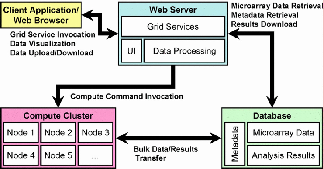
OmniBiomarker contains four components: client, web server, database, and compute cluster (Fig. 2). The client component, or web interface, allows users to interact with the application, relaying input to the web server. The web server component, in addition to responding to user commands and generating the appropriate user interfaces, contains utilities for uploading and downloading data—e.g., gene expression data and gene ranking results—to and from the MySQL relational database. The database component is accessed by both the web server and computation components. Fig. 3 is a simplified representation of the relational database. The computation component receives commands directly from the web server component through a web service and contains parallel-processor utilities for efficiently ranking genes.

Figure 2.

The omniBiomarker application contains four components: the client application (the web browser), the web server, the compute cluster (composed of several nodes, or processors), and the relational database.

Figure 3.

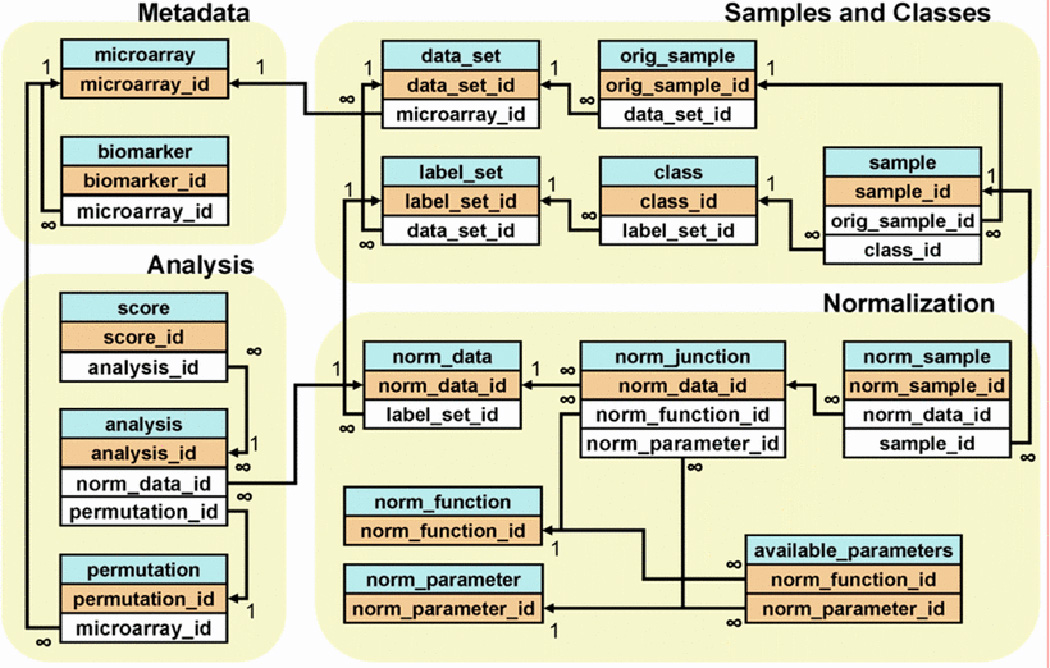
The omniBiomarker relational database is designed to store microarray data as well as gene ranking results. Microarray data are stored in a hierarchy that allows users to pre-process data and assign samples into classes for supervised analysis. The ‘analysis’ table stores all parameters for a particular gene ranking analysis as well as the ranking results (linked with the ‘score’ table) so that users may assess the results from multiple ranking analyses and select the most biologically relevant result.

The relational database organizes information about gene expression values as well as gene ranking results (Fig. 3). Microarray samples—each of which contains expression values for thousands of genes—reside in a multi-level hierarchy that maximizes the flexibility of data analysis and reduces the overall storage requirements. A dataset typically consists of several microarray samples partitioned into specific phenotypic classes. The omniBiomarker interface allows users to customize these sample partitions—called ‘label sets’ in the database—depending on the particular clinical problem. Each gene expression dataset links to metadata tables that contain annotation information for each biomarker. The database also includes several tables that store gene ranking results and analysis parameters.

B. Gene Ranking and Biological Relevance

For a clinical problem, we choose the most biologically relevant ranking metric from among several filter- and wrapper-based ranking algorithms [3]. The filter metrics include the commonly used t-test, fold change, and significance analysis of microarrays (SAM) [4]. The wrapper-based metrics include support vector machines (SVM), signed distance functions (SDF), and linear discriminant classifiers (LDA) [5][6][7]. Wrapper-based metrics rank genes by estimated classification error. Smaller classification error indicates that the gene may be a good predictive biomarker. Because microarray datasets usually have a limited number of samples, we estimate the classification error of each gene using 100 iterations of 0.632+ bootstrap [8][9]. Although we assess several ranking metrics, we only use the single most biologically relevant metric to select candidate biomarkers for validation. The use of multiple metrics also allows us to illustrate the sensitivity of candidate biomarker lists to the selection of a ranking metric.

We compute the biological relevance of each ranking metric with respect to prior knowledge in the form of previously validated biomarkers. A gene ranking metric assigns to each gene, $i$, a score based on its differential expression, $\alpha_{i}$, where $i=1\ldots m$, and $m$ is the total number of genes in a dataset. We assume that lower ranking scores indicate higher differential expression and that all scores are constrained to be within the interval [0],[1]. We define $G_{k}=\{g_{1},g_{2},\ldots,g_{k}\}$ as the set of $k$ relevant biomarkers such that elements of the set $\{\alpha_{i}:i\in G_{k}\}$ are generally smaller than those of $\{\alpha_{j}:j\not\in G_{k}\}$. Genes in $G_{k}$ should be ranked more favorably than the genes that are not in $G_{k}$. We define the following function as the biological relevance of a gene ranking metric, $\theta$:

$$\varphi (G_k,\theta )=\frac{1}{k(m-k)}\sum _{i\in G_k}\sum _{j\notin G}I({\alpha }_i<{\alpha }_j)$$

where $I(x)$ is the indicator function, evaluating to one when $x$ is true and zero otherwise. This formula for biological relevance is equivalent to the area under an ROC curve. The notation presented here is similar to that used in a previous study that examined the biological relevance of gene ranking [2][10][11].

Because we have a limited set of knowledge genes, we use a bootstrap simulation to examine the effect of ranking metric selection on biomarker detection efficiency. The simulation iteratively identifies the most biologically relevant ranking metric using only a subset of the total $K$ knowledge genes—selected by randomly choosing $K$ genes with replacement—then assesses the ability of that ranking metric to detect the remaining knowledge genes. The optimal ranking metric, $\hat{\theta}$, maximizes the likelihood (ML estimation, or MLE) of the biological relevance formula: $\hat{\theta}=\arg{\max}_{\theta}\phi(G_{k},\theta)$. After identifying $\hat{\theta}$ given a subset of the knowledge genes, the simulation ranks all remaining genes, searches for the next biologically relevant gene (possibly encountering some false discoveries), updates the knowledge set, and repeats the process until all genes in $G_{k}$ have been identified. The total number of false detections encountered during this process is inversely proportional to the biomarker detection efficiency. Plotting the biomarker detection efficiency curve (by stepping along the x-axis for each gene encountered during the search and stepping along the y-axis for each correct gene detection) reveals that the area under this curve (AUC) is proportional to the biomarker detection efficiency [2].

C. Clinical Case Study

In the clinical case study, we use a renal cancer dataset derived from a study by Schuetz et al. that uses Affymetrix microarrays (HG-Focus, 8793 probesets) to profile samples from several subtypes of renal tumors, including 13 clear cell (CC) renal cell carcinoma (RCC) and 5 papillary (PAP) [12]. We are interested in biomarkers that differentiate the CC class from the PAP class. Few reliable biomarkers have been validated for this differential diagnosis in clinical practice. We identify biomarkers with qRT-PCR validation and use these biomarkers as knowledge genes to compute biomarker detection efficiency and to propose novel biomarkers that may accurately classify CC and PAP samples. The use of qRT-PCR improves the quality of our knowledge set due to its high sensitivity and specificity.

SECTION III. Results and Discussion

A. Validated Reference Genes

As described in the methods, we identify several biomarkers that are differentially expressed according to qRT-PCR validation (Table 1). We filter qRT-PCR validated biomarkers such that their estimated classification errors are less than 20%. The use of qRT-PCR validated biomarkers increases our confidence in the differential expression of the biomarkers and ensures the quality of our knowledge set [2][13].

Table 1.

qRT-PCR validated genes differentially expressed between the CC and PAP renal cancer subtypes.

Gene Symbol	Error	Gene Symbol	Error
STC1	0.0345774	B3GNT4	0.138581
NDUFA4L2	0.0379203	GRB7	0.168125
CA9	0.0701198	BAMBI	0.169147
CP	0.0781111	CCL20	0.188437
ELF3	0.0819628	CTSC	0.192068
BST2	0.112016	PECAM1	0.194247

B. Gene Detection Efficiency

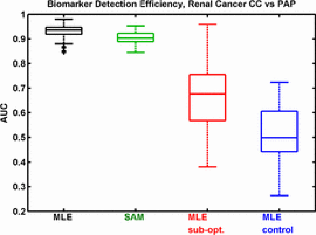
Using our knowledge derived from qRT-PCR experiments, we examine the effect of optimizing the feature ranking metric using the previously described simulation method [2]. For the CC vs. PAP subtype comparison, box plots representing 100 iterations for each test indicate that the knowledge guided feature ranking metric (Fig. 4, black)—selected using the maximum likelihood estimation (MLE) method—outperforms the standard significance analysis of microarrays (SAM, Fig. 4, green) filter method. Furthermore, the quality of the initial knowledge set affects biomarker detection efficiency (Fig. 4, red)—the suboptimal knowledge set is randomly chosen from the total set of genes. As expected, the control test (Fig. 4, blue), in which we are detecting randomly selected genes using randomly selected initial knowledge, results in AUCs of approximately 0.5. This indicates that none of the gene ranking metrics favors uninformative genes better than random chance. Thus, the selection of a ranking metric as well as the quality of knowledge genes (which affects the selection of a ranking metric) affects the biological relevance of gene ranking.

Figure 4.

Area under the curve (AUC) plots representing biomarker detection efficiency for several feature ranking metrics. A larger AUC indicates higher detection efficiency. The optimal ranking metric, selected using maximum likelihood estimation (MLE), is more efficient compared to significance analysis of microarrays (SAM), a standard ranking method. The use of sub-optimal knowledge (sub-opt) when selecting the ranking metric decreases detection efficiency. When using randomly selected genes as knowledge, detection efficiency is random (control).

C. Proposed Genes for Further Validation

Results indicate that the use of biological knowledge to select an optimal gene ranking metric increases the efficiency of detecting additional biomarkers. Using all knowledge genes from Table 1, we identify a single, biologically relevant gene ranking metric. We then used this metric to identify additional genes for validation. Table 2 lists the top 16 genes identified after ranking with the optimal metric, excluding genes previously identified in Table 1. These genes, in general, have not been described previously as RCC biomarkers. However, several have potential relevance for renal tumor pathobiology. For example, synaptopodin (SYNPO) and transcription factor 4 (TCF4) are over-expressed in CC-RCC. SYNPO is expressed in glomerularpodocytes in the kidney and appears to be regulated by vascular endothelial growth factors (VEGF) [14]. Differential VEGF expression is a known feature of the CC subtype [12]. TCF4 is a key participant in WNT pathway signaling, which is dysregulated in several types of cancer. Insulin-like growth factor binding protein 6 (IGFBP6) and glioblastoma amplified sequence (GBAS) are over-expressed in PAP-RCC. IGF binding proteins are biomarkers for several types of cancer [15]. GBAS is a likely target for tyrosine kinases that is co-amplified in some cancers with epidermal growth factor receptor (EGFR) [16]. GBAS is mapped to chromosome 7p12, which is commonly amplified in PAP-RCC [17]. Because we identified these genes using an optimal biologically relevant ranking metric, they are more likely to be true positives. Thus, after qRT-PCR validation, we may add these biomarkers to our knowledge set and iteratively identify additional biomarkers.

Table 2.

Differentially expressed genes between renal cancer CC and PAP subtypes proposed for further validation.

Gene Symbol
IGFBP6	DLG1	TCF4	GABRE
EDNRA	LRRFIP2	DSG2	COL5A2
MYLK	GBAS	ELAC2	RAB4B
INPP5D	SYNPO	HRH1	BIN1

SECTION IV. Conclusion

Biomarkers are essential for the successful treatment of cancer since they enable early detection of the disease before significant symptoms arise. Moreover, pathologists may use biomarkers to acquire information about disease prognosis from tissue biopsies that may not be readily apparent using traditional staining techniques. A cancer detection screening using biomarkers is essentially a clinical predictor that assigns patients to categories of disease presence/absence or degree of disease severity. Accurate assignment of patients into these categories will enhance therapeutic efficacy and improve treatment success rates. However, biomarker identification is difficult because of the large technical and biological variability of the data. Many gene ranking and selection methods exist, each of which may produce different results. In this paper, we have presented an emerging translational bioinformatics method that uses prior biological knowledge to guide ranking algorithm selection. By using the most biologically relevant ranking metric, we increase the efficiency of identifying novel biomarkers and decrease the false discovery rate. These knowledge-guided methods are encompassed within a web-based bioinformatics application called omniBiomarker. As a case study, we applied these methods to a renal cancer dataset and identified novel biomarkers.

REFERENCES

- 1.Somorjai R, Dolenko B, Baumgartner R. Class prediction and discovery using gene microarray and proteomics mass spectroscopy data: curses caveats cautions. Bioinformatics. 2003;19(12):1484–1491. doi: 10.1093/bioinformatics/btg182. [DOI] [PubMed] [Google Scholar]
- 2.Phan J, Yin-Goen Q, Young A, Wang M. Improving the Efficiency of Biomarker Identification Using Biological Knowledge. 14:427–438. [PMC free article] [PubMed] [Google Scholar]
- 3.Xiong M, Fang X, Zhao J. Biomarker Identification by Feature Wrappers. Genome Research. 2001;11:1878–1887. doi: 10.1101/gr.190001. [DOI] [PMC free article] [PubMed] [Google Scholar]
- 4.Tusher V, Tibshirani R, Chu G. Significance analysis of microarrays applied to the ionizing radiation response. PNAS. 2001;98(9):5116–5121. doi: 10.1073/pnas.091062498. [DOI] [PMC free article] [PubMed] [Google Scholar]
- 5.Cristianini N, Shawe-Taylor J. An Introduction to Support Vector Machines and other Kernel-based Learning Methods. Cambridge University Press; 2000. [Google Scholar]
- 6.Boczko E, Young T. The signed distance function: a new tool for binary classification. 2005 arXiv:cs.LG/0511105vl. [Google Scholar]
- 7.Cheng C-C, Lin C-J. LIBSVM: a library for support vector machines. 2001 [Google Scholar]
- 8.Efron B, Tibshirani R. Improvements on Cross-Validation: The .632+ Bootstrap Method. Journal of the American Statistical Association. 1997;92(438):548–560. [Google Scholar]
- 9.Braga-Neto U, Dougherty E. Is cross-validation valid for small-sample microarray classification? Bioinformatics. 2004;20:374–380. doi: 10.1093/bioinformatics/btg419. [DOI] [PubMed] [Google Scholar]
- 10.Phan J, Young A, Wang M. Selecting Clinically-Driven Biomarkers for Cancer Nanotechnology. :3317–3320. doi: 10.1109/IEMBS.2006.259746. [DOI] [PubMed] [Google Scholar]
- 11.Mukherjee S, Roberts S. A theoretical analysis of the selection of differentially expressed genes. J Bioinformatics Comput Biol. 2005;3:627–643. doi: 10.1142/s0219720005001211. [DOI] [PubMed] [Google Scholar]
- 12.Schuetz AN, Yin-Goen Q, Amin MB, Moreno CS, Cohen C, Hornsby CD, Yang WL, Petros JA, Issa MM, Pattaras JG, Ogan K, Marshall FF, Young AN. Molecular Classification of Renal Tumors by Gene Expression Profiling. J Mol Diagn. 2005 May;7(2):206–218. doi: 10.1016/S1525-1578(10)60547-8. [DOI] [PMC free article] [PubMed] [Google Scholar]
- 13.Chuaqui R, Bonner R, Best C, Gillespie J, Flaig M, Hewitt S, Phillips J, Krizman D, Tangrea M, Ahram M, Linehan W, Knezevic V, Emmert-Buck M. Post-analysis follow-up and validation of microarray experiments. Nature Genetics. 2002;32:509–514. doi: 10.1038/ng1034. [DOI] [PubMed] [Google Scholar]
- 14.Ostalska-Nowicka D, Zachwieja J, Nowicki M, Kaczmarek E, Siwinska A, Witt M. Vascular endothelial growth factor (VEGF-C 1)-dependent inflammatory response of podocytes in nephrotic syndrome globerulopathies in children: an immunohistochemical approach. Histopathology. 2005;46(2):176–183. doi: 10.1111/j.1365-2559.2005.02076.x. [DOI] [PubMed] [Google Scholar]
- 15.Fu P, Thompson J, Bach L. Promotion of cancer cell migration: an insulin-like growth factor (IGF)-independent action of IDF-binding protein-6. Journal of Biological Chemistry. 2007;282(31):22298–22306. doi: 10.1074/jbc.M703066200. [DOI] [PubMed] [Google Scholar]
- 16.Segditsas S, Tomlinson I. Colorectal cancer and genetic alterations in the Wnt pathway. Oncogene. 2006;25(57):7531–7537. doi: 10.1038/sj.onc.1210059. [DOI] [PubMed] [Google Scholar]
- 17.Wang X, Smith D, Liu W, James C. GBAS a novel gene encoding a protein with tyrosine phosphorylation sites and a transmembrane domain is co-amplified with EGFR. Genomics. 1998;49(3):448–451. doi: 10.1006/geno.1998.5239. [DOI] [PubMed] [Google Scholar]