A genome-wide approach for detecting novel insertion-deletion variants of mid-range size

Abstract

We present SWAN, a statistical framework for robust detection of genomic structural variants in next-generation sequencing data and an analysis of mid-range size insertion and deletions (<10 Kb) for whole genome analysis and DNA mixtures. To identify these mid-range size events, SWAN collectively uses information from read-pair, read-depth and one end mapped reads through statistical likelihoods based on Poisson field models. SWAN also uses soft-clip/split read remapping to supplement the likelihood analysis and determine variant boundaries. The accuracy of SWAN is demonstrated by in silico spike-ins and by identification of known variants in the NA12878 genome. We used SWAN to identify a series of novel set of mid-range insertion/deletion detection that were confirmed by targeted deep re-sequencing. An R package implementation of SWAN is open source and freely available.

INTRODUCTION

Structural variants (SVs) include insertions and deletions (indels) as well as other genomic rearrangements such as inversions, duplications and transpositions. SVs have significant phenotypic implications that can increase the susceptibility to a variety of diseases (1,2). Paired-end next generation sequencing (NGS) of whole genome shotgun (WGS) libraries is currently the most commonly used method for discovering SVs. However, even with the technological advances in NGS, the discovery and accurate characterization of SVs has faced significant challenges compared to the discovery and genotyping of single nucleotide variants (SNVs). SVs display a broad range of categories (insertions, deletions, duplications, etc.) and sizes, and SV discovery is inherently more susceptible to sequencing and mapping artifacts in WGS data.

As shown in an independent comprehensive benchmark by Blue Collar Bioinformatics (http://bcb.io) (3), and as we demonstrate in our own comparison studies, current SV detection methods lack sensitivity for the detection of smaller deletions, insertions and other complex variants. However, this class size of SVs is among the most frequently occurring in the genome, as determined by local assembly and deep sequencing (4). Even more challenging is the detection of SVs that are heterozygous or present at low allelic fractions for a given sample. The latter case commonly occurs in cancer samples due to genetic heterogeneity and somatic mosaicism (5,6).

To address these challenges in SV detection, we developed a systematic approach that improves sensitivity and precision over current methods, especially for detecting insertions and small deletions. We refer to our method as Statistical Structural Variant Analysis for NGS (SWAN). Herein, we demonstrate that this approach has significantly improved sensitivity for indel detection (50 bp–10 Kb), especially in heterozygous cases and cases where the variant occurs at a reduced fraction in mixed genetic samples.

SWAN leverages a combination of mapping features in WGS data that are caused by structural variation junctions. These features include (i) local change in coverage, (ii) change in mapped insert size, (iii) clipped or split reads and (iv) hanging read pairs. By leveraging all of these features simultaneously, SWAN achieves superior sensitivity through a comprehensive statistical framework that aggregates evidence over all informative read-pairs and all mapping signatures in the detection of each variant. SWAN's probabilistic model focuses on detecting sequence insertion and deletions. Because sequence insertions and deletions are elements of more complex SVs, SWAN can also detect classes of SVs beyond simple insertion and deletions (see Supplementary Figure S1). SWAN combines the information from all mapping features through the computation of likelihood ratio scan statistics of Poisson random field models.

Most methods for detecting SVs from WGS data rely heavily on one feature, and none employ a full probabilistic model for local background adjustment. For example, the 1000 Genomes Project (7) employed a series of SV detection algorithms that rely on only one or two signal features. CNVnator (8) uses coverage, BreakDancer (9) uses insert size, both Pindel (10) and Delly (11) use a combination of insert size and split reads. GASVPro (12) uses both coverage and insert size information. A newer algorithm, Lumpy (13), also uses insert size and split reads. We show that, by leveraging multiple signal features in combination with a statistical model that adjusts for the background distribution, SWAN achieves higher sensitivity, precision and a broader detection spectrum compared to other methods. Most importantly, we identified a series of mid-range sized indels that were previously not identified by WGS analysis with other SV callers.

The underlying principles of SWAN were initially described as a purely mathematical derivation of these scan statistics with a description of rigorous false discovery rate control and power analysis (14). The focus of this current study is the implementation and application of a complete bioinformatics process to identify medium range indels from both in silico and real whole genome sequencing data. We describe a novel set of mid-range indels that have not been identified previously and independently verified their structure with targeted re-sequencing.

MATERIALS AND METHODS

SWAN workflow

Figure 1A provides an overview of SWAN analytical process with three distinct stages: (i) empirical estimation of library-specific parameters (Figure 1B); (ii) whole genome scans of multiple mapping features to identify candidate regions (Figure 1C and D); and (iii) joining of evidence and merging of signals. The genome-wide scan consists of two modules: a likelihood ratio-based scan module and a soft-clip/split read remapping module. These processes can be easily adapted for compute parallelization. The likelihood-scan (Figure 1C) computes likelihood-ratio scan statistics based on inhomogeneous Poisson field models for the coverage (), the mapped insert size of read pairs () and upstream and downstream hanging pairs (). The soft-clip/split read module (Figure 1D) aggregates and remaps clusters of soft-clip/split reads.

Figure 1.

SWAN framework. (A) General workflow. (B) SWAN applies robust and library-aware statistics to enable multi-library analysis: top left, a perfect library distribution with insert size mean I, density and distribution ; top right, a heavily skewed insert size distribution and SWAN fit of mean, right density and left density; bottom left, a double mode library with high kurtosis and heavy left tail with SWAN fits; down right, a multiple library combination where SWAN fits a separate density to each library. (C) Four types of mapped paired-end reads (MPRs) in the vicinity of a window containing a putative deletion (for insertions, w = 0). These MPRs are used to construct the likelihood ratio scan statistics as in Table 1. (D) Reciprocal remapping procedure for soft-clipped reads. (E) A more detailed workflow for SWAN.

At the evidence joining stage, SVs are detected by scanning for ‘peaks’ in the likelihood ratio tracks, combining overlapping peaks and integrating these locations by soft-clip/split read cluster remapping. One can control the false discovery rate (FDR) by setting the thresholds for calling peaks. When the data are noisy, we have implemented SWAN such that the thresholds are automatically set at more stringent level. At the end of the processing, SWAN merges the potential calls by weighting the joined evidence and carrying forward the most supported ones. This stage is very fast, and since intermediate results are saved, the user can experiment with thresholds of varying stringency.

An essential step to accurate SV discovery involves estimating the insert size distribution of the sequencing libraries, which is often heavily skewed and sometimes multi-modal. Most software assumes a normal distribution, but in these cases, it is a poor fit to the data. In SWAN, the library parameters are estimated using a robust approach that minimizes the effects of skewness and multimodality. When multiple libraries of different read lengths and insert-size distributions are sequenced for a given sample, SWAN estimates the parameters for each library separately and combines the reads across libraries by summing their library-specific likelihoods. Figure 1B shows several examples of how SWAN fit multi-library models and estimate library-specific parameters given complicated input distributions. The details of SWAN insert size fitting are described in Supplementary Text S1.

SWAN is implemented as an open source R and C++ package. Supplementary Figure S2A shows a single sample analysis for germ-line variants and Supplementary Figure S2B shows a paired analysis of tumor and control samples for somatic variants. These analysis pipelines are all demonstrated in examples that accompany the software package. The confidence in the boundaries of a structural variant detection depends on the mapping features that led to its detection. Exact boundaries and genotypes are determined based on soft-clip/split read analysis whenever possible. SWAN source code and manuals are available at http://bitbucket.org/charade/swan.

Generalized likelihood ratio scan framework for SWAN

The likelihood ratio scans in SWAN are comprised of four separate processes , , , each derived from a generalized likelihood ratio. First, we specify the background (null) model (14) for the WGS data, which applies to the case where the sample is identical to the reference genome. In the background model, the positions of mapped paired-end reads are sampled as follows; (i) the position of the first read, u, is sampled via a Poisson process; (ii) the position of the second read, v, is equal to u+I, where I, the insert size, is sampled from a known distribution f_I. Either u or v can be missing due to sequencing or mapping error, with probability p, in which case the read pair is said to have a hanging end. We let be the inhomogeneous rate of reads mapping to genome position .

Full theoretical derivations, found in (14), lead to the representation of this model as a Poisson random field on , where G is the reference genome, with rate function of the form

(1)

Here, and is the mean coverage process under the null hypothesis. Thus, the Poisson rate for a read pair (u,v) depends on the local coverage and , the mapped insert size and whether one of the reads is hanging.

The Poisson distribution is a good approximation of shotgun-sequencing data and has numerous applications (15). Overdispersion relative to the Poisson is often observed in NGS data, particularly in RNA-Seq settings (16). Empirically, sequence features such as GC-content bias explain some of the overdispersion, and the negative binomial distribution has been suggested as a better model for the data (17,18). By directly modeling and accounting for the inhomogeneity in the underlying mean process κ of the Poisson field, we alleviate the overdispersion issue; that is, with the mean adjusted to reflect local fluctuations, the Poisson distribution is a simple and effective model for the local read pair count.

The parameters of the process are estimated empirically in stage I of scan: the mean process κ is computed by smoothing the base-wise coverage process. The insert size distribution is estimated as described in Supplementary Text S1. The hanging read probability p is estimated by the percentage of hanging read pairs among all read pairs.

Next, we examine changes to this Poisson field in the presence of a SV. We consider the example of a genomic deletion; insertions follow a similar model. All mapped read pairs (MPR) within the neighborhood of a deletion of size w fall into four categories (Figure 1C): (i) Insider MPRs, denoted by S^W, have at least one read overlapping the deleted segment, e.g. MPR1 in Figure 1C. Essentially, this class of read pairs overlap directly with the hypothetical SV region. (ii) Spanning MPRs, denoted by S^C, have one read mapping downstream and the other read mapping upstream of the SV, e.g. MPR2 in Figure 1C. These read pairs straddle the hypothetical region. (iii) Up-anchoring MPRs, denoted by S^U, have one read mapping upstream from the SV anchoring a hanging read that fails to map, e.g. MPR3. (iv) Down-anchoring MPRs, denoted by S^D, are the same as up-anchoring MPRs, but with the anchoring read mapping downstream from the SV, e.g. MPR4.

Now, we derive the likelihood ratio scan statistics. We first hypothesize that there is a w-bp structural variant (w > 0) starting at the reference position s (for insertions, w = 0). Then, in the vicinity of the hypothetical SV window [s, s+w], as shown in Figure 1C, we expect the rate λ(u, v) of the Poisson field for MPRs to change in ways that are specific to the size, type and allele frequency of the variant. The allele frequency r can be understood as the fraction of chromosomes carrying the variant in the DNA mixture. The hypothesis tests for which we compute generalized likelihood ratios are

(2)

Below, we show how we derive the likelihood ratio statistics , , for testing H₁ versus H₀ using each of the four categories of MPRs.

Likelihood ratio scan for insider MPRs

The signal compares the coverage within to background local coverage. We define the insider MPRs set: , which all have at least one read overlapping with the putative SV window W. For a w-sized deletion , while for a w-sized insertion at s, , since the inserted sequence is not observable using reference coordinates. Given a SV, the coverage within W is expected to decrease to of its expected null coverage. In other words, the term changes to in Equation (1) for any . The log-likelihood ratio statistic to capture the signal from insider MPRs can easily be derived from the Poisson distribution:

(3)

where and for any event E, I(E) is the indicator function for E being true. Intuitively, this Poisson-derived log-likelihood is a weighted window coverage, with each base in the window weighted by the inhomogeneous coverage function κ. The last term penalizes for the size of the window.

Likelihood ratio scan for spanning MPRs

The signal compares the mapped insert size of read pairs spanning to the global insert size distribution. This set of MPRs is denoted by . When a MPR comes from a fragment containing a w-sized deletion, its inferred insert size will be w larger than the true size of the fragment. Thus, MPRs from fragments containing deletions behave as if being sampled from insert size distribution instead of the null distribution . Similarly, if the MPR spans an insertion of size w, its expected insert size would be w smaller than the null expectation, and thus the alternative insert size distribution would be . For a variant present at mixture fraction r, a fragment has probability r of spanning the variant. To simplify notation, we let and allow w to take negative values for w-sized insertions. For MPRs that span the genomic segment of interest, Equation (1) and its rate function are altered by replacing with . The log likelihood ratio scan statistic for deletions and insertion from MPRs in , from (13), is of the form

(4)

The term compares the likelihood of the insert-size y_i under the alternate hypothesis (where there is a deletion of size w) to its likelihood under the null. For a given value z, the function dampens smaller values of z toward zero, thus reducing noise. Intuitively, this scan statistic sums over the spanning read pairs a denoised likelihood term reflecting the deviation of the insert-sizes from the mean.

Likelihood ratio scan for hanging (anchoring) MPRs

The signal compares the rate of hanging pairs immediately upstream of s to the background rate, while the signal compares the rate of hanging pairs immediately downstream of s + w to the background rate. We define hanging MPRs (SAM flags: 73, 137, 121, 185, 105, 169, 89, 153) as read pairs having only one mate anchoring within distance Δ (down/up stream) from the SV window W:

where N.A. means mapping position unavailable (i.e. the read is unmapped). Due to the difficulty of mapping sequence reads across SV boundaries, both insertion and deletions are expected to generate hanging MPRs belonging to (S^U) and (S^D). The likelihood for an MPR in S^U or S^D under the alternative that there is an SV at [s, s + w] at proportion r in the sample depends on the distance of the mapped read to the boundary. For example, an MPR (u, N.A.) in S^U can be generated in two ways: from a reference template, with the hanging read due to error, or from a variant, in which case the hanging read may be due to error or to its overlap with a deletion boundary or inserted sequence. The rate for the former event is (1 − r)λ(u, v) and the rate for the latter event is , where F_I is the cumulative distribution function of f_I and R is the read length. In Equation (1), given the unknown value of κ for new sequence generated by an SV, we substitute it with the average value .

Intuitively, the new rate function has higher probability value for observing hanging read pairs, if the distance of the mapped mate from the putative SV boundary is probable under the known insert size distribution. Letting x_i be the non-missing value of and R the read length, the overall log likelihood ratio statistic to detect deletions for MPRs in is

(5)

Similarly, the overall log likelihood ratio contribution from MPRs in :

(6)

The corresponding statistics to detect insertions are similar. See Supplementary Text S1 and (14) for more details regarding this likelihood process.

Joint whole genome scan and SV detection algorithm

To enable efficient and rapid computation, SWAN carries out a joint genome-wide scan using all likelihood ratio processes for and with a small step size b (default value of b is 10 base pairs). SWAN requires input of parameters w and r. While w and r are generally unknown and take on different values for different instances of SV across the genome, we known from simulations that the power of the generalized likelihood ratio statistics are only weakly dependent on assuming the correct values of w and r (14). For example, if we set w = 20 and r = 0.1, the scan maintains good sensitivity when the actual deletion size is larger than 20 bp and the actual mixing fraction is larger than 10%.

In (14), we demonstrated a method to compute thresholds for L^t that controls the false positive rate at a given Type-I error α for likelihood ratio scans on Poisson fields. SWAN computes these thresholds instantaneously using the estimated library parameters and scan settings (r, w, b). After the joint genome-wide scan finishes, we collect the statistically significant positions , where and is the local threshold for the corresponding feature that controls Type-I error α.

Subsequently, the significant regions detected by , and are combined with detections made simultaneously by and as follows: First, overlapping 's and 's are joined and merged to form deletion calls. Second, we define a pair of hanging read signals as a telescoping pair if they are within m bases apart, which by default is three times the insert size standard deviation . This type of telescoping pair is produced when a short insertion or deletion is contained between and . Detections by and are made by taking all such telescoping pairs. In our experience, the hanging read scores are often noisy and a telescoping pair of hanging read signals is much more reliable than a singleton peak.

We describe the indel detection process. A region is reported to contain a putative deletion if it contains a coverage signal , a spanning pairs signal or a telescoping pair of hanging reads signals and . A region is reported to contain a putative insertion if it contains a spanning pair's signal or a telescoping pair of hanging read signals and . The set of putative deletion and insertion regions can are then compared to the soft-clip/split read remapping results for breakpoint confirmation, as illustrated in Figure 1E. The inversion events are detected in similar fashion as the insertions because they also generate breakpoints and de novo sequence insertions.

Soft-clip and split read clustering and remapping

Soft-clip and split sequence reads resulting from mapping issues that occur downstream and/or upstream flanks (i.e. ‘tips’); clipping of the sequence occurs because of mismatches with the reference. Depending on the size of the clipped portion of the read and the aligner, the tips may or may not have a secondary alignment (i.e. leading to a split read). When there is a low background clip rate, soft-clip/split reads offer evidence of break point location and variant type. In SWAN, clusters of soft-clipped reads are used in two ways. (i) SWAN brackets the left-clip and right-clip clusters as possible evidence for insertions or inversions. (ii) SWAN brackets pairs of soft-clip clusters and uses this information to identify SV breakpoint junctions by remapping the consensus clipped sequences.

SWAN's soft-clip/split read scan has two stages. In the first stage, it identifies all soft-clip/split read clusters that have more than c reads and d bases clipped at the same position and orientation (upstream/downstream) with the clipped sequence forming a consensus. The thresholds are chosen based on taking the maximum between the top percentile of the genome and the top percentile of the local 10 Kb region. We call these clusters left (right) clusters if they are up (down) stream clipped. In the second stage, SWAN remaps the consensus sequence of these clusters to the reference, and then screens for a pattern that we call reciprocal mapping, as illustrated in Figure 1D. In reciprocal mapping, the clipped consensus of one cluster is mapped directly adjacent to another cluster and the clipped consensus of the other cluster maps back to the initiating cluster. Such reciprocal mapping gives us highly confident and precise SV boundaries.

Depending on the data quality, a relatively small fraction of soft-clip clusters may achieve reciprocal mapping. To improve sensitivity for insertions, SWAN scans the remaining clusters for left and right cluster pairs that are within a half read length of each other. These putative insertion points are combined with likelihood ratio peaks as putative insertion signals.

Benchmark data sets and validation of novel SVs

Simulated data sets

We generated simulated Illumina WGS data sets (e.g. BAM files), spiking into the human reference genome (hg19) 15 000 SVs including deletions, insertions, inversions, duplications and transpositions of varying sizes. We used SVEngine (http://bitbucket.org/charade/svengine), BWA-MEM aligner (19) and SAMtools (20) to simulate the data sets. One set of data had average sequencing coverage ranging from 5X to 50X with 100% SV allelic fraction. The other data set had 50X coverage with from 5% to 100% in SV allele fractions with 50X coverage.

With the simulated BAM file input, we benchmarked SWAN along with CNVnator (21), BreakDancer (9), Delly (11), Lumpy (13) and Clever (22). These benchmarked methods are chosen because they are representative of a general category of SV detection approaches. For instance, the Phase One portion of the 1000 Genomes Project (23) utilized several SV methods – CNVnator (21), BreakDancer (9) and Delly (11), which used coverage, insert size, soft-clip/split reads or a combination of the latter two, respectively. Also, we included Lumpy (13), which combines the latter two signals, and Clever (22), which is designed to detect small to mid-range deletions.

There are many other SV calling methods exist that include the following: ReadDepth (24), RDXplorer (25) and CNVeM (26), which use read depth; VariationHunter (27), PEMer (28), HYDRA (29) and MoDIL (30), which use insert size; and AGE (8), ClipCrop (31) and CREST (32), which use hanging reads, split read remapping and soft-clipped reads respectively. These other programs rely on sequence features that overlap with the SV callers that we compared with SWAN. Testing all SV detection methods was impractical so we focused on those that were representative of specific categories of detection methods.

Using our in silico data set, we compared each method's overall performance based on recall, precision, accuracy (F1-measure) and FDR. We refer the readers to Supplementary Text S1 for the details of simulation process, program parameters and performance measuring.

Platinum genome data sets

We compared the performance of SWAN with other methods on the WGS sequence data of NA12878 from the Illumina Platinum Genomes project (ENA Accession: ERP001960). Two previously curated validated deletion sets are available for this sample, one based on PCR amplicon confirmation of breakpoints and the other based on long read (LR) sequencing. We compared SWAN's performance to the performance of Pindel (10), Delly (11), GASVPro (12) and Lumpy (13), which are all cited from Layer et al. (13).

Targeted sequencing

To confirm the presence and structure of novel indels detected by SWAN, we used a targeted sequencing technology called Oligonucleotide-Selective Sequencing (OS-Seq) (33), which can accurately characterize candidate SV boundaries with high accuracy (34). The genomic targets for potential breakpoints are shown in Supplementary Table S1. Sequence read pileup tracks from OS-Seq, overlaid on top of the SWAN detection segments, were inspected to validate true positives and determine the precise sequence break points (example snapshots are shown in Figure 2B–D). The OS-Seq sequence data were deposited to NCBI's Short Read Archive (id: SRX1059374).

Figure 2.

Performance benchmark and validation of novel indel calls with Platinum Genome data set (NA12878). (A) Study design of the OS-Seq targeted sequencing validation. (B–D) Genome browser view of pileups plots of validated structural variant regions SWAN novel indel calls not previously identified by literature: (B) a homozygous deletion, (C) a heterozygous deletion and (D) a homozygous insertion.

RESULTS

Benchmark analysis with simulated data sets

The simulated spike-in data allow us to evaluate the accuracy of methods on SVs over a broad category of types, sizes and allelic fractions. Each spike-in sample contains 2500 each of insertions, deletions, inversions, duplications and transpositions, as well as 2500 insertions of random sequences derived from the adenovirus genome (Chimpanzee adenovirus NC_017825.1). We focused primarily on the mid-sized SV events that are smaller than 10 Kbp (8). Details of the procedure details are described in Supplementary Text S1 and the simulated data set is downloadable at http://hamachi.stanford.edu/publication-material/swan/swan-data.tgz).

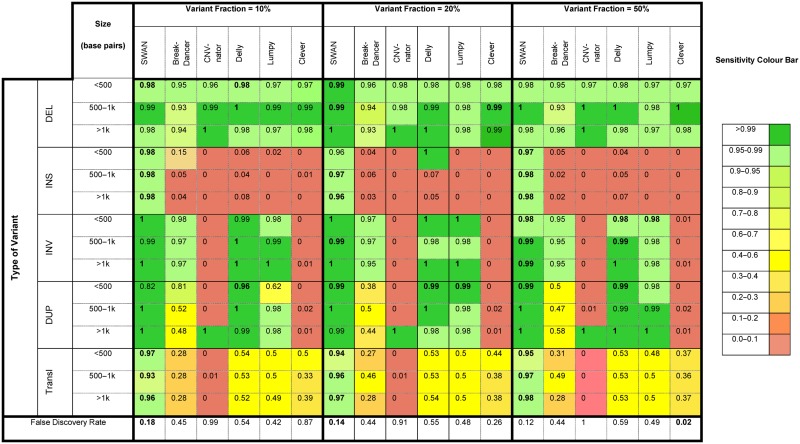
In Table 1 we summarize the sensitivity and FDR of SWAN, Lumpy, Delly, BreakDancer, CNVnator and CLEVER. The cells of Table 1 are colored by the achieved sensitivity for a specific category of SV. The last row of the table shows the FDR of each method. First, SWAN produced fewer false positives compared to the other methods. At this lower FDR, SWAN achieves comparable or improved sensitivity across all variant types, size ranges and allele frequency levels. From this study of simulated SV data, we find that in addition to deletions, SWAN is able to detect insertions, duplications and transposition events reliably, thus complementing the detection spectrums of current methods. SWAN maintains high sensitivity across the spectrum of SV classes due to its integration of multiple types of signals in the whole genome scan, and its use of a probabilistic model for background adjustment. Additional simulation results can be found in Supplementary Table S2 and Supplementary Figure S3, where comparisons were plotted by gradients of SV allelic fractions, coverage and variant sizes.

Table 1. Performance benchmark based on simulated data with spike-in SV events.

The complete pipeline SWAN is more sensitive than simply using any of its single likelihood tracks, each of which is based on only one mapping feature. Detailed benchmark results of SWAN against these single likelihood tracks are given in Supplementary Table S3. For instance, for both homozygous and heterozygous variants of all types smaller than 500 base pairs, SWAN has 96–97% combined sensitivity while the sensitivity from hanging reads alone (L^D/L^U) is 41–42%, from insert-size alone (L^C) is 28%, and from the rest of the features combined (SoftClip, L^W, etc) is 26–27%. The same is true for larger variants and for variants of lower allele-frequency. For example, for variants between 500 base pairs and 1 Kbp of allele frequency (5–20%), SWAN has 96–97% combined sensitivity while the sensitivity from hanging read is 41–43%, from insert-size is 28% and from the rest of signals combined is 26–27%. If one were to focus on SVs of a specific size range, the complete SWAN pipeline using all features remained the most sensitive among the methods tested. However, SWAN's sensitivity is nearly the same when relying on only one feature. For example, for homozygous and heterozygous deletions less than 500 base pairs, SWAN has 98–99% sensitivity while the sensitivity from insert-size alone is also 98–99%. These results show that, by aggregating signals across features, SWAN achieves high sensitivity for more structural variant types, across a broader size range, and under lower allele frequency.

The superior sensitivity achieved by SWAN through feature aggregation does not significantly lower the precision, which is at 86% across all variant types. There is a small reduction in precision when each likelihood track is used as a single metric. Citing an example, for calling homozygous and heterozygous deletions, the insert size (L^C) feature alone achieves a 99% precision, which is higher than SWAN's 86%, but its sensitivity is 28–29% much lower than SWAN's 96–98% (Supplementary Table S3). In summary, the complete pipeline in SWAN significantly increases sensitivity over individual likelihood scans while still maintaining good precision. Simulated sequence data does not fully capture the heterogeneity as seen in real sequence data (which we will address in the analysis of actual WGS). However, these data allow us to systematically evaluate the accuracy of methods across a broad spectrum of settings for a comprehensive set of variants.

Benchmark analysis with platinum genomes

As an additional benchmark, we used SWAN to analyze the WGS data of individual NA12878 from the Illumina Platinum Genomes project. The NA12878 WGS sequence data have been extensively analyzed in other studies. We examined both the original 50X average coverage data as well as a down-sampled set of data with 5X average coverage (20). Layer et al. (13) assembled two sets of deletions that underwent validation in previous studies: 3376 deletions were validated by individual PCR breakpoint amplicon assays (7,23); 4095 deletions that have long read (labeled LR) support from Pacific Biosciences long reads (7).

Using these two validated deletion sets as ground truth, we benchmarked SWAN's performance with other methods, including Lumpy, Delly, GASVPro and Pindel. We computed sensitivity and ‘FDR’. We put quotes on FDR here because detections that are not in the validated deletion set may also be true variants, as we show through additional validation experiments. The performance assessment for Lumpy, Delly, GASVPro and Pindel are previously independently reported by Layer et al. (13).

Table 2 shows the recall proportion on both validated sets, as a measure of sensitivity, as well as the overall FDR, computed from the fraction of detections not found in either validation sets (See Materials and Methods for definition of FDR). At 50X coverage, according to the PCR assay validation set, SWAN has the highest recall of the five programs and the lowest FDR along with GASVPro. According to the long-read validation set, SWAN has the highest recall (along with Delly), and the lowest FDR (along with Lumpy and GASVPro). With 5X coverage, SWAN has a slightly higher FDR and substantially higher sensitivity than the others, with the exception of GASVPro, which has substantially lower FDR and sensitivity.

Table 2. Performance benchmark based on Platinum genomics NA12878 data.

	50x Coverage			5x Coverage
	Sensitivity		‘FDR’	Sensitivity		‘FDR’
	PCR	LR	PCR+LR	PCR	LR	PCR+LR
SWAN	74%	80%	42%	28%	23%	17%
Lumpy	61%	72%	43%	11%	8%	17%
Delly	60%	60%	73%	20%	12%	19%
Pindel	60%	82%	76%	14%	19%	15%
GasvPro	51%	59%	41%	15%	10%	9%

Identifying novel indels

As we previously described, the two validated sets of NA12878 were based on consensus detections reported from published studies (7,23). We examined the true positive rate among a set of SWAN's novel indels that were not among the externally validated SVs including PCR verification and long read sequencing. We chose 138 SWAN novel candidate sites (87 deletions and 51 insertions) for deep targeted re-sequencing (see Figure 2A). To confirm the presence and structure of these novel indels detected by SWAN, we used a targeted sequencing technology called Oligonucleotide-Selective Sequencing (OS-Seq) (33). Previously, we had demonstrated that this method could accurately characterize candidate SV boundaries with high accuracy (34). We limited our study to SVs of size smaller than 500 base pairs, most having sizes in the 100–500 range, because we can validate indels with high confidence in this size range using the OS-Seq targeted re-sequencing.

OS-Seq utilizes target specific primer-probe and oligomer hybridization in a massively parallel fashion to provide ultra-high coverage downstream target sequences (34) within 1 Kb range of the designed primers. We successfully developed up to two primer pairs (one pair is one reverse and one forward strand primer) for 108 candidate SV sites flanking the break points for special OS-Seq targeting assays. For the 108 selected indel candidates, we successfully sequenced 102 (∼95% of 108, including 70 deletions and 32 insertions) with an average coverage of ∼14 000X. Using these data, we sought to resolve the breakpoint boundaries. Those candidate indels (30 sites) which we could not target sequence occurred in highly repetitive regions, thus limiting the on-target selection of flanking sequences around this subset of putative breakpoints (see primer designs in Supplementary Table S1).

With this high depth of coverage, we resolved indel breakpoints with high resolution and confidence. Among this 102 candidates underwent deep-targeted sequencing, SWAN initially identified 70 as deletions and 32 as insertions. Our targeted sequencing validation confirmed 66 (94%) of the 70 deletions and 25 (78%) of the 32 insertions (Table 3). These new indels were missed by the previous studies because of their small size, their heterozygous genotype (Figure 2B–D), and/or the complexity in their structure. For example, we identified two non-reference alleles (see Supplementary Table S1).

Table 3. Summary statistics of OS-Seq targeted sequencing analysis of SWAN calls.

	DEL	INS
Total	70	30
Validated	66	25
Rate	94%	78%

In Figure 2B–D, we show three representative examples of novel SWAN indel discoveries. The first is a homozygous deletion of 53 base pairs (chr1: 175 091 594–175 091 647) catalogued in the database of genomic variants (DGV) (35) (id: nsv160653). As it turns out, this SV was independently validated by sequencing of a fosmid clone as reported by Mills et al. (36). This SV is a common variant with ∼60% frequency in 2504 individuals impacting the intron region of human tenascin N (TNN) gene (37). The second example is a heterozygous deletion of 51 base pair (chr14: 98 822 621–98 822 672). This exact deletion has not been previously catalogued but an overlapping deletion with similar boundaries is registered (id: esv2749092) in DGV. The final example we cite is a homozygous insertion (chr2: 28 163 501–28 163 502) that overlaps with a 34 base pair common insertion detected with ∼81% frequency in 2504 individuals and residing in the intron region of BRE gene. Detailed information of the other OS-Seq validated SWAN novel detections are in Supplementary Table S1.

DISCUSSION

We described SWAN, a new statistical framework and algorithm for SV detection from whole genome sequencing data. SWAN integrates multiple features, including insert size, hanging read pairs and read coverage into one statistical framework and detects putative SVs through genome-wide likelihood ratio scans. SWAN remaps soft-clip/split read clusters to supplement the likelihood analysis, joins multiple sources of evidence and identifies break points whenever possible. SWAN has improved sensitivity for detecting structural variants smaller than 10 kilobases and is particularly successful at identifying deletions smaller than 500 base pairs.

The size range ≤100 bp is where SWAN has the most significant improvement, due to SWAN's careful modeling of the insert size distribution. Indeed, 41 (58%) of the 70 validated SWAN de novo deletion calls fall into this range. The simulation results for spike-ins with sizes in the range ≤100 bp (Supplementary Table S4) show that SWAN has the best sensitivity for insertions, deletions and translocations for variant fractions from 20% and up among all benchmarked callers. In our simulation scenarios SWAN also has the lowest false discovery rate among all callers, except Clever, a deletion only caller.

Indels smaller than 10 kilobases occur frequently in the human genome (8). Many SV detection algorithms have focused on either extremely short indels (38) or larger events (39). To enable the accurate identification of indels, a number of specialized methods have been employed including additional steps in sequencing library preparation, long read sequencing and/or de novo genome assembly. Successful analyses have been demonstrated only by specialized data sets (40–42). SWAN improves the sensitivity for SVs in the mid-size range (50 to 10 Kbp) using conventional Illumina-based paired-end WGS sequencing data sets.

SWAN is designed as a standalone method for single or paired sample analysis of WGS data of either low or high coverage. Among the SWAN novel detections (see the annotation column of Supplementary Table S1), the majority (97% for deletions and 69% for insertions) overlap similar events from other individuals at the same locus but with slightly different boundaries (data from DGV (35)). Pooling information across the population can further improve the sensitivity of detection of such common variants (38).

In our current implementation, the run time of SWAN is linearly related to the average sequencing coverage and overall size of the genome. The memory use is also approximately linear in coverage. The genome-wide likelihood ratio scan is the most memory intensive part of SWAN. On a 16-core 256 gigabytes memory cluster, the analysis of a whole genome sequenced to 40X coverage requires one day of parallel compute time. When using default parameters, the analysis of chromosome 1 sequence requires up to 40 gigabytes of memory and 10 hours of runtime. The genome-wide soft-clip/split read remapping typically use less than 20 gigabytes of memory with the runtime depending mainly on the frequency of clipping clusters in the data. At ∼1% clipping rate, a genome-wide scan can be finished within 24 hours. The likelihood scan and soft-clip/split read remapping steps can run in parallel. The final evidence-joining stage of SWAN is rapid and memory efficient. It can be completed within an hour on a single node with 40G of memory.

SUPPLEMENTARY DATA

Supplementary Data are available at NAR Online.

FUNDING

National Institutes of Health (NIH) [2R01HG006137-04 to L.C.X., H.P.J., N.R.Z., P01HG00205ESH to J.M.B., S.M.G., H.P.J. and NSF to D.O.S.].

Conflict of interest statement. None declared.

REFERENCES

- 1.Human Genome Structural Variation Working Group. Eichler E.E., Nickerson D.A., Altshuler D., Bowcock A.M., Brooks L.D., Carter N.P., Church D.M., Felsenfeld A., Guyer M., et al. Completing the map of human genetic variation. Nature. 2007;447:161–165. doi: 10.1038/447161a. [DOI] [PMC free article] [PubMed] [Google Scholar]
- 2.Kidd J.M., Cooper G.M., Donahue W.F., Hayden H.S., Sampas N., Graves T., Hansen N., Teague B., Alkan C., Antonacci F., et al. Mapping and sequencing of structural variation from eight human genomes. Nature. 2008;453:56–64. doi: 10.1038/nature06862. [DOI] [PMC free article] [PubMed] [Google Scholar]
- 3.Zook J.M., Chapman B., Wang J., Mittelman D., Hofmann O., Hide W., Salit M. Integrating human sequence data sets provides a resource of benchmark SNP and indel genotype calls. Nat. Biotechnol. 2014;32:246–251. doi: 10.1038/nbt.2835. [DOI] [PubMed] [Google Scholar]
- 4.Li Y., Zheng H., Luo R., Wu H., Zhu H., Li R., Cao H., Wu B., Huang S., Shao H., et al. Structural variation in two human genomes mapped at single-nucleotide resolution by whole genome de novo assembly. Nat. Biotechnol. 2011;29:723–730. doi: 10.1038/nbt.1904. [DOI] [PubMed] [Google Scholar]
- 5.Jacobs K.B., Yeager M., Zhou W., Wacholder S., Wang Z., Rodriguez-Santiago B., Hutchinson A., Deng X., Liu C., Horner M.J., et al. Detectable clonal mosaicism and its relationship to aging and cancer. Nat. Genet. 2012;44:651–658. doi: 10.1038/ng.2270. [DOI] [PMC free article] [PubMed] [Google Scholar]
- 6.Laurie C.C., Laurie C.A., Rice K., Doheny K.F., Zelnick L.R., McHugh C.P., Ling H., Hetrick K.N., Pugh E.W., Amos C., et al. Detectable clonal mosaicism from birth to old age and its relationship to cancer. Nat. Genet. 2012;44:642–650. doi: 10.1038/ng.2271. [DOI] [PMC free article] [PubMed] [Google Scholar]
- 7.Abecasis G.R., Altshuler D., Auton A., Brooks L.D., Durbin R.M., Gibbs R.A., Hurles M.E., McVean G.A., 1000 Genomes Project Consortium A map of human genome variation from population-scale sequencing. Nature. 2010;467:1061–1073. doi: 10.1038/nature09534. [DOI] [PMC free article] [PubMed] [Google Scholar]
- 8.Mills R.E., Walter K., Stewart C., Handsaker R.E., Chen K., Alkan C., Abyzov A., Yoon S.C., Ye K., Cheetham R.K., et al. Mapping copy number variation by population-scale genome sequencing. Nature. 2011;470:59–65. doi: 10.1038/nature09708. [DOI] [PMC free article] [PubMed] [Google Scholar]
- 9.Chen K., Wallis J.W., McLellan M.D., Larson D.E., Kalicki J.M., Pohl C.S., McGrath S.D., Wendl M.C., Zhang Q., Locke D.P., et al. BreakDancer: an algorithm for high-resolution mapping of genomic structural variation. Nat. Methods. 2009;6:677–681. doi: 10.1038/nmeth.1363. [DOI] [PMC free article] [PubMed] [Google Scholar]
- 10.Ye K., Schulz M.H., Long Q., Apweiler R., Ning Z. Pindel: a pattern growth approach to detect break points of large deletions and medium sized insertions from paired-end short reads. Bioinformatics. 2009;25:2865–2871. doi: 10.1093/bioinformatics/btp394. [DOI] [PMC free article] [PubMed] [Google Scholar]
- 11.Rausch T., Zichner T., Schlattl A., Stutz A.M., Benes V., Korbel J.O. DELLY: structural variant discovery by integrated paired-end and split-read analysis. Bioinformatics. 2012;28:i333–i339. doi: 10.1093/bioinformatics/bts378. [DOI] [PMC free article] [PubMed] [Google Scholar]
- 12.Sindi S.S., Onal S., Peng L.C., Wu H.T., Raphael B.J. An integrative probabilistic model for identification of structural variation in sequencing data. Genome Biol. 2012;13:R22. doi: 10.1186/gb-2012-13-3-r22. [DOI] [PMC free article] [PubMed] [Google Scholar]
- 13.Layer R.M., Chiang C., Quinlan A.R., Hall I.M. LUMPY: a probabilistic framework for structural variant discovery. Genome Biol. 2014;15:R84. doi: 10.1186/gb-2014-15-6-r84. [DOI] [PMC free article] [PubMed] [Google Scholar]
- 14.Zhang N.R., Yakir B., Xia L.C., Siegmund D. Scan statistics on Poisson random fields with applications in genomics. Ann. Appl. Stat. 2016 doi:10.1214/15-AOAS892. [Google Scholar]
- 15.Lander E.S., Waterman M.S. Genomic mapping by fingerprinting random clones: a mathematical analysis. Genomics. 1988;2:231–239. doi: 10.1016/0888-7543(88)90007-9. [DOI] [PubMed] [Google Scholar]
- 16.Anders S., Huber W. Differential expression analysis for sequence count data. Genome Biol. 2010;11:R106. doi: 10.1186/gb-2010-11-10-r106. [DOI] [PMC free article] [PubMed] [Google Scholar]
- 17.Benjamini Y., Speed T.P. Summarizing and correcting the GC content bias in high-throughput sequencing. Nucleic Acids Res. 2012;40:e72. doi: 10.1093/nar/gks001. [DOI] [PMC free article] [PubMed] [Google Scholar]
- 18.Risso D., Schwartz K., Sherlock G., Dudoit S. GC-Content Normalization for RNA-Seq Data. BMC Bioinformatics. 2011;12:480. doi: 10.1186/1471-2105-12-480. [DOI] [PMC free article] [PubMed] [Google Scholar]
- 19.Li H. Toward better understanding of artifacts in variant calling from high-coverage samples. Bioinformatics. 2014;30:2843–2851. doi: 10.1093/bioinformatics/btu356. [DOI] [PMC free article] [PubMed] [Google Scholar]
- 20.Li H., Handsaker B., Wysoker A., Fennell T., Ruan J., Homer N., Marth G., Abecasis G., Durbin R., 1000 Genome Project Data Processing Subgroup The Sequence Alignment/Map format and SAMtools. Bioinformatics. 2009;25:2078–2079. doi: 10.1093/bioinformatics/btp352. [DOI] [PMC free article] [PubMed] [Google Scholar]
- 21.Abyzov A., Urban A.E., Snyder M., Gerstein M. CNVnator: an approach to discover, genotype, and characterize typical and atypical CNVs from family and population genome sequencing. Genome Res. 2011;21:974–984. doi: 10.1101/gr.114876.110. [DOI] [PMC free article] [PubMed] [Google Scholar]
- 22.Marschall T., Hajirasouliha I., Schonhuth A. MATE-CLEVER: Mendelian-inheritance-aware discovery and genotyping of midsize and long indels. Bioinformatics. 2013;29:3143–3150. doi: 10.1093/bioinformatics/btt556. [DOI] [PMC free article] [PubMed] [Google Scholar]
- 23.Abecasis G.R., Auton A., Brooks L.D., DePristo M.A., Durbin R.M., Handsaker R.E., Kang H.M., Marth G.T., McVean G.A., 1000 Genomes Project Consortium An integrated map of genetic variation from 1,092 human genomes. Nature. 2012;491:56–65. doi: 10.1038/nature11632. [DOI] [PMC free article] [PubMed] [Google Scholar]
- 24.Miller C.A., Hampton O., Coarfa C., Milosavljevic A. ReadDepth: A parallel R package for detecting copy number alterations from short sequencing reads. PLoS One. 2011;6:e16327. doi: 10.1371/journal.pone.0016327. [DOI] [PMC free article] [PubMed] [Google Scholar]
- 25.Yoon S., Xuan Z., Makarov V., Ye K., Sebat J. Sensitive and accurate detection of copy number variants using read depth of coverage. Genome Res. 2009;19:1586–1592. doi: 10.1101/gr.092981.109. [DOI] [PMC free article] [PubMed] [Google Scholar]
- 26.Wang Z., Hormozdiari F., Yang W.Y., Halperin E., Eskin E. CNVeM: copy number variation detection using uncertainty of read mapping. J. Comp. Biol. 2013;20:224–236. doi: 10.1089/cmb.2012.0258. [DOI] [PMC free article] [PubMed] [Google Scholar]
- 27.Hormozdiari F., Hajirasouliha I., Dao P., Hach F., Yorukoglu D., Alkan C., Eichler E.E., Sahinalp S.C. Next-generation VariationHunter: combinatorial algorithms for transposon insertion discovery. Bioinformatics. 2010;26:i350–i357. doi: 10.1093/bioinformatics/btq216. [DOI] [PMC free article] [PubMed] [Google Scholar]
- 28.Korbel J.O., Abyzov A., Mu X.J., Carriero N., Cayting P., Zhang Z., Snyder M., Gerstein M.B. PEMer: a computational framework with simulation-based error models for inferring genomic structural variants from massive paired-end sequencing data. Genome Biol. 2009;10:R23. doi: 10.1186/gb-2009-10-2-r23. [DOI] [PMC free article] [PubMed] [Google Scholar]
- 29.Quinlan A.R., Clark R.A., Sokolova S., Leibowitz M.L., Zhang Y., Hurles M.E., Mell J.C., Hall I.M. Genome-wide mapping and assembly of structural variant breakpoints in the mouse genome. Genome Res. 2010;20:623–635. doi: 10.1101/gr.102970.109. [DOI] [PMC free article] [PubMed] [Google Scholar]
- 30.Lee S., Hormozdiari F., Alkan C., Brudno M. MoDIL: detecting small indels from clone-end sequencing with mixtures of distributions. Nat. Methods. 2009;6:473–474. doi: 10.1038/nmeth.f.256. [DOI] [PubMed] [Google Scholar]
- 31.Suzuki S., Yasuda T., Shiraishi Y., Miyano S., Nagasaki M. ClipCrop: a tool for detecting structural variations with single-base resolution using soft-clipping information. BMC Bioinformatics. 2011;12(Suppl. 14):S7. doi: 10.1186/1471-2105-12-S14-S7. [DOI] [PMC free article] [PubMed] [Google Scholar]
- 32.Wang J., Mullighan C.G., Easton J., Roberts S., Heatley S.L., Ma J., Rusch M.C., Chen K., Harris C.C., Ding L., et al. CREST maps somatic structural variation in cancer genomes with base-pair resolution. Nat. Methods. 2011;8:652–654. doi: 10.1038/nmeth.1628. [DOI] [PMC free article] [PubMed] [Google Scholar]
- 33.Myllykangas S., Buenrostro J.D., Natsoulis G., Bell J.M., Ji H.P. Efficient targeted resequencing of human germline and cancer genomes by oligonucleotide-selective sequencing. Nat. Biotechnol. 2011;29:1024–1027. doi: 10.1038/nbt.1996. [DOI] [PMC free article] [PubMed] [Google Scholar]
- 34.Hopmans E.S., Natsoulis G., Bell J.M., Grimes S.M., Sieh W., Ji H.P. A programmable method for massively parallel targeted sequencing. Nucleic Acids Res. 2014;42:e88. doi: 10.1093/nar/gku282. [DOI] [PMC free article] [PubMed] [Google Scholar]
- 35.MacDonald J.R., Ziman R., Yuen R.K., Feuk L., Scherer S.W. The Database of Genomic Variants: a curated collection of structural variation in the human genome. Nucleic Acids Res. 2014;42:D986–D992. doi: 10.1093/nar/gkt958. [DOI] [PMC free article] [PubMed] [Google Scholar]
- 36.Mills R.E., Luttig C.T., Larkins C.E., Beauchamp A., Tsui C., Pittard W.S., Devine S.E. An initial map of insertion and deletion (INDEL) variation in the human genome. Genome Res. 2006;16:1182–1190. doi: 10.1101/gr.4565806. [DOI] [PMC free article] [PubMed] [Google Scholar]
- 37.Sudmant P.H., Rausch T., Gardner E.J., Handsaker R.E., Abyzov A., Huddleston J., Zhang Y., Ye K., Jun G., Hsi-Yang Fritz M., et al. An integrated map of structural variation in 2,504 human genomes. Nature. 2015;526:75–81. doi: 10.1038/nature15394. [DOI] [PMC free article] [PubMed] [Google Scholar]
- 38.Handsaker R.E., Korn J.M., Nemesh J., McCarroll S.A. Discovery and genotyping of genome structural polymorphism by sequencing on a population scale. Nat. Genet. 2011;43:269–276. doi: 10.1038/ng.768. [DOI] [PMC free article] [PubMed] [Google Scholar]
- 39.Medvedev P., Fiume M., Dzamba M., Smith T., Brudno M. Detecting copy number variation with mated short reads. Genome Res. 2010;20:1613–1622. doi: 10.1101/gr.106344.110. [DOI] [PMC free article] [PubMed] [Google Scholar]
- 40.Chaisson M.J., Huddleston J., Dennis M.Y., Sudmant P.H., Malig M., Hormozdiari F., Antonacci F., Surti U., Sandstrom R., Boitano M., et al. Resolving the complexity of the human genome using single-molecule sequencing. Nature. 2015;517:608–611. doi: 10.1038/nature13907. [DOI] [PMC free article] [PubMed] [Google Scholar]
- 41.English A.C., Salerno W.J., Hampton O.A., Gonzaga-Jauregui C., Ambreth S., Ritter D.I., Beck C.R., Davis C.F., Dahdouli M., Ma S., et al. Assessing structural variation in a personal genome-towards a human reference diploid genome. BMC Genomics. 2015;16:286. doi: 10.1186/s12864-015-1479-3. [DOI] [PMC free article] [PubMed] [Google Scholar]
- 42.Pendleton M., Sebra R., Pang A.W., Ummat A., Franzen O., Rausch T., Stutz A.M., Stedman W., Anantharaman T., Hastie A., et al. Assembly and diploid architecture of an individual human genome via single-molecule technologies. Nat. Methods. 2015;12:780–786. doi: 10.1038/nmeth.3454. [DOI] [PMC free article] [PubMed] [Google Scholar]
Associated Data
This section collects any data citations, data availability statements, or supplementary materials included in this article.