Accurate Estimation of Protein Folding and Unfolding Times: Beyond Markov State Models

Abstract

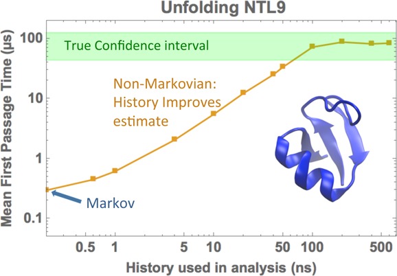
Because standard molecular dynamics (MD) simulations are unable to access time scales of interest in complex biomolecular systems, it is common to “stitch together” information from multiple shorter trajectories using approximate Markov state model (MSM) analysis. However, MSMs may require significant tuning and can yield biased results. Here, by analyzing some of the longest protein MD data sets available (>100 μs per protein), we show that estimators constructed based on exact non-Markovian (NM) principles can yield significantly improved mean first-passage times (MFPTs) for protein folding and unfolding. In some cases, MSM bias of more than an order of magnitude can be corrected when identical trajectory data are reanalyzed by non-Markovian approaches. The NM analysis includes “history” information, higher order time correlations compared to MSMs, that is available in every MD trajectory. The NM strategy is insensitive to fine details of the states used and works well when a fine time-discretization (i.e., small “lag time”) is used.

1. Introduction

The field of biomolecular simulation is poised at a moment of opportunity and challenge: with current parallel and distributed computing capabilities, vast amounts of trajectory data can readily be generated; however, the optimal means of orchestrating simulations and analyzing the output remain unresolved. Currently, a number of sophisticated approaches, such as “replica exchange”,¹⁻⁴ path-sampling,⁵⁻⁹ and other strategies,¹⁰⁻¹³ provide precise prescriptions for the generation and analysis of trajectories. In another popular approach, large collections of relatively short molecular dynamics (MD) trajectories initiated in diverse regions of configuration space are often analyzed using Markov state models (MSMs) which assume that future dynamics depends only on the present state and not on prior history.¹⁴⁻¹⁶ Extremely long continuous MD trajectories have also been generated and subjected to an array of analyses.¹⁷⁻²⁰

The present report attempts to improve on the analysis of MD data, which in turn can aid in optimizing the design of increasingly common multiple-trajectory studies.²¹ By improving the extraction of kinetic information from trajectory segments, which can depend on segment length, this work offers quantitative insight into optimizing the allocation of resources. The focus of the present study is estimation of the slowest “macroscopic” time scales, particularly the mean first-passage time (MFPT) for protein folding and unfolding events. The MFPT is a standard definition of the inverse rate for a process.²² All of the analyses discussed are general and also apply to rate estimation for conformational change and (un)binding processes.

Our work builds on the extensive theory and software development that already underpins MSMs.^{14−16,21,23−25} MSM estimation of kinetic behavior typically proceeds from a particular set of trajectory data by (i) subdivision of the full configuration space into distinct regions or “states” based on clustering of trajectory configurations, (ii) generating a history-independent transition matrix based on transition counts observed in the data, (iii) extracting “implied time scales” based on dominant eigenvalues, often as a function of lag time (time-discretization), and (iv) repeating the process multiple times because of the nonuniqueness of clustering to ensure robust estimation of time scales. Our revised procedure modifies steps (ii) and (iii) to account for history information. We also revisit the issues of lag-time dependence and sensitivity to clustering in MSMs. We note that, in contrast to (i), alternative procedures for constructing states that do not include all of the configuration space have been proposed for Markov analysis,²⁶⁻²⁸ but those procedures are not generally used for trajectory postanalysis and will not be considered here.

It is essential to recognize that even when the underlying dynamics of a continuous system (e.g., molecular) is Markovian, the system’s behavior becomes non-Markovian when projected onto a finite discrete space.²⁹ A simple example illustrates the point. Consider a particle exhibiting simple diffusive continuous dynamics in a one-dimensional space: when the space is divided into finite sequentially numbered states, the probability to transition from state i to i+1 will depend on whether the particle entered state i from i–1 (further away from i+1) or from i+1 (closer). The issue becomes more pronounced when projecting from a high-dimensional space to a relatively small number of discrete states.

A key non-Markovian precedent for this work is the unbiased procedure for calculating the MFPT when sufficient history information is present in the trajectory data set.³⁰⁻³³ Specifically, the MFPT for a transition between arbitrary “macrostates” A and B can be estimated without bias from a transition matrix calculated using “last-in-A” trajectories, i.e., the subset of trajectories which can be traced back in time and were more recently in state A than B. Remarkably, this result holds regardless of the clustering or division of configuration space defining the transition matrix.³² However, MFPT estimates generally will be biased when trajectories do not satisfy the last-in-A requirement.³²

An important distinction of the present approach is the focus on well-defined time scales between specified states, in contrast to calculating less specific “implied time scales”. The choice is motivated by the interest of many investigators in specific processes (e.g., folding, functional conformational changes), and equally importantly, the ability to compare MFPT estimates with independent reference calculations. In particular, recent μs–ms scale MD simulations exhibiting multiple protein folding and unfolding events¹⁷ provide an unprecedented opportunity for quantitative validation of the approach.

We construct and test a series of non-Markovian (NM) MFPT estimators, i.e., estimators that use trajectory history in constructing transition matrices. The most useful estimators are guaranteed to recover unbiased MFPT values, for the lag-time used, when trajectories possess sufficient history information, independently of the partition of the space into states. The data show that using configuration-space clustering generated by standard MSM software, the NM estimators provide MFPT values in substantially better agreement with long-trajectory reference values, compared to MSM estimates, for every system and every trajectory set examined. The NM estimators function equally well with crude states based on a simple coordinate.

2. Theoretical Formulation

2.1. MFPT, Lag Time, and Discretization Error

The MFPT is the primary kinetic observable studied in this report because its inverse quantifies the rate of a process such as folding. The MFPT is the mean time to first reach a defined target state “B” (e.g., the folded state of a protein) starting from a defined initial distribution in state “A” (e.g., the unfolded state).

To estimate the MFPT accurately, it is essential to understand its relation to the lag time τ, the fixed interval at which trajectory data is examined. Kinetic observables fundamentally are defined by the τ → 0 limit, although considerations of expediency may motivate use of larger τ: for example, in the molecular simulation trajectories analyzed below, configurations have been saved only every δt = 0.2 ns. Whenever τ is finite, discretization error must be expected, but the error in the MFPT should be negligible for the small τ = δt = 0.2 ns used in the present analysis. Importantly, τ is not an upper bound on the discretization error in the MFPT because of potential recrossing of the state B boundary, which can be a significant effect.

Regardless of how the target state of a first-passage process is defined, one expects discretization error in the MFPT to increase monotonically with τ because eliminating trajectory points can only delay arrival to the target state. This behavior is indeed seen for protein folding and unfolding (see Figures S1–S6 in Supporting Information (SI)).

Importantly, the long lag-time limit of the MFPT does not depend on the kinetics of a system but instead is completely specified by the equilibrium probability of the target state p^eq(B) via MFPT(τ → ∞) ∼ τ/p^eq(B). Increasing the lag time in any MFPT analysis (Markov or otherwise) thus presents the danger of introducing artifactual (nonkinetic) dependence. For these reasons, this report considers only τ = δt.

2.2. Markovian Estimation of the MFPT

The main focus of this report is the non-Markovian estimation of observables, but for reference, we also perform traditional Markov analysis of the trajectories. In a MSM, the full configuration space is first divided into relatively small states, and kinetic analysis is performed without employing history information.^{14−16,21,23−25} That is, the rate k_ij between states i and j is defined as the conditional transition probability

1

where X_t is the random variable representing the state of the system at time t, and τ is the lag-time used for the Markov model. Each rate can be estimated by the maximum likelihood estimator (MLE) c_ij/∑_jc_ij,²⁴ where c_ij are elements of the count matrix C, the total number of i-to-j transitions observed during the simulation at the given lag-time.

However, since we we will be analyzing equilibrium ensembles where detailed balance must hold, it is more convenient to introduce that symmetry directly to our Markov model. Algorithms to compute the MLE of the transition matrix for reversible Markov models are well-known,^23,24,34 and here, we follow the one proposed by Prinz et al.²⁴ The MFPT is then computed analytically following ref (32).

Importantly, MSM MFPT estimates generally are biased, as the data below shows. This is true even when the MSM is built from a single continuous trajectory many times the length of the MFPT. As noted, discrete state dynamics are intrinsically non-Markovian, so bias in MFPT estimation should be expected.

2.3. Non-Markovian Calculation of the MFPT without Bias Using Full History

Although our primary focus is the analysis of limited-history trajectory segments (with segment length less than the MFPT), we develop estimators based on exact procedures available when complete history information is available. We now briefly describe the full-history procedures, which are detailed elsewhere.³⁰⁻³³

To calculate a MFPT, the exact procedure requires only a single history-based label indicating whether macroscopic state A or B was visited most recently. Trajectories most recently (or currently) in A are given the α label, and β denotes those most recently in B. See Figure 1a. Such labels may be called “color” information. States A and B cannot be overlapping, but their union need not cover the full phase space. For convenience, we take A and B to consist precisely of subsets of nonmacroscopic states i.

Figure 1.

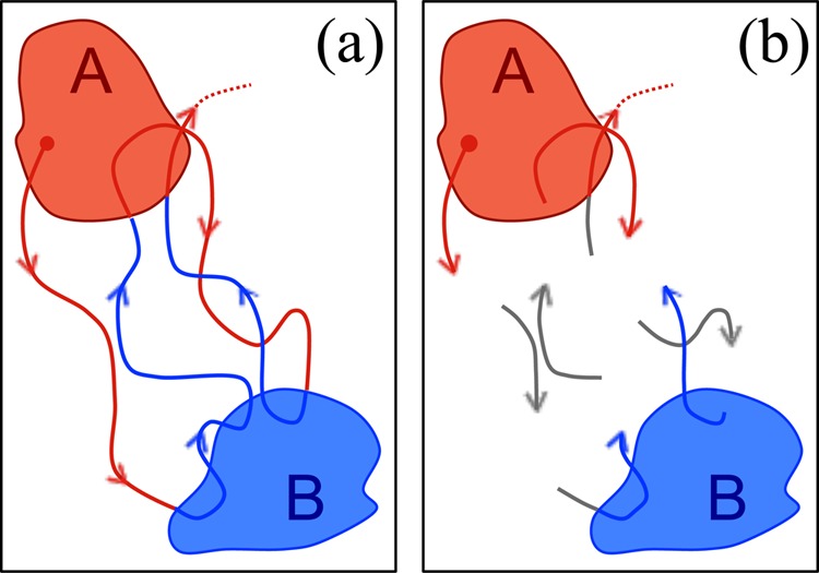
Non-Markovian trajectory analysis with full and partial data. (a) Schematic representation of a single continuous trajectory where the color indicates the last state visited: blue trajectories were last in state B and red trajectories were last in A. (b) Multiple trajectory segments where color information is not always known, as indicated by gray and partially gray segments.

If one considers a large equilibrium ensemble of labeled trajectories, each nonmacroscopic state i will contain both α and β trajectories that must together sum to the equilibrium probability

2

With N states, a set of 2N probabilities is therefore required.

Similarly, a 2N × 2N “colored” rate matrix is used for MFPT estimation, where there are now two additional history labels μ and ν (either α or β) for each element of the transition matrix {k_ij^μν} that track whether the label has changed.^29,32 Only if a trajectory enters a new macrostate will ν change from μ.

Formally, we have

3

where L_t and L_t+τ account for the label of the trajectory (α or β) before and after the lag time τ, respectively.

Solving the steady-state solution of the matrix with elements {k_ij^μν} yields both equilibrium and unbiased kinetic information, as described previously.^29,32 The steady state essentially describes the circulating flow of trajectories as they continually make transitions and switch back and forth between α and β labels. Equilibrium information is obtained simply by summing labeled probabilities via (2), whereas unbiased MFPT estimates result from computing fluxes solely based on a specific label α or β.^29,32 In contrast, MSM-based MFPT estimates fail to separate the α and β components, leading to bias.

2.4. Second-Order Markov Models for Using Additional History

Given the value of history information in generating unbiased MFPT estimates, we consider a number of alternatives for using information beyond the two time-point pairs employed by typical MSMs. We first examine second-order Markov analyses, as sketched in Figure 2.

Figure 2.

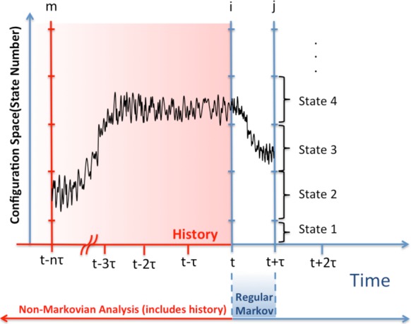
Schematic representation of the second-order Markov analysis. The y-axis represents the continuous configuration space divided in discrete states (shown at right). Regular Markov analysis examines two time points, t and t + τ, whereas the second-order analysis additionally considers the system state at time t – nτ for arbitrary n, which is a form of history information.

The rates in a second-order Markov model have three indexes since they will depend on states the system visited at two prior time points. For maximum generality, we consider the family of such models where the prior time points are separated by an arbitrary multiple n of the lag time; rates are defined by

4

where n can be adjusted for the given τ (see Figure 2). If n = 0, the rates and results are equivalent to a regular first order Markov model. The same is true when n → ∞ since the transition between i and j becomes independent of what happened in the very distant past.

As described in the SI, numerical estimates of the MFPT are obtained by kinetic simulation using the transition probabilities specified in the rate matrix at every time step.

2.5. Non-Markovian Estimation of the MFPT with Limited “Color” Information

Building further on the sufficiency of the “color” labels α and β for the unbiased MFPT calculation described above, we now construct approximate estimators applicable to sets of trajectories that may lack color labels in some instances (see Figure 1b). A finite trajectory segment will lack a label, for example, if it never visits either initial macrostate A or target state B. The new estimators use color information if it is available and otherwise assign labels based on Markovian statistical models.

More precisely, the construction of the rate matrix used for MFPT estimation proceeds in two steps. First, elements of the 2N × 2N colored rate matrix are assigned preliminary label-independent values, k_ij^μν = k_ij based on all trajectory data, which provides estimates for p_i and p_i^β in a Markovian picture. Second, the colored matrix is completely recalculated by examining each pair of τ-separated points in every trajectory. If a given segment possesses sufficient history to assign an α or β label, that is done. If not, the label μ is assigned with probability p_i/p_i^eq previously inferred from the preliminary Markov calculation. This procedure is used to construct the approximate colored 2N × 2N count matrix C = {c_ij}, that is transformed into the rate matrix used for MFPT estimation by the same steady-state procedure noted above. This procedure defines the “Markov+Color” estimator used throughout the study.

We can define a similar MFPT estimator combining color information with the second-order Markov models described above. As for the “Markov+Color” estimator, we use the color information when it is available, but the procedure is somewhat different because the MFPT ultimately will be determined via kinetic simulation. We examine each trajectory segment using a fixed n value and determine whether either macroscopic state A or B was visited between t–nτ and t. If neither was visited during this interval, the state m is used as the third element of the three-dimensional (3D) matrix in eq 4. Otherwise, the “color” index (α or β) is stored instead. In practice, for limited history windows corresponding to small n values, color information will rarely be available.

A numerical estimate of the MFPT, termed “2nd-Markov+Color” is obtained by kinetic simulation based on the 3D rate matrix.

By construction, both partial-history estimators, Markov+ Color and second-order Markov+Color, converge to the true MFPT when sufficiently long trajectories are available. Below, we show the dependence of all the estimators as a function of the history length, defined as the maximum time length we are allow to go back in time in order to assign a color label or a previous system state (see SI for further details).

2.6. History Length

Although we have very long trajectories available, we want to mimic the effects of having shorter fragments. We define the (nominal) history length as the maximum time we review in order to assign color labels or a previous system state. However, the effective or average history length actually used will depend on the length of the trajectory fragments we are considering. If the fragments are very long as compared to the history length we are considering, then the nominal history length and the effective history length used are going to be very similar.

To understand this, consider, for instance, that our fragments have n+1 time points, and we want to analyze them with a history length n. That history length can only be used completely in the last point of the fragment, and in general, for the time point k we can only go back in history k–1 steps, even when the history length we are considering is n > k. In average, in this case, the effective history length used would be (n+1)/2.

3. Systems, Model Construction, and Reference Values

3.1. Model Systems and Macrostate Definitions

We analyzed trajectories for four proteins previously studied in explicit solvent by μs–ms scale atomistic molecular dynamics simulations generated using the special purpose Anton supercomputer.¹⁷ We examined Chignolin, Trp-cage, NTL9, and Villin. In the case of NTL9, more than one trajectory was available, but we only analyzed the longest trajectory reported.

Table 1 shows, for each system, the RMSD basis of the folded and unfolded macrostates, the Protein Data Bank code of the reference structure used for RMSD calculation, the total simulation time considered for the analysis and the number of residues. Further details about the trajectories can be found in the original paper.¹⁷

Table 1. Protein Models Used for Markovian and Non-Markovian Analyses^a.

protein	num. residues	time (μs)	RMSD (folded)	RMSD (unfolded)	reference structure (PDB ID)
chignolin	10	106	<1.10 Å	>7.0 Å	5AWL
Trp-cage	20	208	<1.75 Å	>10.0 Å	2JOF
NTL9	39	1100	<1.50 Å	>10.0 Å	2HBA
villin	35	125	<1.50 Å	>11.0 Å	2F4K

^aFor each system, the table shows the number of residues, the total simulation time used in the analysis, and the state definitions based on heavy-atom RMSD with respect to the folded structure whose protein data bank code (PDB ID) is given in the last column.

3.2. Markov State Model Construction with “Optimized” Bins

Trajectories were projected into a reduced dimension space represented by the ϕ, ψ, and χ₁ dihedral angles of each residue of the protein. Each frame of the trajectory was then characterized by a vector containing the sine and cosine of each of these torsions in order to account for the periodicity of the angles. We applied time-independent component analysis (tICA) to further reduce the dimensionality of the model space before constructing the Markov state model.^35,36 All transformations of the trajectory data, along with subsequent construction of the MSM were performed using MSMBuilder3³⁴ together with MDTraj.³⁷

We then constructed a large set of candidate MSMs by varying the hyperparameters of the model, specifically the number of microstates (clusters), tICA components and both the lag time of the MSM and the lag time used in determining the tICA components. The grid of tested parameters is shown in Table 2, and iterating over all combinations of parameters resulted in 576 distinct models.

Table 2. MSM Hyperparameters.

hyperparameter	grid search values
number of tICA components	1, 2, 4, 8
tICA lag time (ns)	50, 100, 200
number of MSM microstates	50, 100, 250, 500, 1000,
	2000, 4000, 8000
MSM lag time (ns)	0.2, 5, 10, 25, 50, 100

A subset of these models was then selected for further analysis based on the MFPTs of folding and unfolding calculated from projecting the full continuous trajectory onto the space of discrete states. If the dynamics in the discrete space reproduced the MFPTs calculated from the continuous trajectories¹⁷ to within a reasonable interval (see Table 3), then the model is considered as acceptable and used in subsequent analysis. Here, we refer not to MSM behavior, but merely the averaging of first-passage events occurring in the long continuous trajectories when mapped on to the discrete-state model with macrostates defined in the manner described above. Models not reproducing established MFPTs were discarded to avoid artifactual MFPT behavior in both MSM and non-Markov analysis.

Table 3. Definitions of Acceptable Models^a.

	MFPT interval (μs)
protein	folding	unfolding
chignolin	0.1–3.0	0.5–8.0
Trp-cage	8.0–10	1.0–5.0
NTL9	5.0–30	75–250
villin	1.0–5.0	0.2–3.0

^aThe models with MFPTs within the intervals shown around the values reported in the literature¹⁷ are considered as good models and otherwise are discarded.

Definitions of the folded and unfolded states in the discrete space were defined by examining the mean RMSD to the native conformation of all frames assigned to a particular cluster subject to a system-specific cutoff (see Table 1). That is, if the average RMSD within a cluster was within the specified RMSD cutoff, the cluster/state was considered part of the corresponding macrostate, folded or unfolded. Definitions of the unfolded and folded states for the continuous trajectories were also defined using a dual-cutoff approach as in ref (38).

Culling models with state-spaces that are unable to reproduce MFPTs generated from the full continuous trajectories ensures that a reasonable comparison can be made between different estimators and the long brute-force trajectories.

3.3. RMSD-Based States

In addition to the partition of the systems in states as previously described using the tools given by MSMBuilder3³⁴ and for the sake of comparison, we also examined the results from a simple RMSD partition, with respect to the folded structure, of the space where the folded and unfolded states are defined by single states, and the intermediate region is evenly divided in 48 additional states. The definition of folded and unfolded states in terms of the RMSD are given in Table 1.

3.4. Reference Calculation of Observables from Long Trajectories

All the simulations analyzed here are single regular molecular dynamics trajectories¹⁷ that were saved every 0.2 ns. The first passage times we use as reference are measured and averaged at that time resolution directly during the simulations by tracing the evolution of the trajectories and recording the time points at which the trajectories entered and exited the folded and unfolded states. Folded and unfolded state definitions are given above.

4. Results and Discussion

We compare non-Markov and Markov estimates of the MFPT using trajectory data previously generated¹⁷ for four peptides and proteins: Chignolin, Trp-cage, the Villin headpiece, and NTL9 (see Figure 3). The available trajectory data contain at least 10 events of each type for every system, providing reliable reference values. The analyses are performed on models using two approaches to dividing configuration space: (i) states constructed by the MSMBuilder software (v3.3)³⁴ and (ii) simple states based on subdividing a single coordinate, the RMSD with respect to the folded structure. Further, we perform analyses using all the available data, as well as subsets corresponding to less than the sum of folding and unfolding MFPTs.

Figure 3.

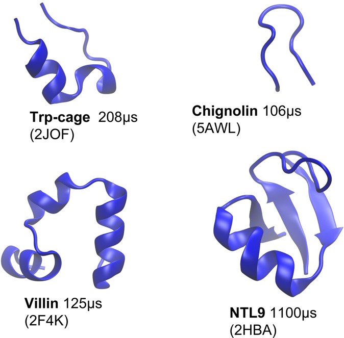
Four proteins studied. The total simulation time is shown along with the Protein Data Bank entry of the experimental structure.

After analyzing hundreds of models for each protein with reasonable agreement with the MFPTs reported,¹⁷ we found that the dependence of the estimated Markovian MFPTs on the number of states is very small as compared to the strong sensitivity to the lag-time. For that reason, we decided to choose a model for further analyses, for each protein, with only 50 states. The model was selected randomly among all the acceptable models we generated.

Non-Markovian MFPT estimates are shown along with Markov-based values for reference. For the model selected in each system, the lag time used is τ = 0.2ns, which is the time interval used to store trajectory snapshots and hence minimizes the discretization error discussed above. (Figures S1–S6 motivate our choice, showing there is considerable ambiguity and potential error in selecting a longer lag time.) As the data show, the bias in the MFPTs can be corrected by just considering a relatively limited amount of history in the analysis.

4.1. MFPT Estimates Using All Data

4.1.1. MSM-Optimized States

We performed different analyses on states constructed via MSMBuilder.

First, we confirmed the correctness of the non-Markovian analysis previously proposed^29,32 and described by eq 3. We generated MFPT estimates from the steady-state solution of the rate matrix (3), with matrix elements calculated based on the full trajectories. Thus, we used all available history information, and every segment could be categorized according to a label α or β. These matrix-based MFPT estimates were compared with reference values obtained by direct averaging of FPTs obtained from the long trajectories. Figure 4 shows the excellent agreement for all the proteins’ folding and unfolding times and motivates pursuing history-based MFPT estimation using less history.

Figure 4.

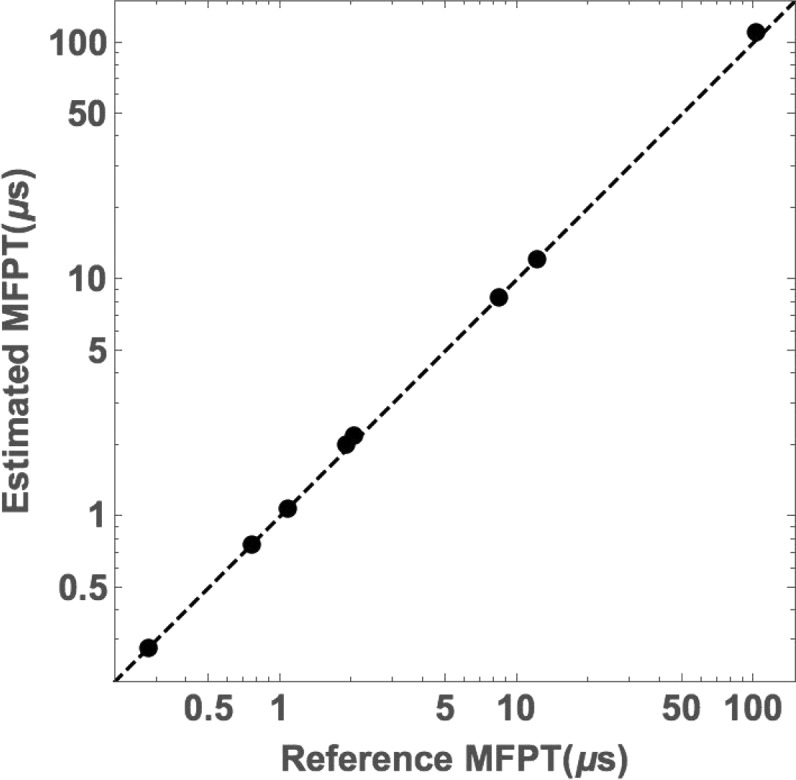
Exactness of the “color”-labeled formulation. Comparison of reference MFPT values for both folding and unfolding of all four proteins with MFPT estimates from solving the steady-state solution of the labeled rate matrix (eq 3) when the full continuous trajectories are used to assign color labels, i.e., when all available history information is used. Reference values are direct averages of first-passage times from the trajectories.

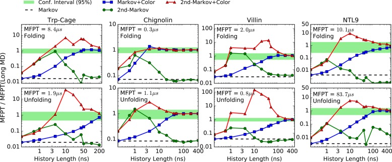
We next examined the effects of reducing the amount of history information used in MFPT estimation, as shown in Figure 5. Although all trajectory data are included, the non-Markovian estimates use only the finite amount of history indicated on the horizontal axis. Both estimators using color labels (when available) can drastically reduce the bias based on a history length significantly shorter than the MFPTs themselves. The amount of history needed is of the order of the transition event duration, t_b,³⁹ which is usually very small as compared to the MFPTs.

Figure 5.

MFPT estimates for protein folding (first row) and unfolding (second row) using MSM-optimized states. MFPT values are normalized by reference values (shown with text) obtained from long MD simulations¹⁷ at the shortest lag time. The plots show the dependence of the various estimators on the history length used (see text). The green horizontal stripes are the 95% confidence interval for the reference values.

In general, the second-order Markov approach improves the estimate for short history lengths but then converges to the Markovian value as expected. Only if color history information is included do first-order and second-order Markov estimates converge to the exact value. In every case, the (history independent) Markov MFPT estimates are significantly shorter than the reference value, by one or more orders of magnitude. Although Markov MFPT estimates based on longer lag times do increase, their large-τ behavior is linear and ultimately must exceed the reference value; as shown in the SI, there is no unambiguous way to select a longer lag time and longer lags certainly include discretization error.

4.2. Simple RMSD-Based States

Because construction of a MSM is not a simple task that may require some degree of user curation, we also examined MFPT estimates based on very simple coordinates. We chose RMSD from the (experimental) folded state because it is straightforward to calculate and interpret, although it has well-known weaknesses.⁴⁰

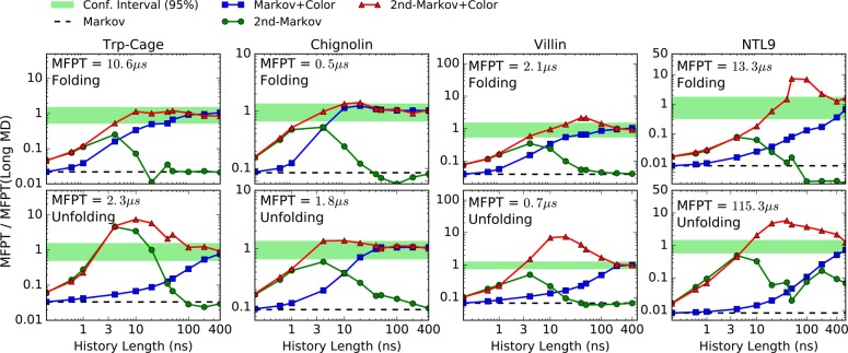
With enough history information, the “quality” of the states does not seem to negatively affect our non-Markovian estimators. If simple states based on subdividing the RMSD with respect to the folded structure (see SI for further details) are used, we still have unbiased results when the color information is considered (Figure 6). Because the states used for the RMSD-based analysis differ slightly from those based on MSM-optimized states, the absolute MFPT values differ slightly as well.

Figure 6.

MFPT estimates for protein folding (first row) and unfolding (second row) using RMSD-based states. MFPT values are normalized by reference values (shown with text) obtained from long MD simulations¹⁷ at the shortest lag time. The plots show the dependence of the various estimators on the history length used (see text). The green horizontal stripes are the 95% confidence interval for the reference values. Note that absolute MFPT values differ slightly from those in Figure 5; see text.

4.3. Estimates with Reduced data and MSM-Optimized States

A major goal of trajectory analysis is to predict the long time behavior of a system using a minimum amount of data, i.e., a subset that can be generated affordably. Because the preceding results show that the amount of history needed to obtain satisfactory results is small compared to the MFPTs, and in general as compared to the longest time scales of the system, it is reasonable to think that multiple short trajectories starting from different regions of the configurational space would be a valid way to predict observables.

We mimic low-data scenarios by dividing the continuous trajectories of Chignolin, Trp-Cage, and Villin in fragments of 0.5 μs and the trajectory of NTL9 in fragments of 1.0 μs, again using states constructed by MSMBuilder. Such trajectory sets can be considered an idealized use case without artifacts from initiating multiple trajectories and hence constitute at least a minimal test for any valid analysis. In all cases, the length of the MFPT is significantly longer than the fragment size (see Figure 5). MFPTs are estimated from a small fraction of the fragments, chosen with replacement and limiting the number of trajectories starting in each state.

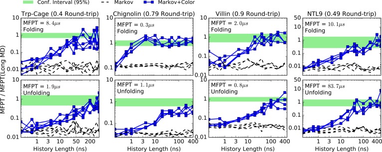
When the amount of trajectory data is drastically reduced, the second-order approaches start to fail because there are more parameters to estimate with the same amount of information. Here, we will only show results when the data are reduced bellow 5% of the original data, as this is the regime of greatest practical interest. Because the second-order approaches are overwhelmed by noise in the low-data regime, we only show first-order estimates employing color information.

Figure 7 shows that the Markov+Color estimator functions well in the low-data regimes when the history length is sufficient. Most of the bias is removed, as compared with the history-independent Markov estimator. The fluctuations in Markov estimates are not true history dependence but simply noise since every point in the plots is generated from an independent subsample, extracted with replacement from the full data set.

Figure 7.

Folding (first row) and unfolding (second row) MFPT estimates using MSM-optimized states. The estimations were done from subsamples that represent less than 5% of the available MD data¹⁷ for each protein at the shortest lag time. For each value of history length, four independent subsamples were extracted with replacement. A pair of folding and unfolding MFPT curves is generated using a total amount of trajectory data less than the round-trip time (sum of forward and backward MFPTs), as indicated for each protein.

4.4. Estimates with Reduced Data, Simple RMSD-Based States

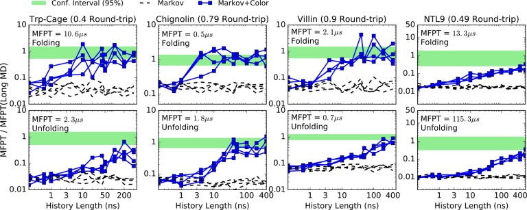
Figure 8 shows MFPTs estimated from a small fraction of the simulation extracted as described in the previous section. In this case, the model was built from simple RMSD-based bins.

Figure 8.

Folding (first row) and unfolding (second row) MFPT estimates using RMSD-based states. The estimations were done from subsamples that represent less than 5% of the available MD data¹⁷ for each protein at the shortest lag time. For each value of history length, four independent subsamples were extracted with replacement. A pair of folding and unfolding MFPT curves is generated using a total amount of trajectory data less than the round-trip time (sum of forward and backward MFPTs), as indicated for each protein.

5. Conclusions and Outlook

When projected onto finite discrete spaces, molecular dynamics is intrinsically non-Markovian, i.e., it is history-dependent. By analyzing continuous trajectories that exhibit multiple (un)folding transitions and reliable MFPT values, our data indicate that non-Markovian analyses offer the prospect of drastically reducing the bias intrinsic to history-independent Markov MFPT estimation. For the proteins considered here, this conclusion holds regardless of whether configuration space was subdivided using sophisticated approaches with MSM-optimized states or much simpler “bins” in a one-dimensional RMSD space. Importantly, the non-Markov analyses are readily applied at the shortest lag times where the discretization error is minimal. We note that the bias in MSMs reported here has been observed in the context of standard MSMs used for postanalysis which tile configuration space so that the union of the states or clusters comprises the full configuration space.

Although the non-Markovian estimators offer clear advantages, their optimal use in typical cases may require somewhat longer trajectory segments (hundreds of nanoseconds or more) than were readily available in the past; however, given modern computing hardware, such trajectory sets may soon be routinely available. Further, because the non-Markovian estimators converge to the unbiased MFPT, their behavior with varying history length offers a self-diagnostic tool. The main conclusion, in any case, is that analysis of complex systems should exploit history information when it is available. Future work will explore the effects of non-Markovian analysis on pathway inference.

Glossary

Abbreviations

MSM

Markov state model

NM

non-Markovian

RMSD

root mean-squared deviation

Supporting Information Available

The Supporting Information is available free of charge on the ACS Publications website at DOI: 10.1021/acs.jctc.6b00339.

• Data describing the MFPT dependence on τ and the number of states are shown as well as descriptions of software and algorithms to calculate MFPTs (PDF)

This work was partially supported by NIH Grants R01GM115805 and P41GM103712, as well as NSF Grant MCB-1119091.

The authors declare no competing financial interest.

References

- Hukushima K.; Nemoto K. J. Phys. Soc. Jpn. 1996, 65, 1604–1608. 10.1143/JPSJ.65.1604. [DOI] [Google Scholar]
- Meng Y.; Roitberg A. E. J. Chem. Theory Comput. 2010, 6, 1401–1412. 10.1021/ct900676b. [DOI] [PMC free article] [PubMed] [Google Scholar]
- Nadler W.; Hansmann U. H. E. Phys. Rev. E Stat. Nonlin. Soft Matter Phys. 2007, 76, 065701. 10.1103/PhysRevE.76.065701. [DOI] [PubMed] [Google Scholar]
- Okumura H.; Gallicchio E.; Levy R. M. J. Comput. Chem. 2010, 31, 1357–1367. 10.1002/jcc.21419. [DOI] [PMC free article] [PubMed] [Google Scholar]
- Allen R. J.; Warren P. B.; ten Wolde P. R. Phys. Rev. Lett. 2005, 94, 018104. 10.1103/PhysRevLett.94.018104. [DOI] [PubMed] [Google Scholar]
- van Erp T. S.; Moroni D.; Bolhuis P. G. J. Chem. Phys. 2003, 118, 7762–7774. 10.1063/1.1562614. [DOI] [Google Scholar]
- Moroni D.; Bolhuis P. G.; van Erp T. S. J. Chem. Phys. 2004, 120, 4055–4065. 10.1063/1.1644537. [DOI] [PubMed] [Google Scholar]
- Moroni D.; van Erp T. S.; Bolhuis P. G. Phys. Rev. E Stat. Nonlin. Soft Matter Phys. 2005, 71, 056709. 10.1103/PhysRevE.71.056709. [DOI] [PubMed] [Google Scholar]
- Valeriani C.; Allen R. J.; Morelli M. J.; Frenkel D.; ten Wolde P. R. J. Chem. Phys. 2007, 127, 114109. 10.1063/1.2767625. [DOI] [PubMed] [Google Scholar]
- Laio A.; Parrinello M. Proc. Natl. Acad. Sci. U. S. A. 2002, 99, 12562–12566. 10.1073/pnas.202427399. [DOI] [PMC free article] [PubMed] [Google Scholar]
- Bussi G.; Laio A.; Parrinello M. Phys. Rev. Lett. 2006, 96, 090601. 10.1103/PhysRevLett.96.090601. [DOI] [PubMed] [Google Scholar]
- Vargiu A. V.; Ruggerone P.; Magistrato A.; Carloni P. Nucleic Acids Res. 2008, 36, 5910–5921. 10.1093/nar/gkn561. [DOI] [PMC free article] [PubMed] [Google Scholar]
- Tiwary P.; Parrinello M. Phys. Rev. Lett. 2013, 111, 230602. 10.1103/PhysRevLett.111.230602. [DOI] [PubMed] [Google Scholar]
- Noé F.; Horenko I.; Schütte C.; Smith J. C. J. Chem. Phys. 2007, 126, 155102. 10.1063/1.2714539. [DOI] [PubMed] [Google Scholar]
- Chodera J. D.; Singhal N.; Pande V. S.; Dill K. A.; Swope W. C. J. Chem. Phys. 2007, 126, 155101–17. 10.1063/1.2714538. [DOI] [PubMed] [Google Scholar]
- Bowman G. R.; Ensign D. L.; Pande V. S. J. Chem. Theory Comput. 2010, 6, 787–794. 10.1021/ct900620b. [DOI] [PMC free article] [PubMed] [Google Scholar]
- Lindorff-Larsen K.; Piana S.; Dror R. O.; Shaw D. E. Science 2011, 334, 517–520. 10.1126/science.1208351. [DOI] [PubMed] [Google Scholar]
- Schwantes C. R.; Pande V. S. J. Chem. Theory Comput. 2013, 9, 2000–2009. 10.1021/ct300878a. [DOI] [PMC free article] [PubMed] [Google Scholar]
- Malmstrom R. D.; Lee C. T.; Wart A. T. V.; Amaro R. E. J. Chem. Theory Comput. 2014, 10, 2648–2657. 10.1021/ct5002363. [DOI] [PMC free article] [PubMed] [Google Scholar]
- Deng N.; Dai W.; Levy R. M. J. Phys. Chem. B 2013, 117, 12787–12799. 10.1021/jp401962k. [DOI] [PMC free article] [PubMed] [Google Scholar]
- Noé F.; Schütte C.; Vanden-Eijnden E.; Reich L.; Weikl T. R. Proc. Natl. Acad. Sci. U. S. A. 2009, 106, 19011–19016. 10.1073/pnas.0905466106. [DOI] [PMC free article] [PubMed] [Google Scholar]
- Reimann P.; Schmid G. J.; Hanggi P. Phys. Rev. E: Stat. Phys., Plasmas, Fluids, Relat. Interdiscip. Top. 1999, 60, R1. 10.1103/PhysRevE.60.R1. [DOI] [PubMed] [Google Scholar]
- Bowman G. R.; Beauchamp K. A.; Boxer G.; Pande V. S. J. Chem. Phys. 2009, 131, 124101. 10.1063/1.3216567. [DOI] [PMC free article] [PubMed] [Google Scholar]
- Prinz J.-H.; Wu H.; Sarich M.; Keller B.; Senne M.; Held M.; Chodera J. D.; Schütte C.; Noé F. J. Chem. Phys. 2011, 134, 174105. 10.1063/1.3565032. [DOI] [PubMed] [Google Scholar]
- Bowman G. R.; Pande V. S.; Noé F.. An Introduction to Markov State Models and Their Application to Long Timescale Molecular Simulation; Springer: Dordrecht, The Netherlands, 2014. [Google Scholar]
- Schütte C.; Noé F.; Lu J.; Sarich M.; Vanden-Eijnden E. J. Chem. Phys. 2011, 134, 204105. 10.1063/1.3590108. [DOI] [PubMed] [Google Scholar]
- Faradjian A. K.; Elber R. J. Chem. Phys. 2004, 120, 10880–10889. 10.1063/1.1738640. [DOI] [PubMed] [Google Scholar]
- Bello-Rivas J. M.; Elber R. J. Chem. Phys. 2015, 142, 094102. 10.1063/1.4913399. [DOI] [PMC free article] [PubMed] [Google Scholar]
- Suárez E.; Pratt A. J.; Chong L. T.; Zuckerman D. M. Protein Sci. 2016, 25, 67–78. 10.1002/pro.2738. [DOI] [PMC free article] [PubMed] [Google Scholar]
- Vanden-Eijnden E.; Venturoli M. J. Chem. Phys. 2009, 131, 044120. 10.1063/1.3180821. [DOI] [PubMed] [Google Scholar]
- Dickson A.; Warmflash A.; Dinner A. R. J. Chem. Phys. 2009, 131, 154104. 10.1063/1.3244561. [DOI] [PubMed] [Google Scholar]
- Suárez E.; Lettieri S.; Zwier M. C.; Stringer C. A.; Raman Subramanian S.; Chong L. T.; Zuckerman D. M. J. Chem. Theory Comput. 2014, 10, 2658–2667. 10.1021/ct401065r. [DOI] [PMC free article] [PubMed] [Google Scholar]
- Adelman J. L.; Grabe M. J. Chem. Theory Comput. 2015, 11, 1907–1918. 10.1021/ct501134s. [DOI] [PMC free article] [PubMed] [Google Scholar]
- Beauchamp K. A.; Bowman G. R.; Lane T. J.; Maibaum L.; Haque I. S.; Pande V. S. J. Chem. Theory Comput. 2011, 7, 3412–3419. 10.1021/ct200463m. [DOI] [PMC free article] [PubMed] [Google Scholar]
- Pérez-Hernández G.; Paul F.; Giorgino T.; De Fabritiis G.; Noé F. J. Chem. Phys. 2013, 139, 015102. 10.1063/1.4811489. [DOI] [PubMed] [Google Scholar]
- McGibbon R.; Beauchamp K.; Harrigan M.; Klein C.; Swails J.; Hernández C.; Schwantes C.; Wang L.-P.; Lane T.; Pande V. Biophys. J. 2015, 109, 1528–1532. 10.1016/j.bpj.2015.08.015. [DOI] [PMC free article] [PubMed] [Google Scholar]
- Piana S.; Lindorff-Larsen K.; Shaw D. E. Biophys. J. 2011, 100, L47–9. 10.1016/j.bpj.2011.03.051. [DOI] [PMC free article] [PubMed] [Google Scholar]
- Zuckerman D. M.; Woolf T. B. J. Chem. Phys. 2002, 116, 2586–2591. 10.1063/1.1433501. [DOI] [Google Scholar]
- Zhang B. W.; Jasnow D.; Zuckerman D. M. Proc. Natl. Acad. Sci. U. S. A. 2007, 104, 18043–18048. 10.1073/pnas.0706349104. [DOI] [PMC free article] [PubMed] [Google Scholar]
Associated Data
This section collects any data citations, data availability statements, or supplementary materials included in this article.