

ABSTRACT
Detailed anatomical understanding of the human brain is essential for unraveling its functional architecture, yet current reference atlases have major limitations such as lack of whole‐brain coverage, relatively low image resolution, and sparse structural annotation. We present the first digital human brain atlas to incorporate neuroimaging, high‐resolution histology, and chemoarchitecture across a complete adult female brain, consisting of magnetic resonance imaging (MRI), diffusion‐weighted imaging (DWI), and 1,356 large‐format cellular resolution (1 µm/pixel) Nissl and immunohistochemistry anatomical plates. The atlas is comprehensively annotated for 862 structures, including 117 white matter tracts and several novel cyto‐ and chemoarchitecturally defined structures, and these annotations were transferred onto the matching MRI dataset. Neocortical delineations were done for sulci, gyri, and modified Brodmann areas to link macroscopic anatomical and microscopic cytoarchitectural parcellations. Correlated neuroimaging and histological structural delineation allowed fine feature identification in MRI data and subsequent structural identification in MRI data from other brains. This interactive online digital atlas is integrated with existing Allen Institute for Brain Science gene expression atlases and is publicly accessible as a resource for the neuroscience community. J. Comp. Neurol. 524:3127–3481, 2016. © 2016 The Authors The Journal of Comparative Neurology Published by Wiley Periodicals, Inc.
Keywords: brain atlas, cerebral cortex, hippocampal formation, thalamus, hypothalamus, amygdala, cerebellum, brainstem, MRI, DWI, cytoarchitecture, parvalbumin, neurofilament protein, RRIDs: AB_10000343, AB_2314904, SCR_014329
The advent and improvement of noninvasive techniques such as magnetic resonance imaging (MRI), functional (f)MRI, and diffusion‐weighted imaging (DWI) have vastly enriched our understanding of the structure, connectivity, and localized function of the human brain in health and disease (Glover and Bowtell, 2009; Evans et al., 2012; Amunts et al., 2014). Interpretation of these data relies heavily on anatomical reference atlases for localization of underlying anatomical partitions, which also provides a common framework for communicating within and across allied disciplines (Mazziotta et al., 2001; Toga et al., 2006; Bonnici et al., 2012; Evans et al., 2012; Caspers et al., 2013a; Annese et al., 2014). While neuroimaging data are typically registered to probabilistic reference frameworks (Das et al., 2016) to deal with interindividual variation, they lack the cytoarchitectural resolution of single‐brain histological reference atlases (Evans et al., 2012; Caspers et al., 2013a), which is essential for more detailed studies of structural and cellular organization of the brain. There is therefore a strong need to bridge these levels of resolution to understand structure–function relationships in the human brain (Caspers et al., 2013a; Pascual et al., 2015).
A tremendous amount of effort has been dedicated to histology‐based parcellation of discrete regions of the human brain, including the frontal, parietal, temporal, occipital, cingulate, and perirhinal cortices (Hof et al., 1995a; Van Essen et al., 2001; Vogt et al., 2001; Öngür et al., 2003; Scheperjans et al., 2008; Zilles and Amunts, 2009; Ding et al., 2009; Ding and Van Hoesen, 2010; Goebel et al., 2012; Petrides and Pandya, 2012; Caspers et al., 2013b), and other regions such as the thalamus, amygdala, hippocampus, and brainstem (e.g., De Olmos, 2004; García‐Cabezas et al., 2007; Jones, 2007; Morel, 2007; Mai et al., 2008; Ding et al., 2010; Paxinos et al., 2012; Ding and Van Hoesen, 2015). Currently available large‐scale histological reference atlases of the human brain vary substantially in their degree of brain coverage, information content, and structural annotation (Table 1), and much of the more recent work is absent in these atlases. The most commonly used cytoarchitecture‐based human brain atlas is Brodmann's cortical map (Brodmann, 1909; Talairach and Tournoux, 1988; Simić and Hof, 2015), particularly for its use in annotating fMRI data, although von Economo's (von Economo and Koskinas, 1925) and Sarkisov's (Sarkisov et al., 1955) cortical maps are also still referenced. More recently developed large‐scale atlases possess greater anatomical coverage and multimodal information content, but are generally limited by their degree of structural delineation, particularly for neocortical areas that are often referenced only by gyral patterning (Duvernoy, 1999; Fischl et al., 2004; Damasio, 2005; Mai et al., 2008; Naidich et al., 2008; Destrieux et al., 2010; Nowinski and Chua, 2013). To overcome these limitations, a 3‐dimensional (3D) model of an adult human brain based on whole‐brain serial sectioning, silver staining, and MRI (Amunts et al., 2013) was recently created, and a probabilistic cytoarchitectural atlas (JuBrain; see Caspers et al., 2013a) is also being generated. However, the staining of these specimens is limited, the imaging of the histology data currently lacks cellular resolution, and detailed annotation or parcellation of all brain regions based on cytoarchitecture remains to be performed. Additional efforts have used ultra‐high‐resolution MRI of ex vivo brains to build intrinsically 3D models of cytoarchitectural boundaries, and quantify the predictive power of macroscopic features for localizing microscopically defined boundaries (Augustinack et al., 2005, 2010, 2012, 2013, 2014; Fischl et al., 2008, 2009; Iglesias et al., 2015). While these latter atlases represent major advances, currently available resources still lack many features of modern atlases available in rodents and non‐human primates such as multimodality, dynamic user interfaces with scalable resolution and topographic interactivity, and brain‐wide anatomic delineation with ordered hierarchical structural ontologies.
Table 1.
Comparison of Main Large‐Scale Anatomical Reference Atlases for Adult Human Brainsa
| This atlas | Brodmann (1909) | von Economo and Koskinas (1925) | Talairach and Tournoux (1988) | Duvernoy (1999) | Mai et al. (2008) | Caspers et al. (JuBrain, 2013a)c | |
|---|---|---|---|---|---|---|---|
| Coverage | Whole brain | Cerebral cortex | Cerebral cortex | Cerebrum | Cerebrum | Cerebrum | 10 brains (mainly cerebral cortex) |
| Datasets | Nissl, SMI‐32, PV, MRI, and DWI (from the same brain) | Nissl | Nissl | Based on Brodmann's map | Brain slices and MRI (not from the same brain) | Nissl, myelin, and MRI (MRI not from the same brain) | Nissl and receptors |
| Format and resolution | Digital (up to 1 µm/pixel) | Static | Static | Static | Static | Static (+electronic version) | Digital |
| Density of annotated plates | 106 coronal plates | Very limited photographs | Limited photographs | 38 coronal plates | 86 coronal plates | 69 coronal plates | Not known |
| Cortical parcellation | Modified Brodmann's areas and subareas as well as cortical sulci and gyri | Brodmann's areas | Von Economo's areas | Brodmann's areas | Cortical sulci & gyri only | Cortical sulci & gyri only | Cytoarchitectural areas |
| Labeled fiber tracts | Large and small tracts (∼117) | No | No | Large fiber tracts (∼15) | Large fiber tracts (∼10) | Major fiber tracts (∼40) | Large fiber tracts (∼11) |
| Brainstem annotation | Nuclei, subdivisions, and fiber tracts | Not available | Not available | Not annotated | Basically not availableb | Bascically not availableb | Not available |
| Cerebellum annotation | Lobules, zones, deep nuclei, and fiber tracts | Not available | Not available | Not annotated | Not available | Not available | Not available |
| Total annotated structures | ∼862 (including nearly all gyri and sulci) | ∼50 | ∼107 | ∼65 | Nearly all gyri and sulci | Nearly all gyri and sulci | ∼60 structures available so far |
| Dimension | 2D | 2D | 2D | 2D | 2D | 2D | 3D |
| Interactivity | Highly interactive | No | No | No | No | Somewhat interactive (electronic form) | Interactive |
| Accessibility | Free to public (no registration needed) | Book | Book | Book | Book | Book | Free |
Many human brain MRI atlases generated on base of gross anatomy were not included.
Only a small portion of the superior colliculus regions was available.
BigBrain (Amunts et al., 2013) from this group is a whole brain 3D model based on silver stain with a resolution at 20 µm/pixel but little anatomical annotation was applied to it so far.
We aimed to develop an adult human brain atlas with many of the features of modern digital atlases in model organisms (Lein et al., 2007; Saleem and Logothetis, 2012; Papp et al., 2014). First, the atlas requires whole‐brain coverage with neuroimaging (MRI, DWI) and histology using multiple stains in the same brain, allowing brain parcellation based on convergent evidence from cyto‐ and chemoarchitecture, to reflect functional properties of corresponding brain regions more accurately (Ding et al., 2009; Amunts et al., 2010; Caspers et al., 2013a, 2013b; Pascual et al., 2015). Second, we aimed for true cellular resolution (1 µm/pixel) on histological images to link microscopic features with the macroscopic scales more common in neuroimaging studies. Most critically, we performed comprehensive structural annotation at a very detailed level, based on a hierarchical structural ontology and using multiple forms of neocortical annotations to link gross anatomical (gyral, sulcal) and histology‐based parcellation schemes modified from Brodmann. Finally, these data are combined in an interactive, publicly accessible online application with direct linkage to other large‐scale human brain gene expression databases (http://human.brain-map.org; Hawrylycz et al., 2012).
MATERIALS AND METHODS
Specimen
The brain used for this reference atlas was from a 34‐year‐old female donor with no history of neurological diseases or remarkable brain abnormality obtained from the University of Maryland Brain and Tissue Bank, a brain and tissue repository of the NIH NeuroBioBank. All work was performed according to guidelines for the research use of human brain tissue and with approval by the Human Investigation Committees and Institutional Ethics Committees of the University of Maryland, the institution from which the sample was obtained.
General tissue processing
A general workflow for generating this atlas is shown in Figure 1. After the brain was removed from the skull, 4% periodate‐lysine‐paraformaldehyde (PLP) was injected into the internal carotid and vertebral arteries following a phosphate‐buffered saline (PBS) flush. The brain was then suspended and immersed in 4% PLP at 4°C. This preparation appeared to result in a slight elongation of the brain. Following complete fixation (48 hours), the brain was subjected to MRI and DWI (see details below) and stored in PLP at 4°C until further processing. The fixed brain was bisected through the midline. Following agarose embedding, each hemisphere was cut with a flexi‐slicer in the anterior to posterior direction, resulting in eight 2‐cm‐thick slabs. The slabs were cryoprotected in PBS containing 10%, 20%, and 30% sucrose, respectively and then frozen in a dry ice/isopentane bath (between −50°C and −60°C). Finally, the frozen slabs were placed in plastic bags that were vacuumed sealed, labeled, and stored at −80°C until histological sectioning.
Figure 1.

General workflow of atlas generation.
Sectioning was performed by Neuroscience Associates (Knoxville, TN). The slabs were individually thawed rapidly in PBS, treated overnight with 20% glycerol and 2% dimethylsulfoxide to prevent freezing artifacts, and embedded in a gelatin matrix using MultiBrain® Technology (NeuroScience Associates) to avoid loss of unconnected tissue. After curing in a 2% formaldehyde solution, the blocks were rapidly frozen by immersion in isopentane (chilled by crushed dry ice) and mounted on the frozen stage of a hydraulically driven sliding microtome (Lipshaw model 90A, Pittsburgh, PA). Each block was sectioned coronally in 50‐μm‐thick sections. All sections were collected sequentially (none were discarded) into a 4 × 6 array of containers filled with an antigen preserving solution (50% PBS, pH 7.0, 50% ethylene glycol, 1% polyvinyl pyrrolidone). During sectioning, block‐face images were taken at intervals of 10–12 sections. Due to the challenges of sectioning and mounting thin sections from complete hemispheres, certain artifacts in the tissue sections are present. These artifacts include large cracks through most of the section in some cases as well as smaller tears in white and gray matter structures. In general these artifacts are easily identifiable but should not be confused with structural features of the underlying tissues.
Histology and immunohistochemistry
Out of 2,716 total sections, 679 (200‐µm sampling interval) were mounted on gelatin‐coated 3‐ × 5‐inch glass slides, air‐dried, and stained for Nissl substance using 0.05% thionine in acetate buffer (pH 4.5). For immunohistochemistry, 339 sections (400‐µm sampling interval) were immunostained free‐floating for the calcium‐binding protein parvalbumin (PV) and 338 sections (400‐µm sampling interval) for nonphosphorylated neurofilament proteins (NFPs). All incubation solutions, from blocking serum onward, used Tris‐buffered saline (TBS) with Triton X‐100 as the vehicle; all washes were done in TBS after antibody and avidin–biotin–horseradish peroxidase (HRP) incubation. Following treatment with hydrogen peroxide and a blocking serum, tissue sections were immunostained with antibody SMI‐32 (1:3,000, BioLegend, San Diego, CA) and a monoclonal anti‐PV antibody (1:10,000, Swant, Marly, Switzerland) overnight (∼16 hours) at room temperature, with vehicle solutions containing Triton X‐100 for permeabilization. A biotinylated secondary antibody (1:150, Vecta Elite horse anti‐mouse, preabsorbed against rat IgG, Vector Burlingame, CA) and ABC solution (1:200, Vectastain Elite ABC kit, Vector) were then applied for 90 and 45 minutes, respectively. To complete this process, sections were treated with nickel‐diaminobenzidine tetrahydrochloride (DAB) and hydrogen peroxide.
Antibody characterization
The antibody against NFP (BioLegend, Cat.# SMI‐32, RRID: AB_2314904) is a mouse monoclonal IgG1 recognizing a double band at MW 200,000 and 180,000, which merge into a single neurofilament H line on 2D blots (Sternberger and Sternberger, 1983) (Table 2). The immunostaining of sections through human temporal cortex produced a pattern of NFP labeling that was identical to previous descriptions (Ding et al., 2009). In human and monkey cerebral cortex, the antibody stains a subpopulation of large pyramidal neurons with the labeling largely restricted to dendritic processes and soma (Campbell and Morrison, 1989; Hof et al., 1995a, 1995b; Nimchinsky et al., 1997; Ding et al., 2003, 2009).
Table 2.
Primary Antibodies Used in This Study
| Antibody | Immunogen | Source, cat. #, and RRID | Host species and type | Concentration |
|---|---|---|---|---|
| Anti‐NFP | Nonphosphorylated epitopes on the medium and heavy subunits of the neurofilament triplet proteins | BioLegend, Cat.# SMI‐32, RRID: AB_2314904 | Mouse monoclonal IgG1 | 1:5,000 |
| Anti‐parvalbumin | Parvalbumin purified from carp muscles | Swant, Cat.# 235, RRID: AB_10000343 | Mouse monoclonal IgG1 | 1:10,000 |
The anti‐PV antibody is a mouse monoclonal IgG1 (Swant, Cat.# 235, RRID: AB_10000343). This antibody was produced by immunizing mice with PV from carp muscle and hybridizing mouse spleen cells with myeloma cell lines. This antibody specifically stained the 1999Ca‐binding “spot” of PV (MW 12,000) from rat cerebellum on 2D immunoblot assays (Celio et al., 1988) (Table 2). No staining was observed when the antibody was used to stain cortical tissues from PV knockout mice. This antibody labels subsets of nonpyramidal neurons in cerebral cortex of many species including human (Hof et al., 1999; Nimchinsky et al., 1997; Ding and Van Hoesen, 2010, 2015).
Digitization of all stained sections
A custom‐designed large‐format microscopy system was created to allow digital imaging and processing of all histologically stained sections (Nikon, Melville, NY). The system operates by collecting hundreds of images in lengthwise strips, which are montaged to create a single hemispheric image at 1 μm/pixel resolution. A total of 1,356 sections on 3‐ × 5‐inch slides were digitized for this resource, of which a single section (representative dimension: ∼3.2 × 4.3 m) typically took 6–8 hours to complete. Exposure time, white balance, and flat‐field correction were set independently for each slide. The Nikon NIS‐Elements Advanced Research (AR) microscope imaging software suite (RRID: SCR_014329) was used for acquisition of ND2 format image files that were subsequently converted to TIFF format.
Digital atlas design and annotation
For detailed anatomical delineation, 106 Nissl‐stained sections were selected out of 679. Sampling intervals varied from 0.4 to 3.4 mm across the full anterior–posterior (A‐P) extent of the entire left hemisphere. Sparser sampling (3.4 mm) was selectively applied to the most anterior (prefrontal) and posterior (occipital) cortical levels that primarily contain cortex and a few large subcortical structures. Where smaller subcortical structures are more abundant, a much denser sampling was used (0.4–1.0‐mm interval). In total, 862 brain structures were digitally annotated on the 106 whole‐hemisphere images using 11,398 polygons.
Anatomical delineations were performed on poster‐sized printouts of Nissl‐stained sections and then digitally scanned and registered to the original Nissl images. Structure outlines were converted to digital polygons using Adobe (San Jose, CA) Creative Suite 5, and converted to Scalable Vector Graphics (SVG) format for web utilization. Polygons were linked to the hierarchical structural ontology and color‐coded according to the ontology color scheme such that related structures fall into similar color groups. Furthermore, hues were assigned according to the relative cellular density of the structure: the higher the density, the deeper the shade (i.e., addition of black to hue); the lower the density, the deeper the tint (i.e., addition of white to hue).
Magnetic resonance and diffusion‐weighted imaging
High‐resolution structural imaging was performed using special coils designed to optimize signal‐to‐noise and contrast‐to‐noise ratios (SNR and CNR, respectively) in fixed specimens by reducing large spacing between the coil elements and the sample. DWI was performed using standard Siemens head coils. Sample packing was performed by vacuum‐sealing the brain specimen in a polyethylene storage bag surrounded by PLP to avoid any artifacts caused by the interface between air and tissue. Diffusion‐weighted images were collected on a 3 T TIM Trio whole‐body scanner (Siemens Medical Solutions, Erlanger, Germany) with a Siemens 32 channel head coil. High‐resolution structural images were acquired using a 7 T scanner (Siemens Medical Solutions) with a custom 30‐channel receive‐array coil designed to image the entire adult brain, utilizing a 36‐cm head gradient coil.
For the 7 T scans, custom pulse sequence software was used to measure k‐space in “chunks” small enough to be held in the scanner hard disk buffer, and a system was developed to stream each “chunk” of data from the buffer to a multiterabyte RAID array in parallel with it being measured by the scanner. Systems integration and custom software were developed for fast, reliable network and RAID connections and data stream management. Images from each coil channel were reconstructed and combined into a single image using a noise‐weighted combination to optimize SNR.
The noise covariance matrix for a coil array is estimated from a noise‐only measurement collected in the absence of any RF excitation. This acquisition lasts about 20 seconds and provides enough thermal noise samples to accurately estimate the noise covariance matrix for the 30‐channel coil and describes the thermal noise coupling between the individual coil channel images for unaccelerated acquisitions. The final combined image is then computed as a noise‐weighted sum of the complex‐valued individual coil channel images and is given by
where I represents the combined image intensity at a given pixel, Ψ represents the N × N noise covariance matrix, and s represents the N × 1 vector of complex‐valued image intensities at a given pixel across the N coils of the array (Roemer et al., 1990; Wright and Wald, 1997).
For 7 T images, gray and white matter CNR was optimized, to best distinguish these tissue classes as well as discern laminar intracortical architecture. Structural data were acquired using a multiecho flash sequence (TR = 50 ms, α = 20°, 40°, 60°, 80°, 6 echoes, TE = 5.49 ms, 12.84 ms, 20.19 ms, 27.60 ms, 35.20 ms, 42.80 ms, at 200‐μm isotropic resolution).
Diffusion‐weighted data were acquired over two averages using a 3D steady‐state free precession (SSFP) sequence (TR = 29.9 ms, α = 60°, TE = 24.96 ms, 900‐μm isotropic resolution). Diffusion weighting was applied along 44 directions distributed over the unit sphere (effective b‐value = 3,686s/mm2) (Miller et al., 2012) with eight b = 0 images. The two acquisitions were coregistered using FSL's FLIRT to correct for B0 drift and eddy‐current distortions (Jenkinson and Smith, 2001) and then averaged before further processing. DWI analysis was done using Diffusion Toolkit (dtk), and Trackvis was used for visualization of tracts (http://trackvis.org/) (Wang et al., 2007). The fiber tracking algorithm is based on the fiber assignment by continuous tracking (FACT) algorithm (Mori et al., 1999). Diffusion‐weighted images were rotated to the same orientation as the MRI volume to allow generation of plane‐matched MRI and DWI images for the atlas, and the corresponding transformation was applied to the gradient table used to acquire the images. Tracts were created using a 60° angular threshold, masked so tracts are only contained within the approximate brain volume. The primary eigenvectors of the diffusion tensor were overlaid on the fractional anisotropy (FA) map in Freeview (part of the FreeSurfer software package, http://freesurfer.net) to create color FA images. Tractography images were generated in TrackVis with a tract threshold of 20 mm and 90% skip applied, using a Y filter to select all tracts that pass through each coronal plane.
RESULTS
Whole‐brain multimodal data generation
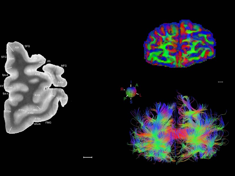
To obtain multimodal datasets from the same specimen, ex vivo MRI and DWI scans (at 7 T and 3 T, respectively) of both hemispheres were collected (Fig. 2A,B) prior to histological processing. For anatomic atlasing, the left hemisphere including the connected brainstem and cerebellum (Fig. 2C) was coronally divided into 2‐cm slabs, and each slab was serially sectioned at 50 µm (Fig. 2D). Every fourth section (200‐µm sampling interval) was stained for Nissl substance (Fig. 2E), and every eighth section was immunostained for NFP (400‐µm interval) or PV (400‐µm interval) to facilitate accurate delineation of the Nissl‐stained sections (Fig. 3A–C). Histological sections were imaged at cellular resolution allowing neuronal soma, dendrites, and axons to be clearly identified (Fig. 2F). A subset of Nissl‐stained sections was selected for detailed anatomical delineation with sampling density higher in regions with greater structural complexity. This strategy enabled adequate sampling of small but functionally critical structures such as the suprachiasmatic nucleus in the hypothalamus (Fig. 4) and the area postrema in the medulla.
Figure 2.
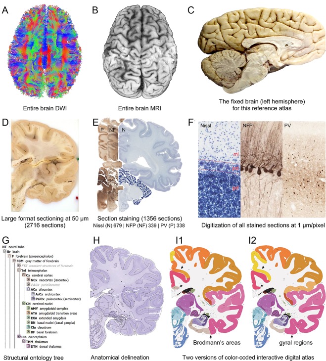
Whole‐brain reference atlas components. A,B: DWI tractography and structural MRI. C: Midline‐sagittal photograph of left hemisphere. D: Block‐face image of a coronal slab. E: Digital images of adjacent sections stained for PV, NFP, and Nissl. F: Cellular‐resolution detail in cerebellar (Nissl and NFP) and cingulate cortex (PV). G: Brain ontology with color codes, acronyms, full names, and hierarchical parent–daughter relationships. H: Anatomical delineation of a Nissl plate from a combined analysis of all three stains. I: Interactive color‐coded digital atlas with both modified Brodmann (I1) and traditional gyral (I2) cortical maps. Black arrows point to some of the differences between these maps.
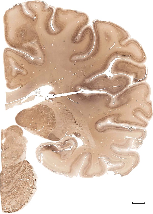
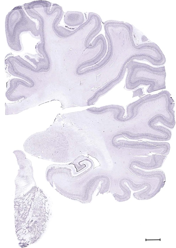
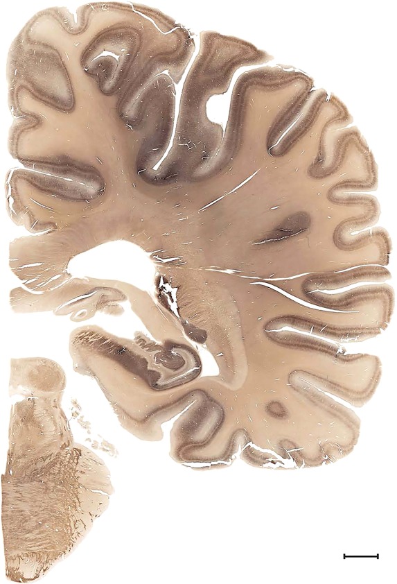
Figure 3.

Examples of closely adjacent whole‐hemisphere sections for the histological stains used in the atlas. A combined analysis of Nissl‐stained (A), and NFP‐ (B) and PV‐ (C) immunostained sections greatly facilitated delineation of both cortical and subcortical regions of the human brain (see examples in Figs. 5, 6, 7). The size of a typical plate at native resolution (1 µm/pixel) is ∼3.0 m wide and 4.3 m high. Scale bar = 3,108 µm in A–C.
Figure 4.

Detailed delineation of the human hypothalamus. A high sampling density (about 40 plates total, with 20 shown here) covering the entire anterior–posterior (A–T) extent of the hypothalamus was employed to ensure sampling and annotation of even the smallest structures such as the suprachiasmatic nucleus (SCN in A–C). For abbreviations see the hypothalamic part of the ontology in Table 3. Scale bar = 1,940 µm in T (applies to A–T).
Creation of a unified structural brain ontology
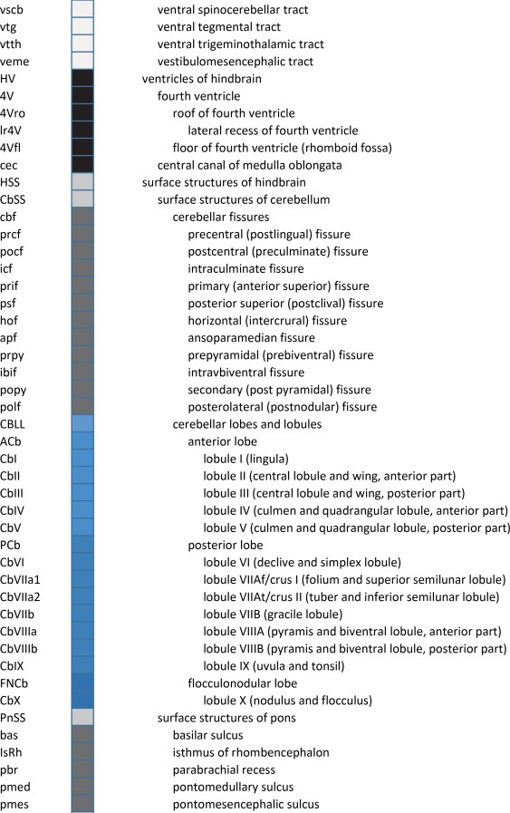
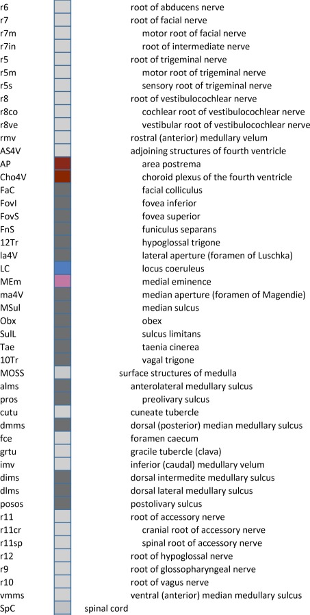
An essential component of modern interactive digital atlases is a unifying hierarchical structural ontology that provides unique IDs (and colors for representation) for each structure in a parent–child architecture. We created a whole‐brain ontology spanning all adult structures (Table 3) and including a developmental axis for transient structures observed during the specification and cytoarchitectural maturation (Miller et al. 2014). The ontology is fundamentally divided into the basic subdivisions of forebrain, midbrain, and hindbrain, further divided into four major branches comprising gray matter, white matter, ventricles, and surface features. For example, daughter structures of “gray matter of forebrain” (Fig. 2G) include the telencephalon, diencephalon, and transient structures of forebrain (e.g., subplate and ventricular zone of the neocortex), while “white matter of forebrain” includes nearly all commissural and long ipsilateral fiber tracts. “Ventricles of forebrain” includes the lateral and third ventricles and related structures, while “surface structures of forebrain” includes important gross landmark features such as cortical gyri and sulci.
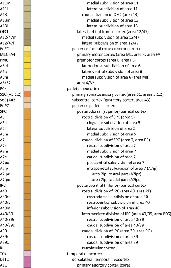
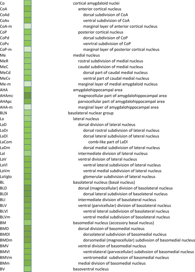
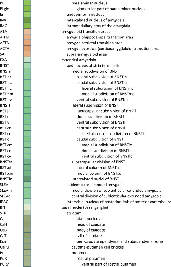
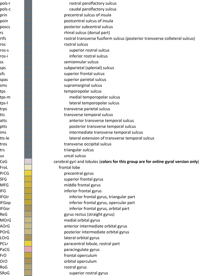
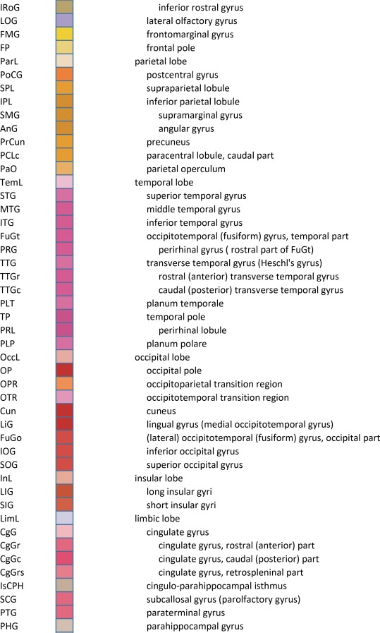
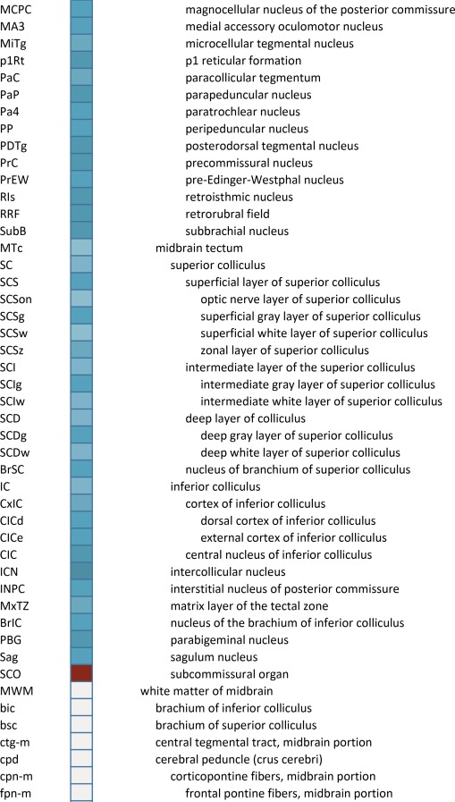
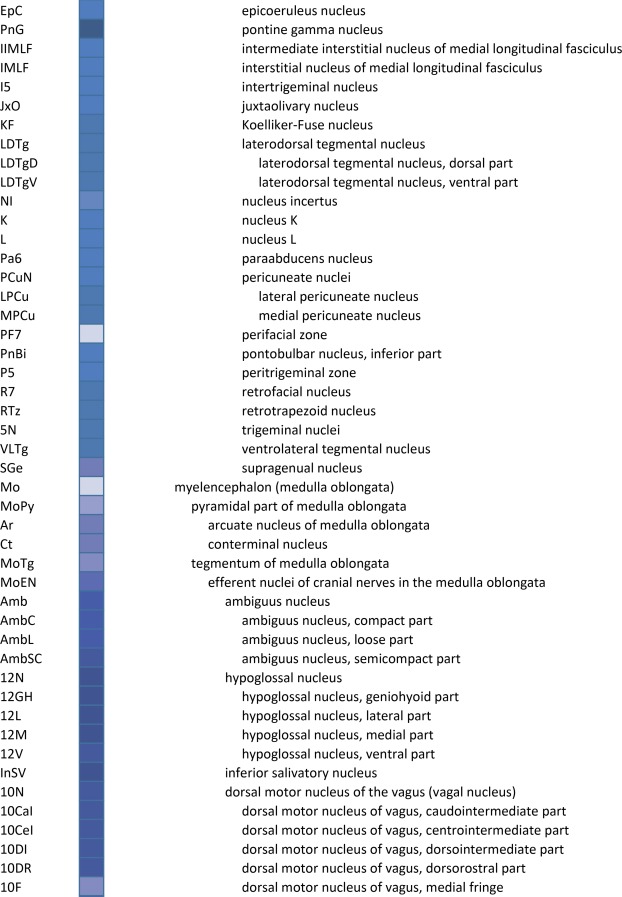
Table 3.
Whole Brain Structure Ontology and Abbreviations

|
|

|

|

|

|

|
|
|

|

|

|

|

|

|

|

|

|

|
|
|

|

|

|
|

|

|

|

|

|
|

|

|

|

|
|
|

|
For cortical structures, we aimed to accommodate both gyral and sulcal parcellation common to neuroimaging studies as well as cytoarchitectural parcellation based on histology, for which two basic terminologies based on Brodmann (Brodmann, 1909) and von Economo (von Economo and Koskinas, 1925; von Economo, 1927) are in usage. We used Brodmann's nomenclature as the primary reference because it is more commonly used, with modifications based on modern literature (see below) and the combined whole‐brain large‐scale cyto‐ and chemoarchitectural analysis here. Specifically, the following sources were used to modify the Brodmann scheme: for the frontal and cingulate cortex: Hof et al. (1995a), Vogt et al. (1995), Vogt et al. (2001), Öngür et al. (2003), Petrides and Pandya (2012), and Vogt and Palomero‐Gallagher (2012); for parietal, temporal, and occipital cortices (mostly changed to Brodmann's terminology where other nomenclature was used): Caspers et al. (2013b), Ding et al. (2009), Ding and Van Hoesen (2010), Scheperjans et al. (2008), Van Essen et al. (2001), Zilles and Amunts (2009), and Goebel et al. (2012). The terminology for the hippocampal formation is derived from Ding and Van Hoesen (2015) and Ding (2013, 2015). For a few cortical areas that Brodmann (1909) did not parcellate in detail (Simić and Hof, 2015), such as posterior parahippocampal areas (areas TH, TL, and TF), we adopted a modified nomenclature from von Ecomono and Koskinas (1925; see Ding and Van Hoesen, 2010). Another example of modification of Brodmann's areas is the orbitofrontal cortex, where Brodmann's large area 11 was replaced with smaller areas 14, 11, and 13 according to a few modern anatomical studies in human (Hof et al., 1995a; Öngür et al., 2003) and our own investigation of Nissl preparations and PV‐ and NFP‐immunostained sections. In addition, some of Brodmann's areas were further subdivided according to recent literature and the analysis here. For instance, Brodmann's areas 22 and 21 (roughly corresponding to von Economo's areas TA and TEd) were subdivided into rostral, intermediate, and caudal parts based on different staining intensity in PV‐stained sections (Ding et al., 2009). Finally, for the insular cortex that was not numbered by Brodmann in human (1909; see Simić and Hof, 2015), three major subdivisions were delineated and these included agranular, dysgranular, and granular insula (e.g., Bauernfeind et al., 2013; Morel et al., 2013), with the latter two further divided into rostral and caudal parts.
Structures from the ontology were delineated as polygons on each Nissl digital image (Fig. 2H), and these structures include both gyral (Fig. 2I1) and modified Brodmann areas (Fig. 2I2) of the neocortex. Together, this comprehensive ontology covers all brain regions and can be used interactively to browse and search delineated structure polygons. It also provides enhanced interlinking capabilities among a broad range of datasets including adult (Hawrylycz et al., 2012) and developing (Miller et al., 2014) human brain transcriptional atlases included in the Allen Brain Atlas (www.brain-map.org).
Delineation of cortical and subcortical gray matter
Anatomical delineation for the 106 selected plates (Fig. 2H) was based on a combined analysis of cyto‐ (Nissl stain) and chemoarchitecture (NFP and PV immunohistochemistry). For example, the boundaries between areas 29 and the neighboring suprasplenial subiculum (SuS) and caudal presubiculum (PrSc; also known as the postsubiculum [PoS]) were confidently identified based on staining features revealed in Nissl‐ (Fig. 5A), and adjacent PV‐ and NFP‐ (Fig. 5B and inset) immunostained sections. Dark NFP and PV immunoreactivity highlights SuS and PrSc, respectively, and these complementary and corroborating data allowed a consensus digital annotation of these regions (Fig. 5C). Similarly, in the ventral temporal neocortex, the border between areas 36 and 20 can be more accurately defined with PV immunostaining than Nissl alone, as area 20 (20i) displays significantly stronger PV immunoreactivity than area 36 (Fig. 5D,E).
Figure 5.

Defining cortical boundaries with a combined analysis of Nissl‐, NFP‐, and PV‐stained sections. A,B, and inset in B: Boundary determining of the indusium griseum (IG), supracallosal subiculum (SuS), retrosplenial areas 29 (A29) and 30 (A30), and caudal presubiculum (PrSc; or postsubiculum [PoS]). C: Color‐coded map of the region shown in A and B. cc, corpus callosum. PV and NFP immunostaining patterns help delineate neocortical borders and white matter tracts. D,E: Differences in PV immunolabeling intensity helps define the boundaries between area 36 and area 20 (20i). Scale bar = 1,106 µm in C (applies to A–C) and E (applies to D,E).
NFP immunoreactivity was in many cases more informative than Nissl stain for delineation of cortical regions based on the selective labeling of pyramidal neuron populations in different layers. For example, many large pyramidal neurons in layer 5 of the primary motor cortex (M1C; Fig. 6A) are NFP‐immunoreactive, while only a small number of medium‐sized neurons are observed in that layer of the primary somatosensory cortex (S1C; Fig. 6B). In contrast, the inferior parietal area (rostrodorsal area 40 [area 40rd], located posterior to S1C; Fig. 6C), has a narrower band of superficial layer labeling and a stronger bilaminar pattern. The combined analysis of Nissl staining and NFP or PV immunolabeling was also useful in defining many subcortical regions and subdivisions such as ventroposterior inferior (VPI), parafascicular (Pf), and centromedian (CM) nuclei in the thalamus (Thal; Fig. 6D) and cranial motor nuclei of the brainstem (Figs. 6E, 7A–C).
Figure 6.
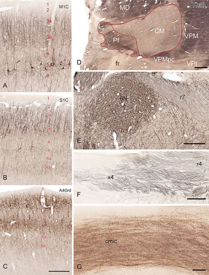
Defining boundaries of cortical and subcortical structures with NFP‐ (A–F) and PV‐ (G) stained sections. A–C: NFP staining patterns in primary motor cortex (M1C), primary somatosensory cortex (S1C), and the rostrodorsal portion of area 40 (A40rd). The locations of these three cortical areas were marked with *, **, and *** respectively in Figure 8A. Arabic numbers specify cortical layers. D: NFP staining pattern in the thalamus (Thal) defines Pf, CM, and adjoining structures. CM, centromedian nucleus; MD, mediodorsal nucleus; Pf, parafascicular nucleus. VPI, ventral posterior inferior nucleus; VPM, ventral posterior medial nucleus; VPMpc, parvocellular part of VPM. E,F: NFP is observed in select white matter tracts in the brainstem including the facial (r7 in E) and trochlear (r4 in F) nerve roots. 6N, abducens nucleus; r7, facial nerve root; x4, decussation of trochlear nerve roots (r4 in F). G: PV is selectively expressed in the commissure of the inferior colliculus (cmic). Scale bar = 777 µm in C (applies to A–C), D, and E; 277 µm in F; 88 µm in G.
Figure 7.
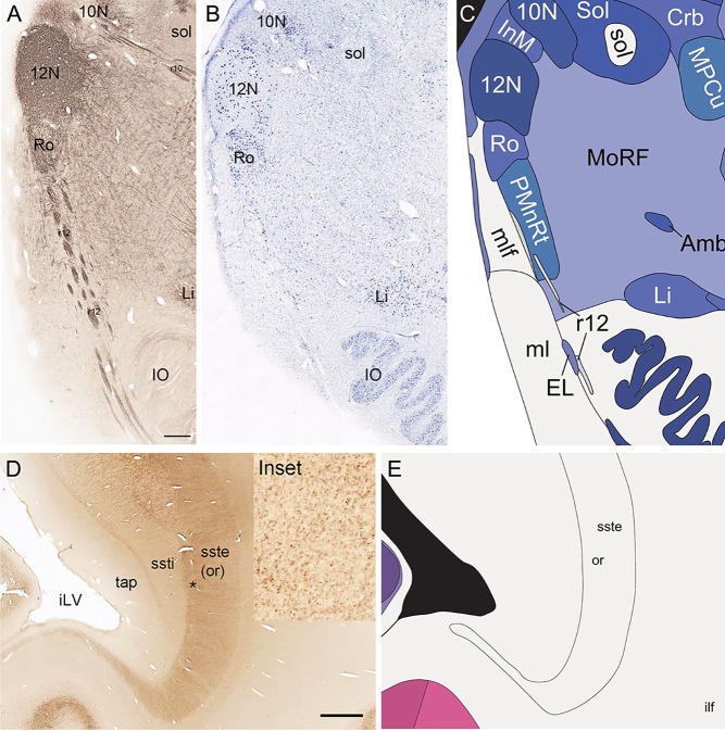
Defining white matter fiber tracts and subcortical structures with combined analysis of NFP and PV stains. A–C: Combined analysis of NFP immunoreactivity (A) and Nissl staining (B) in the medulla leading to anatomical parcellation (C). NFP clearly delineates specific cranial nuclei (e.g., 10N, 12N) and fiber tracts (e.g., r12). D,E: PV‐immunoreactive axons in the external part of sagittal stratum/optic radiation (“or” in D and inset) compared with the internal part of the sagittal stratum (ssti) and tapetum of the corpus callosum (tap) that do not show PV immunoreactivity. Inset: High‐magnification view of PV‐immunoreactive axons in the optic radiation (*). 10N, dorsal motor nucleus of vagus nerve; 12N, hypoglossal nucleus; iLV, inferior horn of the lateral ventricle; IO, inferior olive; r12 and r10, hypoglossal and vagus nerve roots; Scale bar = 777 µm in A (applies to A,B); 1,554 µm in D.
Localization and delineation of white matter tracts
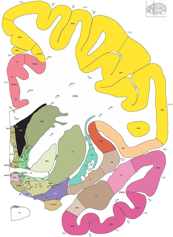
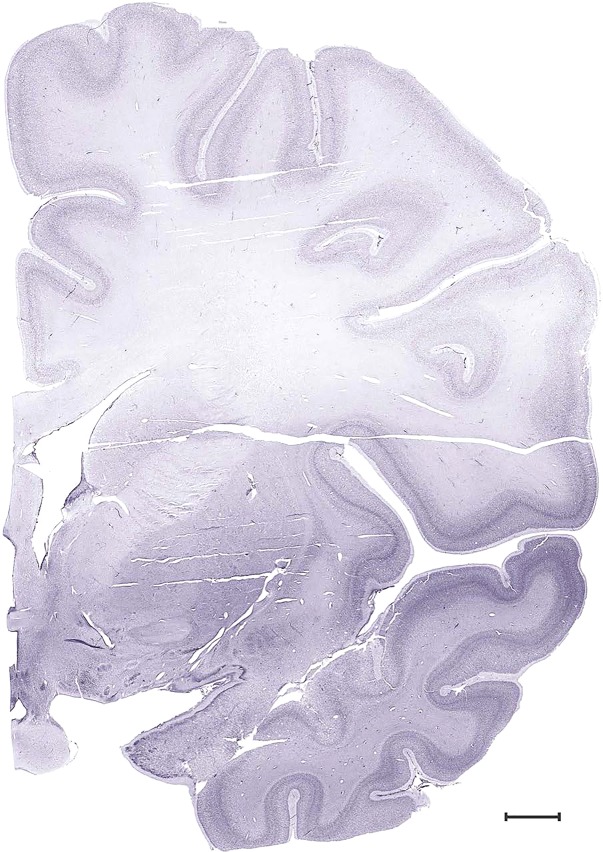
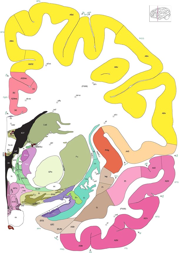
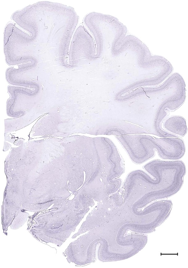
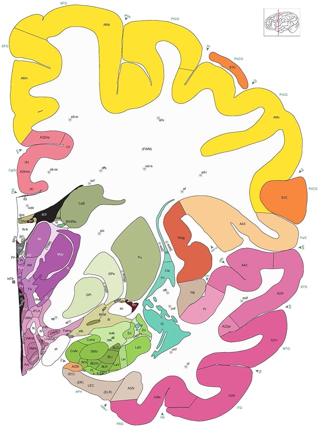
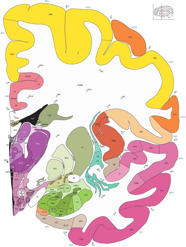
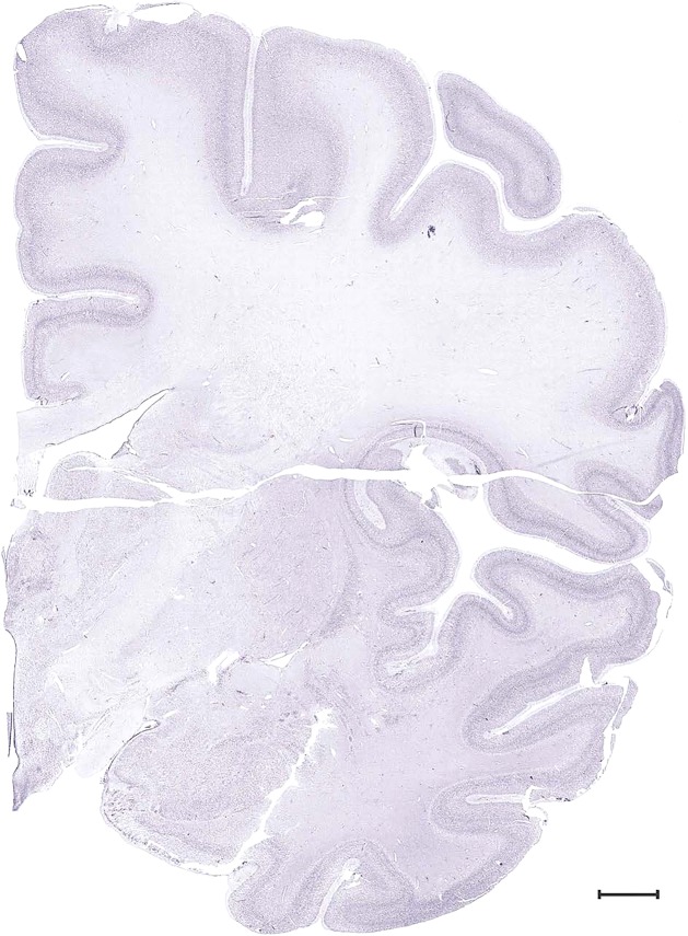
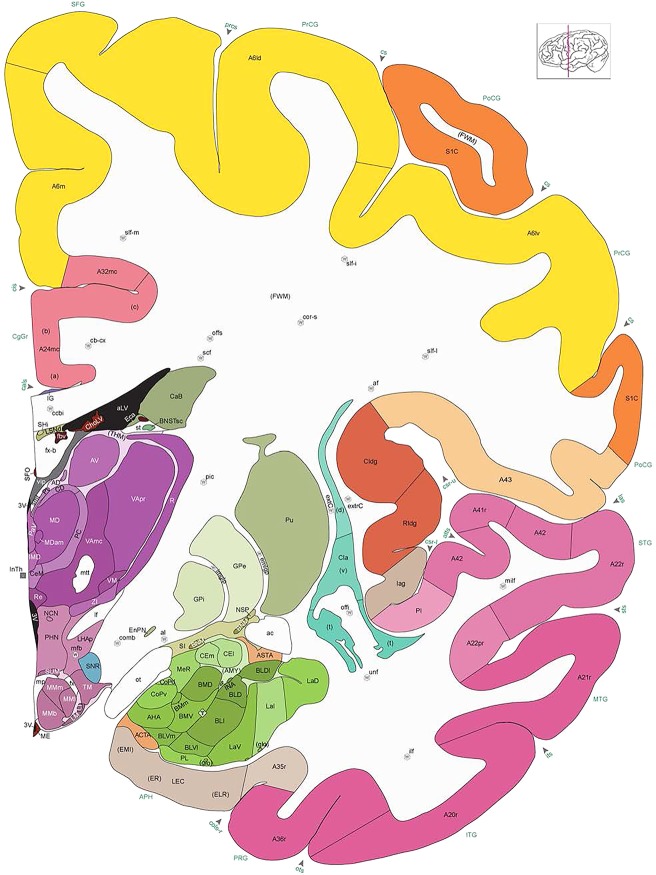
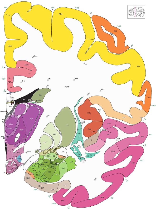
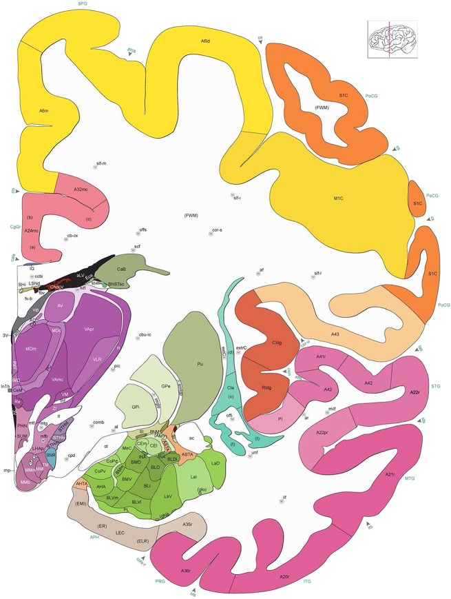
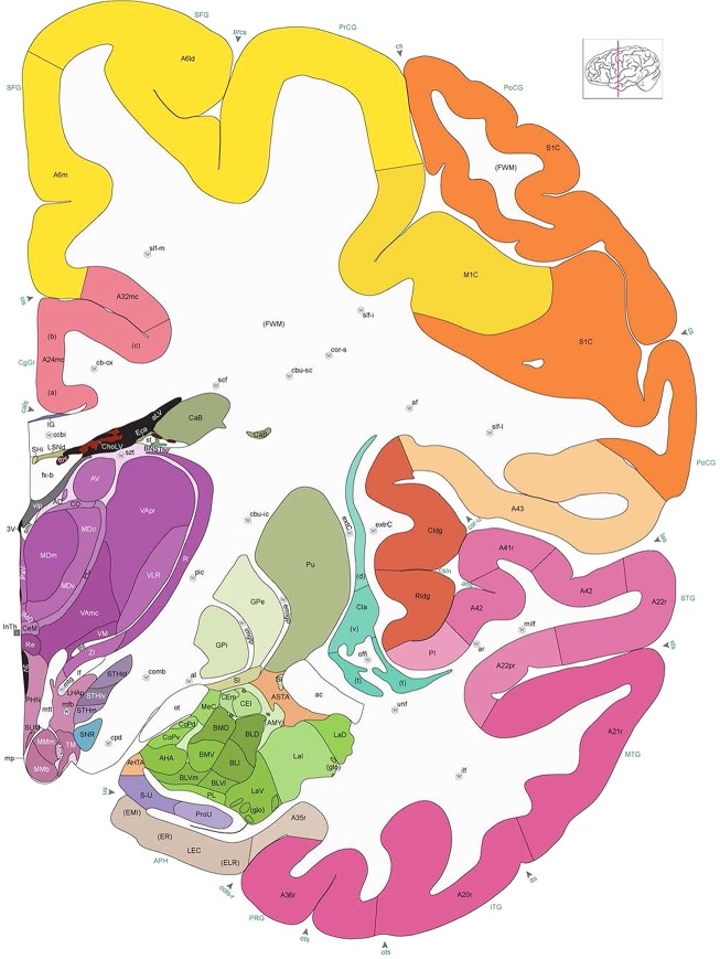
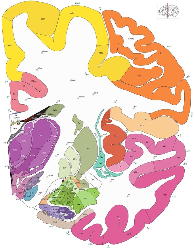
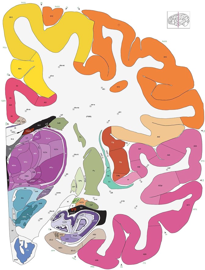
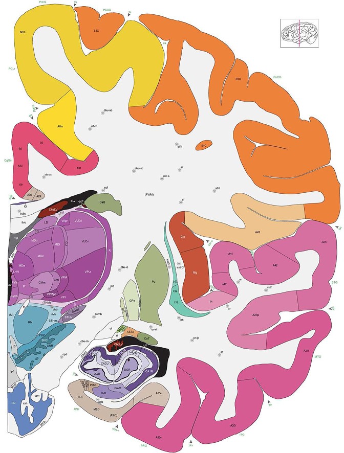
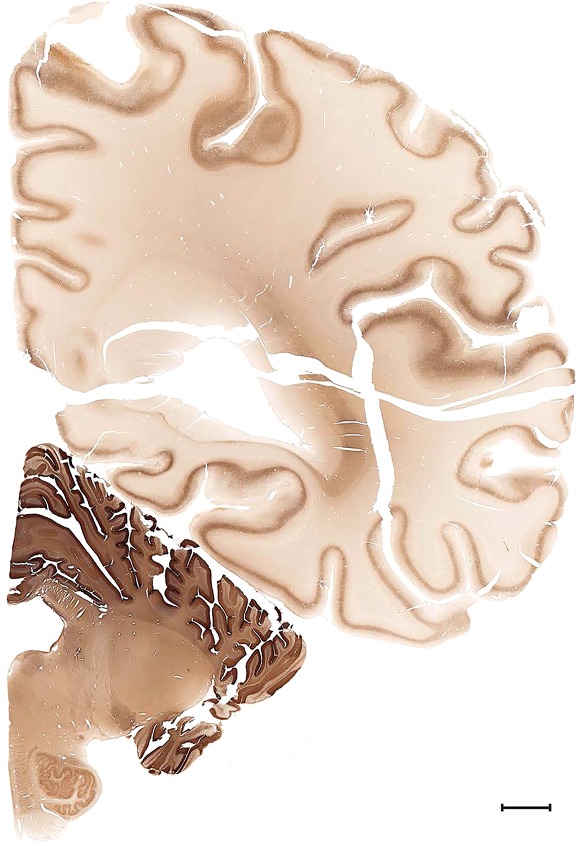
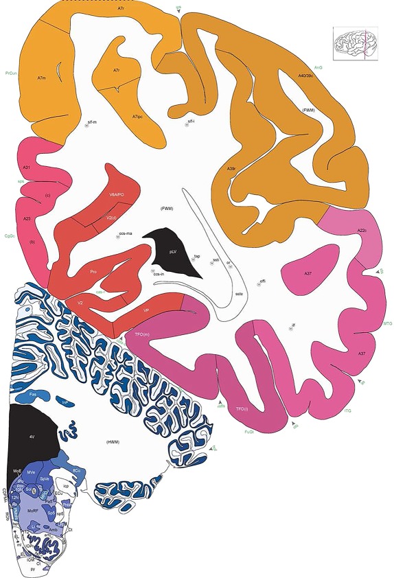
We also aimed for a comprehensive delineation of white matter tracts and cranial nerves (117 total), aided by NFP and PV fiber immunostaining. Motor roots of the cranial nuclei in the brainstem are clearly delineated by NFP staining (Figs. 6E, G, 7A). PV immunoreactivity shows similar discernment of a variety of fiber tracts and trajectories, such as the commissure of the inferior colliculus (Fig. 6F) and the optic radiation (Fig. 7D,E). A representative fully annotated atlas plate is shown in Figure 8A, with complete cyto‐ and chemoarchitecture‐based parcellation and colorization superimposed on the original Nissl image (Fig. 8C). To relate macroscopic (landmarks) and microscopic (histology) cortical anatomy, parallel plates were created with parcellation by gyri and sulci (Fig. 8B) or modified Brodmann areas (Fig. 8A). The denser sampling of subcortical regions allowed comprehensive detailed annotation of fine nuclear architecture for all major regions, as illustrated for the hypothalamus (Fig. 4) and the amygdala (Fig. 9).
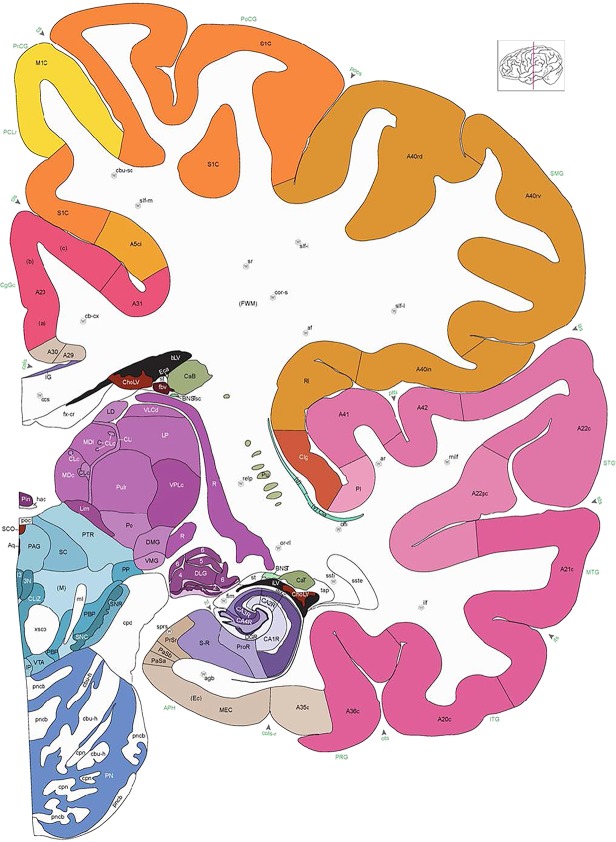
Figure 8.

Alternate schemes for cortical parcellation. Modified Brodmann's areas (A) or sulci and gyri (B) were annotated on the same Nissl‐stained plate (C) to show micro‐ and macrostructural relationships. Examples of how cortical areas were delineated are given in Figures 5 and 6. The markers (*, **, ***) and (#) in A indicate the locations of pictures in Figure 6A–C and Figure 5D,E, respectively. For abbreviations see the ontology in Table 3. Inset is a schematic representation of the whole hemisphere based on MRI, with the red vertical lines in A and B indicating the location of the section plate. Both modified Brodmann's areas and gyral/sulcal mapping of the cerebral cortex are available online at www.branspan.org. Scale bar = 3,108 µm in A–C.
Figure 9.

Detailed parcellation of the human amygdalar complex. Shown are ten of the 18 annotated plates covering the A‐P extent (A–J) of the amygdala. For abbreviations see the amygdalar portion of the ontology in Table 3 Scale bar = 3,102 µm in J (applies to A–J).
Identification of novel brain subregions
In addition to confirming previously identified structures, the combination of high image resolution and dense (200‐µm‐interval) Nissl sampling made it possible to reveal or clarify a number of complex or smaller brain structures, while the linkage to the Allen Human Brain Atlas (Hawrylycz et al., 2012) allowed corroboration of these structures with other gene expression data. One example is in the mediodorsal nucleus (MD) of the thalamus, where we observed a group of densely packed larger cells between the paraventricular nucleus (PaV) and the main portion of the MD, which we named the anteromedial subdivision of the MD (MDam in Fig. 10A). In situ hybridization data of both acetylcholinesterase (ACHE) and neurotensin (NTS) supports this partition, as they are selectively enriched in this region compared with the main part of the MD (Fig. 10B and inset). Similarly, we identified a novel subdivision of the basomedial nucleus (BM) of the amygdala. This subdivision is located medial to the dorsal and ventral subdivisions of the BM (BMD and BMV) and was termed BMm (medial subdivision of BM; Fig. 10C and inset). The BMm displays enriched cellular expression of the γ‐aminobutyric acid (GABA) receptor subunit E (GABRE) compared with the neighboring BMD and BMV (Fig. 10D). The homologs of MDam and BMm in other species have not been reported.
Figure 10.

Novel subdivisions of the mediodorsal nucleus (MD) of the thalamus and basomedial nucleus (BM) of the amygdala. A: Nissl staining reveals a group of larger cells (termed MDam, labeled with * in high magnification image and overview atlas plate (inset)) located between the paraventricular nucleus (PaV) and anterior mediodorsal nucleus MDm) of the thalamus distinct from neighboring regions. B: Distinct molecular specificity of MDam is demonstrated by ISH for ACHE and NTS (inset in B). C,D: Novel subdivision of amygdalar basomedial nucleus differentiated by smaller and relatively lightly Nissl‐stained cells (termed BMm, labeled with * in high magnification image and overview atlas plate (inset) in C) and selective enrichment for the GABA receptor subunit E (GABRE, in D) compared with neighboring dorsal and ventral regions (BMD and BMV) and posterior cortical nucleus (CoP). Scale bar = 1,109 µm in B (applies to A,B); 1,550 µm in D (applies to C,D).
Another new area was identified running along the side of lateral olfactory stria, situated medially to the piriform cortex (Pir) and laterally to the substantia innominata (SI). This was termed the lateral olfactory area (LOA) and was found to have distinct histological features from the neighboring Pir and SI (Fig. 11). Compared with the Pir, the LOA does not have a dark, densely packed layer 2 on Nissl stain and has much stronger NFP immunoreactivity. In Nissl‐stained materials, the SI contains many cellular patches of differing sizes, packing densities, and staining intensities, with cells of contrasting shapes and sizes, compared with the LOA (Fig. 11A). In sections immunostained for NFP, only the largest neurons are labeled (Fig. 11B). The SI does not display laminar organization, while the LOA has a clear but discontinuous layer 2 and one deep layer. In contrast, the Pir has a dark and continuous layer 2 and a less darkly stained layer 3.
Figure 11.

Identification of the lateral olfactory area (LOA) in the adult human brain. A,B: Adjacent sections stained for Nissl (A) and NFP (B) showing the architectural features of LOA that differ from neighboring substantia nominata (SI) and piriform cortex (Pir). In Nissl‐stained sections, SI contains different types of cell patches (asterisks and arrowhead) while Pir is characterized by a darkly stained and densely packed layer 2 (A). LOA does not have these characteristic features, but shows cell patches that are different from those in SI (A). In NFP‐immunostained sections, Pir is very light throughout while LOA shows strong labeling in the superficial layer (B). Only the large‐celled patch (arrow) and scattered large cells of SI are strongly stained while other patches are negative (B). ac, anterior commissure; NDBh, horizontal part of nucleus of diagonal band; VeP, ventral pallidus; lost, lateral olfactory stria. Scale bar = 430 µm in A (applies to A,B).
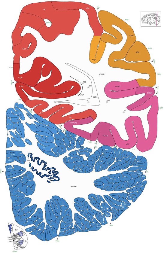
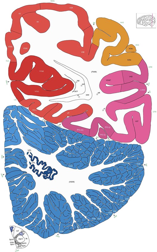
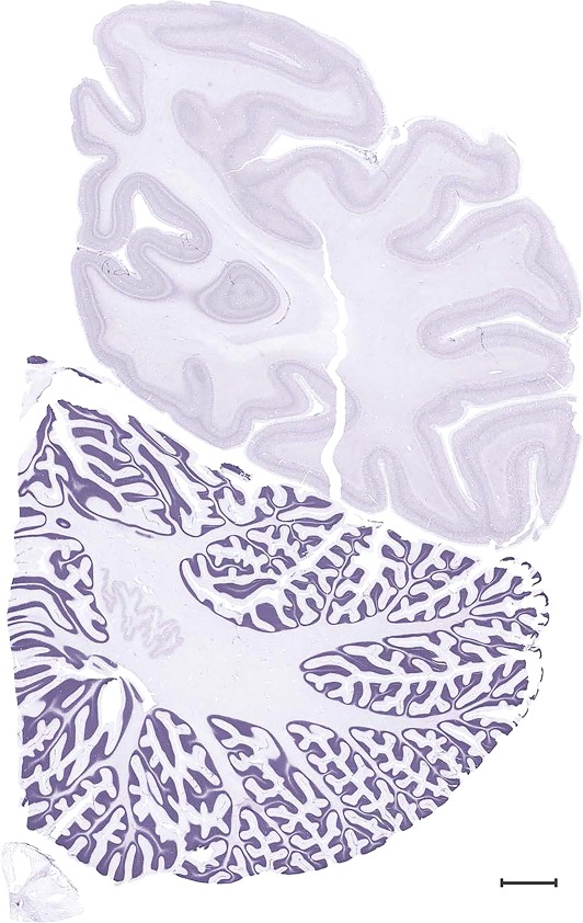
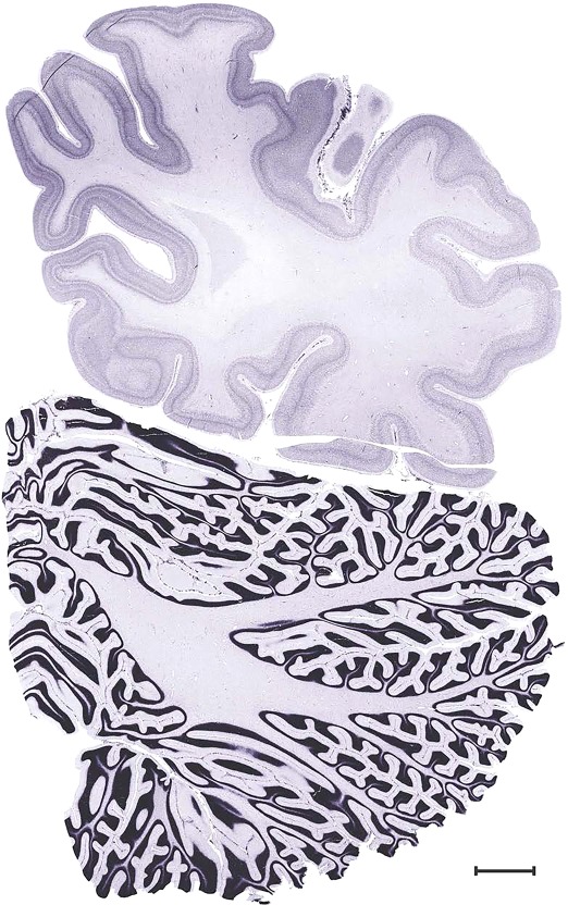
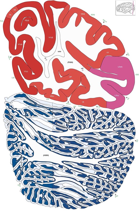
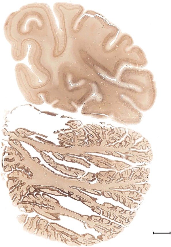
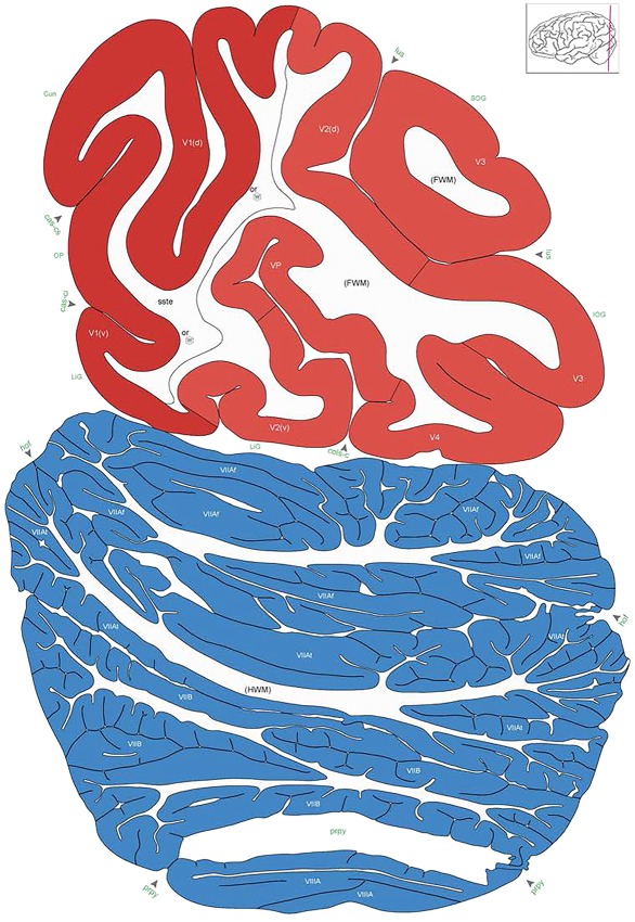
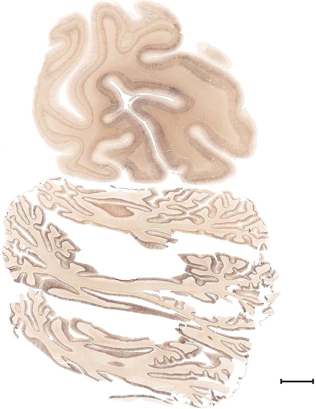
Two other structures described previously only in non‐human primates were identified as well, such as area prostriata (APro) and the basal interstitial nucleus of the cerebellum (BIcb). APro is a region located at the junction of the retrosplenial, post‐ and parasubiculum, posterior cingulate, and anterior–dorsal primary visual cortices. It has been described in detail in macaque monkey (Morecraft et al., 2000; Ding et al., 2003) and is important for fast procession of peripheral vision (Yu et al., 2012). Although its existence in the human brain was briefly described, its exact location and extent has not been reported in detail so far. Our mapping indicates that APro is much larger in human (Fig. 12) than in macaque monkey (Ding et al., 2003). The BIcb in the human brain is located deep to the medial interpositus nucleus (InPM; globose nucleus) of the cerebellum and consists of scattered large NFP‐immunoractive neurons (Fig. 13).
Figure 12.

Location and topographic relationship of area prostriata (APro). APro (labeled as Pro) is adjoined by the retrosplenial cortex (areas 29 and 30, not shown), postsubiculum (PoS in A), posterior cingulate cortex (area 23 in B–D) anterodorsally, and dorsal secondary visual cortex (V2d in D‐G) posterodorsally. Anteroventrally, APro is adjoined by the ventral secondary visual cortex (V2 in A–D). Posteroventrally and posteriorly, APro is adjoined by the anteroventral part of the primary visual cortex (V1v in E–H). Scale bar = 4,420 µm in H (applies to A–H).
Figure 13.
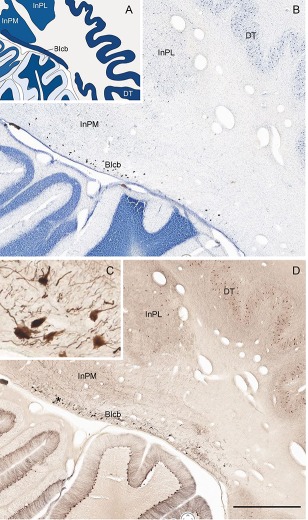
A novel subregion of the deep nuclei of the cerebellum. This has been named the basal interstitial nucleus of cerebellum (BIcb) and is embedded deep in the white matter medial to the dentate nucleus (DT) and lateral and inferior to the globose nucleus (i.e., the medial interpositus nucleus [InPM in A]). In Nissl stain, the cells in the BIcb are large and darkly stained (B). In NFP stain, these large cells are positively stained (C,D; C is the higher power view of the “*” region in D). Scale bar = 1,554 µm in D (applies to B,D).
Identifying anatomical landmarks in MRI data
Transposing the Nissl‐based anatomical delineations into full 3D annotations registered to the accompanying MRI volume is challenging due to the incomplete and nonuniform sampling of those annotations. However, individual Nissl plates can be matched to corresponding planes of the MRI data to allow the identification of features of specific structures that can then be mapped onto MRI data from other brains without accompanying architecture‐based delineations. The utility of this approach can be demonstrated in the case of the medial geniculate nucleus (MG) and the dorsal lateral geniculate nucleus (DLG). A comparison of the architecture‐based atlas (Fig. 14A) and the corresponding MRI plate (Fig. 14B) from the same brain shows that the MG has high and the DLG low signal intensity. Combining these features with basic spatial topography, the MG and DLG in the MRI scans from other brains from the Allen Human Brain Atlas (Hawrylycz et al., 2012) are clearly discerned (Fig. 14C,D). The MG is so similar in signal intensity to the adjoining white matter (consistently high signal intensity in T1‐weighted images) that it would probably be misidentified as white matter if the extracted feature (i.e., high signal intensity) was not used. With the topography of the histology‐based parcellation as a guide, many fine structures can be similarly identified in MRI data that would otherwise be difficult to identify and discriminate, thus extending the value of this single brain atlas to the interpretation of neuroimaging data (Fig. 15).
Figure 14.

Identification of fine anatomical features in same‐brain MRI and transfer to other brain MRI data. A: Reference atlas plate showing subdivisions of the medial geniculate nucleus (MG), dorsal lateral geniculate nucleus (DLG), and adjoining regions. B: Identification of the MG and DLG on the ex vivo MRI scan from the same brain by comparison with the corresponding reference plate based on subtle differences between MRI signal intensity of the MG and DLG and neighboring white and gray matter. The majority of the image contrast comes from T2* weighting and the contrast has been inverted. C,D: Identification of the MG and DLG on the MRI scans (T1 images) from other brains in the Allen Human Brain Atlas without histological stains using the extracted features of MG (bright) and DLG (dark) signal intensity at the same sectioning plane as the atlas. Hip, hippocampus; IP, interpeduncular nucleus; MD, mediodorsal thalamic nucleus; PAG, periaqueductal gray; Pul, pulvinar; SN, substantia nigra. Scale bar = 5,160 µm in D (applies to B–D).
Figure 15.

Structure identification on MRI of other brains. A–D: Identification of structures on T1‐weighted MRI scans from case H0351.2002 of the Allen Human Brain Atlas (http://human.brain-map.org). By virtue of anatomical features extracted from this reference atlas (see Fig. 14), structures such as Pu, GPe (A), MD, RN, SN, ZI (B), Pul, MG, DLG (C), and “or” (optic radiation, D) are consistently identified. E,F: Pul, MG, DLG, SN, RN, ZI, and other structures were also confirmed in a T1‐weighted MRI dataset from another case (H0351.2001). For abbreviations see the ontology in Table 3. Scale bar = 5,160 µm in A (applies to A–F).
Whole‐brain histology‐based atlas with corresponding MRI and DWI
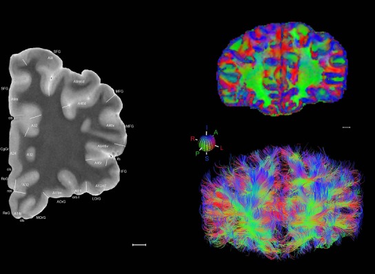
The complete set of histology‐based atlas plates is presented in Figures 16 and 17. These include a plate locator (Fig. 16) marking the A‐P sampling locations of all 106 annotated atlas plates and selected corresponding Nissl‐stained and adjacent NFP and PV immunohistological plates (Fig. 17). To translate the atlas structural delineations onto the MRI dataset, a set of 76 coronal MRI slices at 2‐mm intervals (Fig. 18) from the same hemisphere was selected and annotated (Fig. 19, left column). Macroscopic landmarks such as cortical sulci and gyri were used as guides to match histological and MRI planes of section, and local topography was used (e.g. see Figs. 14, 15) to label identifiable structures including all neocortical areas and major subcortical regions.
Figure 16.
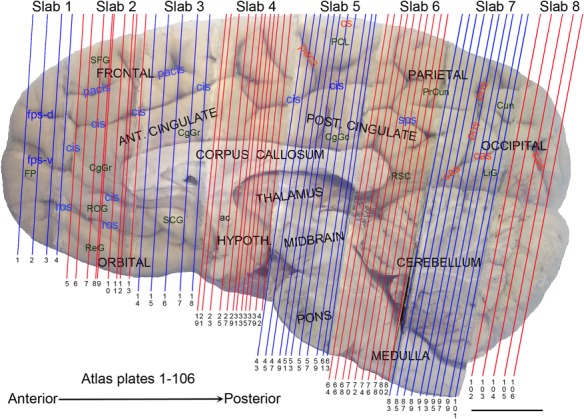
Anteroposterior position of the 106 annotated plates shown in Figure 17. Major macroscopic landmarks (sulci and gyri) on the medial aspect of the left hemisphere are indicated (flipped to show the plate levels (plates 1–106) in an anterior‐to‐posterior order). General locations of slabs 1–8 were also marked at the top. Note that in slabs 4–7, only the alternative plates were indicated, to avoid busy lines. For abbreviations see Table 3. Scale bar = 2 cm.
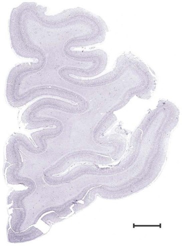
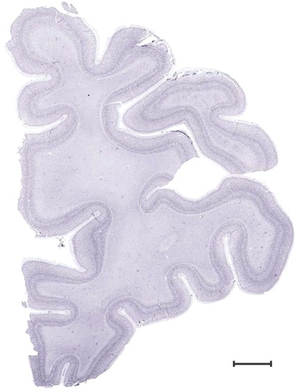
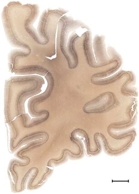
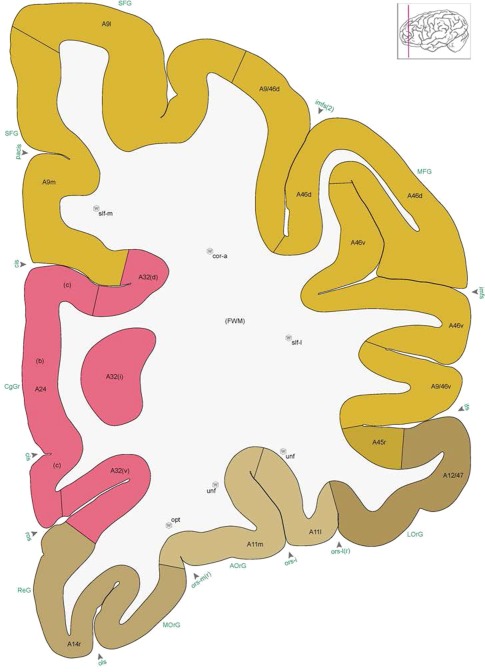
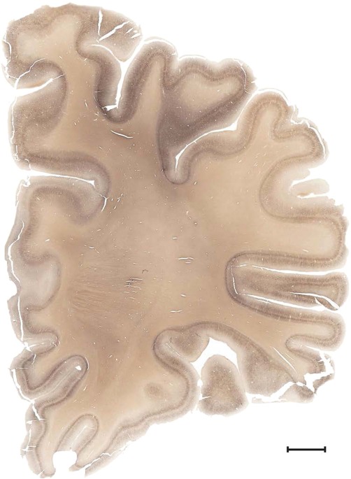
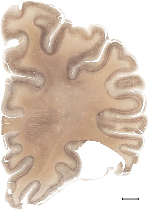
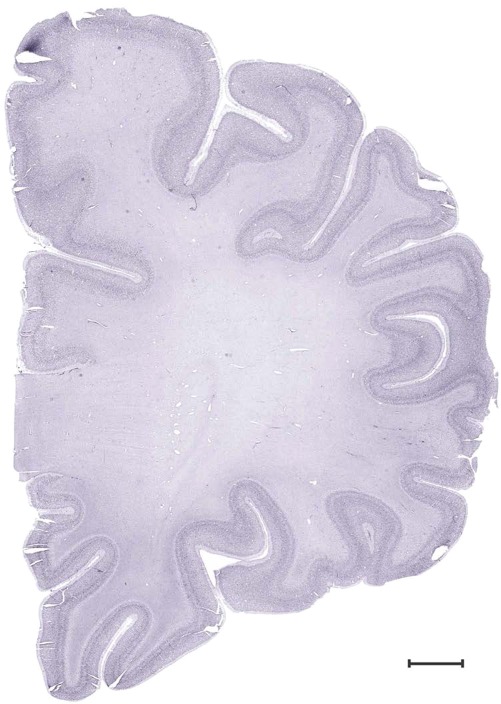
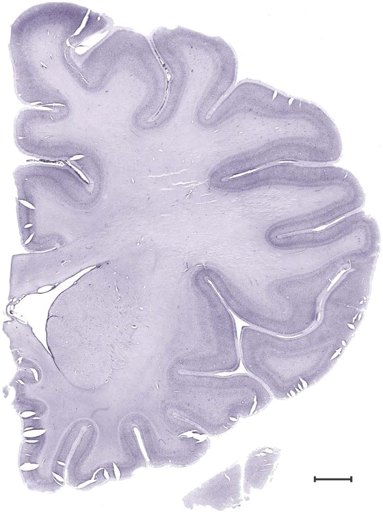
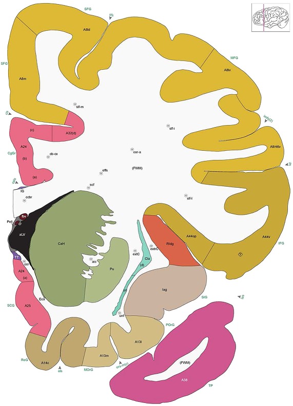
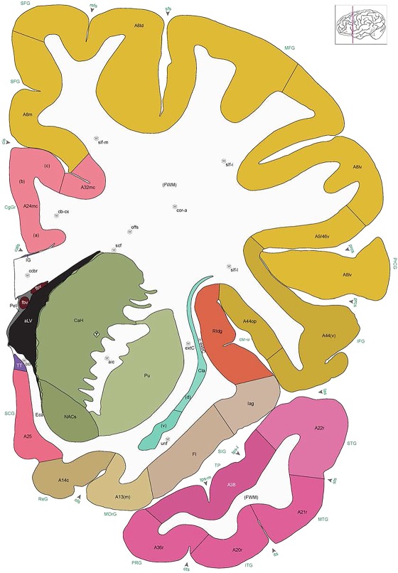
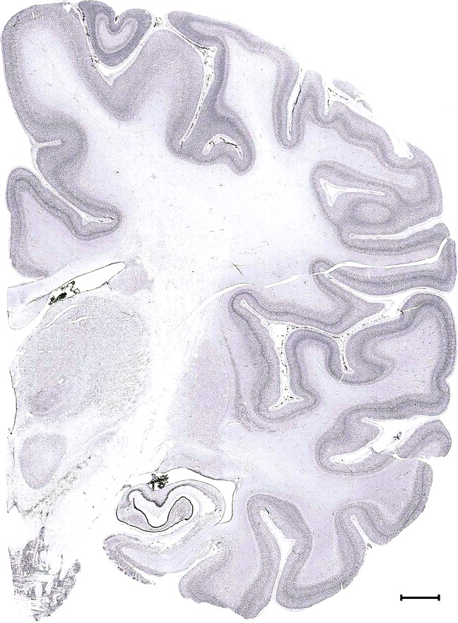
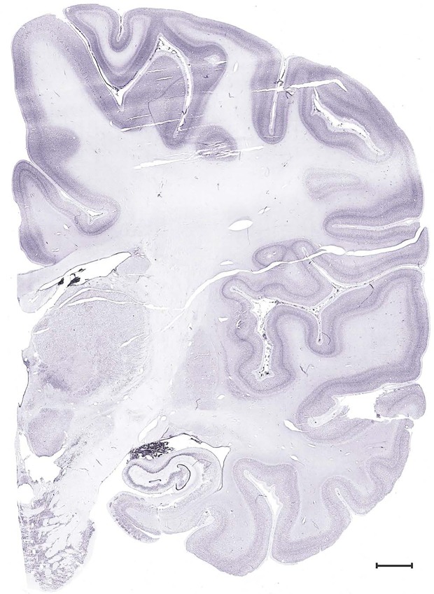
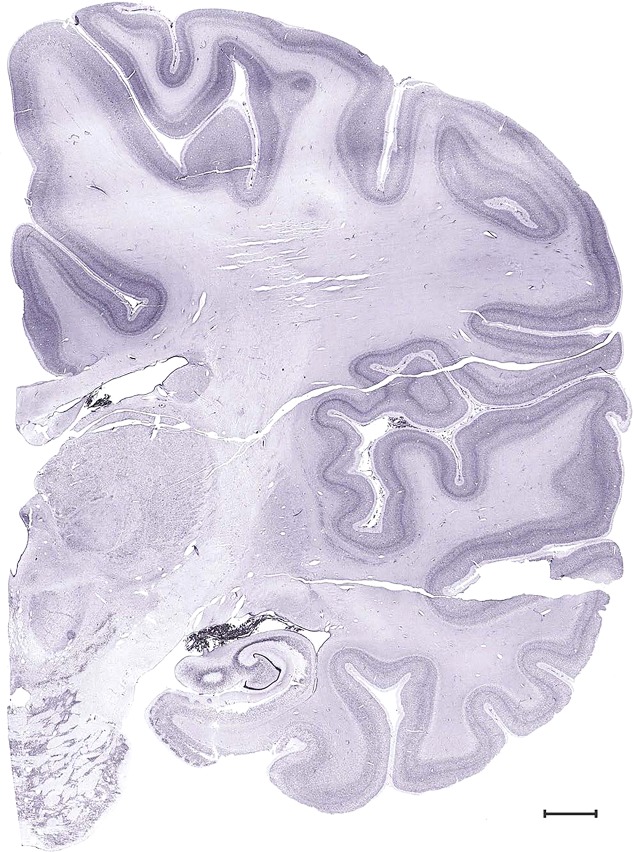
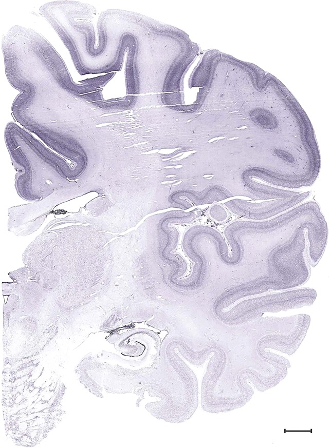
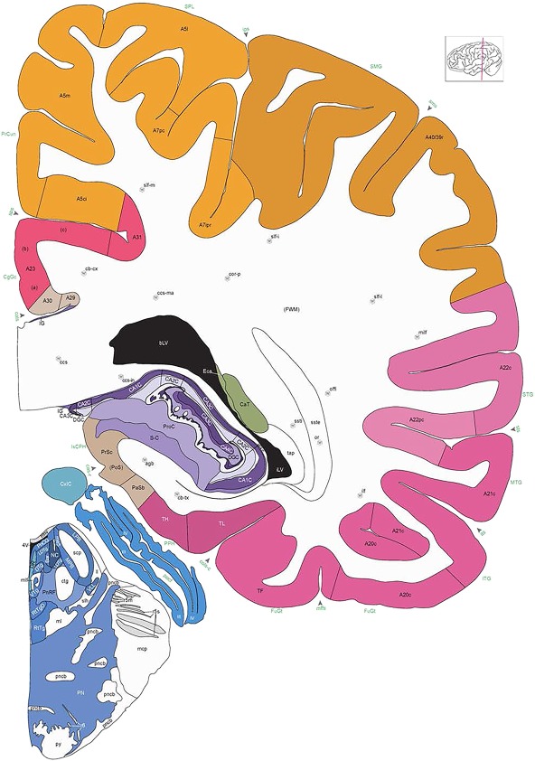
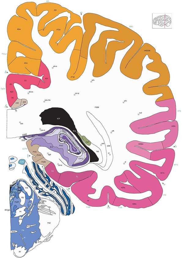
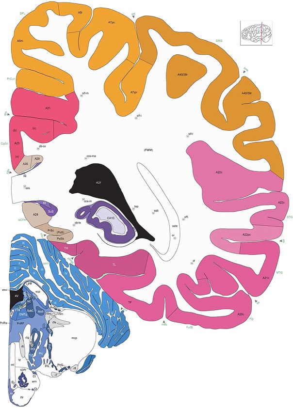
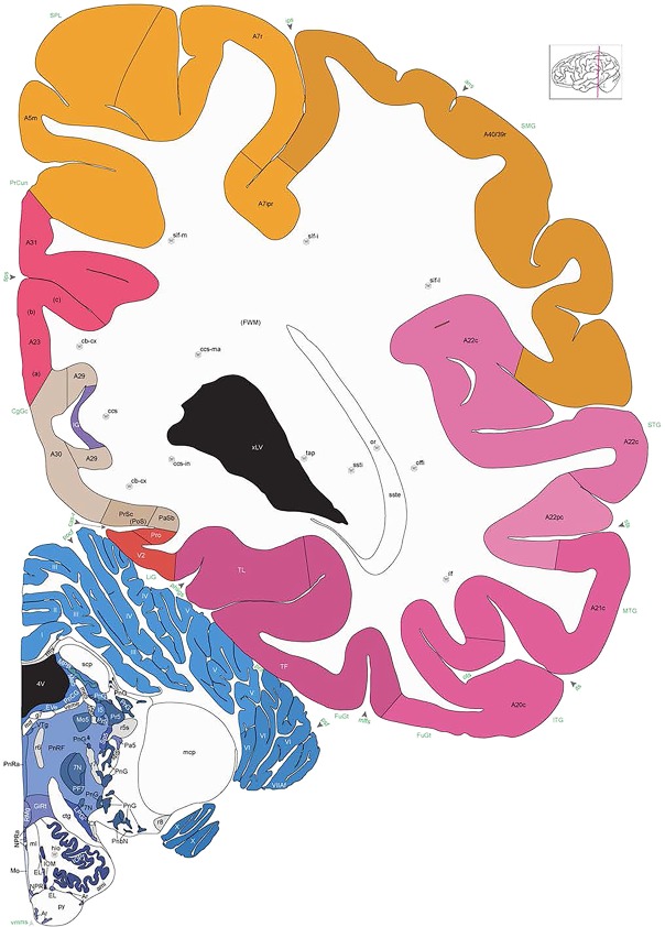
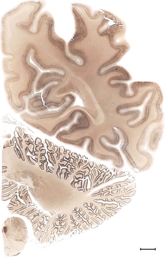
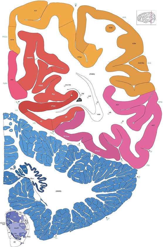
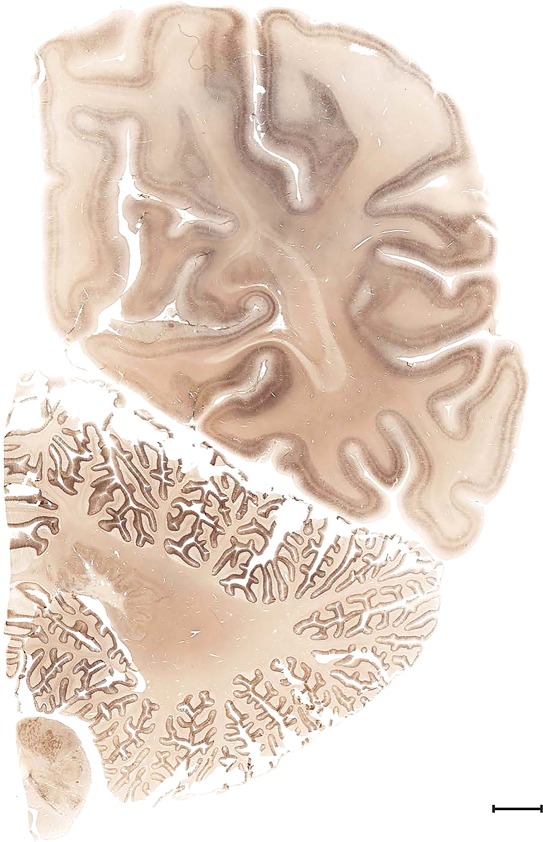
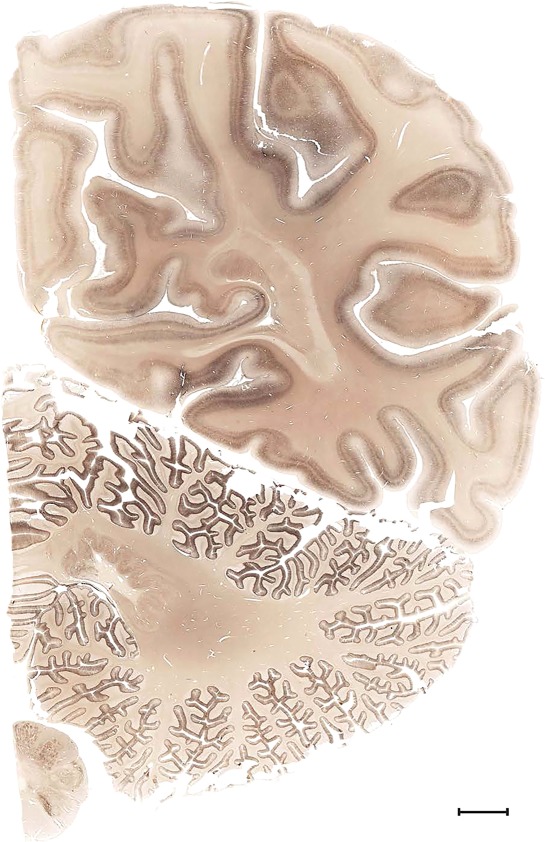
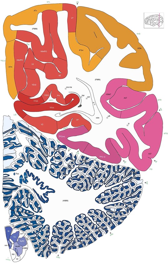
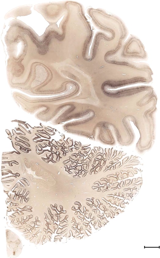
Figure 17.

Level 1a (01_111)
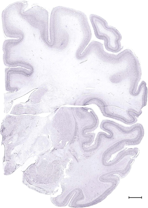
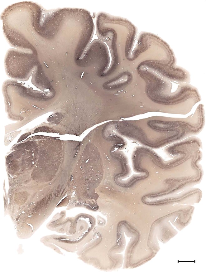
Human brain atlas plates. 106 plates with matching histological sections are displayed in anterior‐to‐posterior (A‐P) order. The matching histological images include 50 Nissl‐stained, and 50 NFP‐ and 6 PV‐immunostained sections. The 106 plate images, corresponding to the A‐P positions delineated in Figure 16, combine the cortical annotation of modified Brodmann areas and traditional gyri and sulci. At the top right of each plate, plate levels (levels 1–106, as indicated in Fig. 16), as well as slab numbers and section positions in that slab (e.g., 01–111 represents the 111th section of slab 1) are indicated. At each level, a color‐coded atlas plate (“a” series; 1a–106a) and a histological image (“b” series; 1b–106b) are presented. The inset diagram at the top right corner of each atlas plate shows the A‐P position (red line) of that plate on a schematic representation of the whole hemisphere based on MRI. The green lettering along the cortical surface indicates cortical sulci (lower case, often with black arrowheads) and gyri (upper case), which were generally defined by adjacent sulci. Modified Brodmann areas were labeled within the cortical gray matter with differential color coding. In plates containing cerebellar cortex, alternative plates were annotated for three cerebellar cortical zones (vermis, paravermis, and lateral hemisphere) and 10 lobules (lobules I–X), respectively. Other subcortical structures were also labeled with differential color coding. The general locations of most white matter tracts are indicated by a circled “W”. Fiber tracts with clear boundaries, such as ac, mtt, ot, sste/or, fx, fr, scp, py, and ml, were outlined by black lines without color code (white). The parcellation and subdivisions of different brain regions as well as the parent–daughter relationship and abbreviation of each structure are detailed in Table 3. Note that two separate versions of this atlas for modified Brodmann areas and traditional gyri and sulci, respectively, are available in the online version of this atlas (www.brainspan.org or http://brainspan.org/static/atlas). For abbreviations see Table 3. Scale bar = 5 mm (at levels 1b–106b).
Figure 18.

Gross anatomy of the left hemisphere and anteroposterior position of the 76 annotated MRI images shown in Figure 19. Main macroscopic landmarks (sulci and gyri) on dorsal (A), lateral (B), and ventral (C) aspects of the left hemisphere are indicated. The A‐P locations (levels 1–76) of the 76 MRI images are marked with black lines 1–76 in B. * and # indicate two corresponding regions. For abbreviations see Table 3. Scale bar = 2 cm in A (applies to A–C).
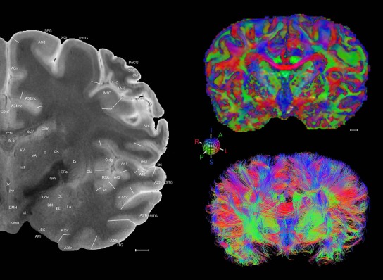
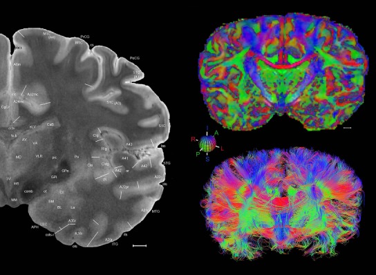
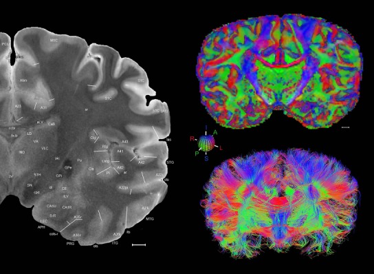
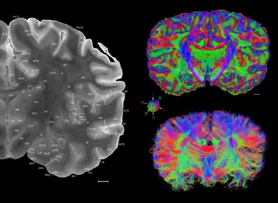
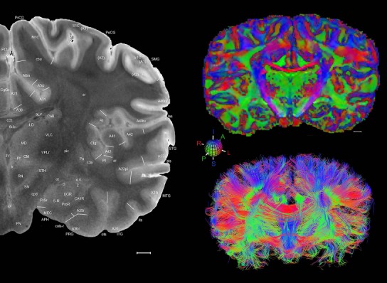
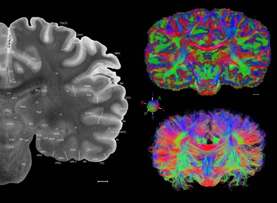
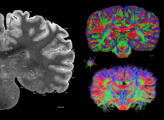
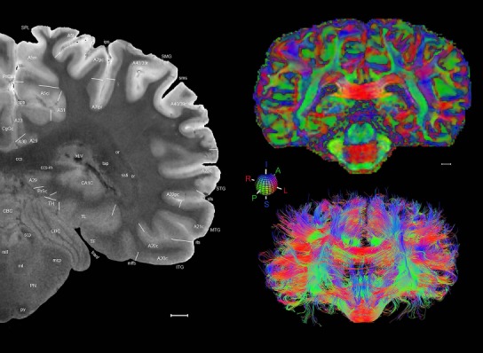
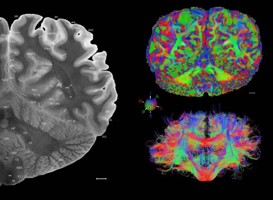
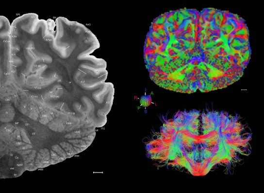
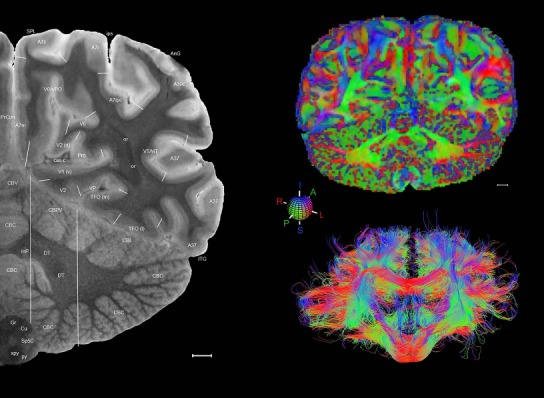
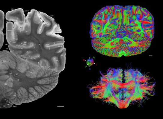
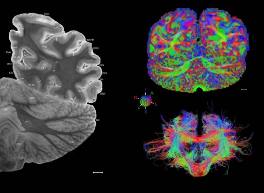
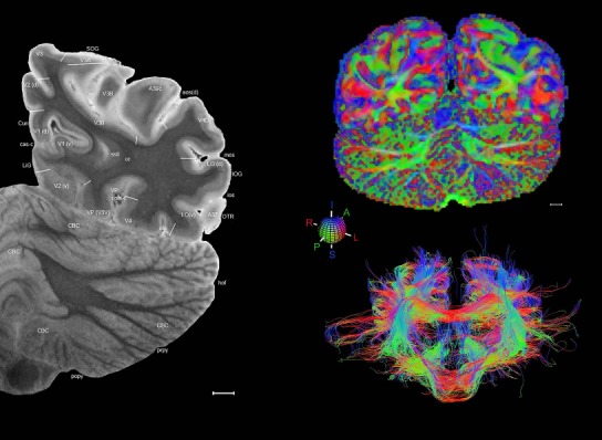
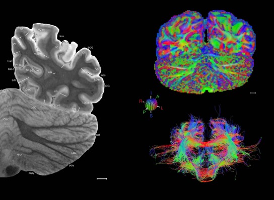
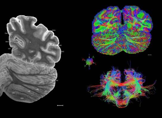
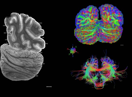
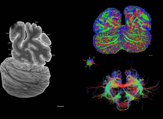
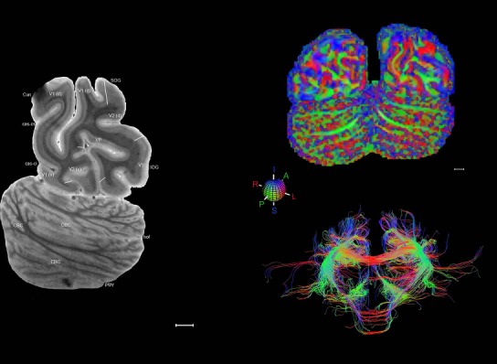
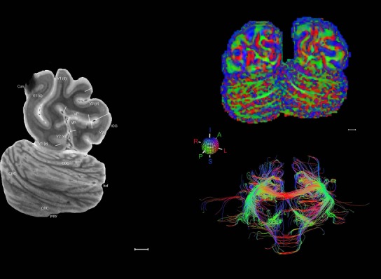
Figure 19.

Level 01
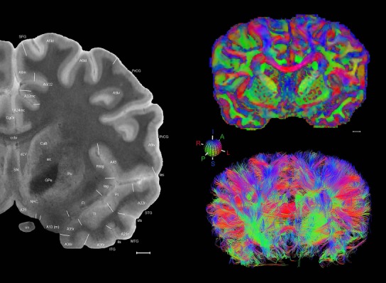
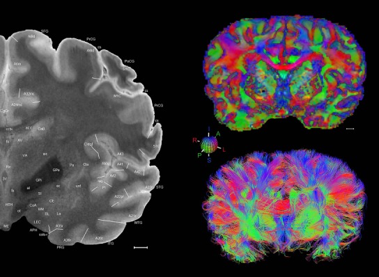
MRI and DWI plates from the same brain. Left column: Seventy‐six sequential 7T MRI slices from the same left hemisphere as the atlas shown in Figure 17 were annotated according to the atlas plates in Figure 17. The interval between each slice is 2 mm. The MRI images were annotated for easily predicted and/or identified structures through correspondence to the annotated histological atlas. Several clearly delineated fiber tracts are annotated as well, including the optic radiation (“or” at levels 42–69) and somatosensory radiation (‘sr” at levels 38–46). For abbreviations see Table 3. Right column: Top panel shows colorized fractional anisotropy (FA) maps of the corresponding plane of section in the DWI dataset, representing the primary eigenvectors of the diffusion tensor data overlaid on the FA map. Bottom panel shows tractography images created in TrackVis showing all tracts passing through the represented plane of section (90% of tracts omitted with only tracts longer than 20 mm displayed). Scale bar = 5 mm.
Figure 17.

Level 1b (NFP (SMI‐32))
Figure 17.

Level 2a (01_179)
Figure 17.
Level 2b (Nissl)
Figure 17.

Level 3a (01_247)
Figure 17.

Level 3b (NFP (SMI‐32))
Figure 17.

Level 4a (01_307)
Figure 17.
Level 4b (Nissl)
Figure 17.

Level 5a (02_111)
Figure 17.

Level 5b (NFP (SMI‐32))
Figure 17.

Level 6a (02_111)
Figure 17.
Level 6b (NFP (SMI‐32))
Figure 17.
Level 7a (02_175)
Figure 17.

Level 7b (Nissl)
Figure 17.

Level 8a (02_219)
Figure 17.

Level 8b (NFP (SMI‐32))
Figure 17.

Level 9a (02_231)
Figure 17.

Level 9b (NFP (SMI‐32))
Figure 17.

Level 10a (02_295)
Figure 17.

Level 10b (Nissl)
Figure 17.

Level 11a (02_335)
Figure 17.
Level 11b (NFP (SMI‐32))
Figure 17.

Level 12a (02_359)
Figure 17.
Level 12b (NFP (SMI‐32))
Figure 17.

Level 13a (02_407)
Figure 17.
Level 13b (Nissl)
Figure 17.

Level 14a (03_031)
Figure 17.

Level 14b (Parvalbumin)
Figure 17.

Level 15a (03_095)
Figure 17.

Level 15b (Nissl)
Figure 17.

Level 16a (03_159)
Figure 17.
Level 16b (Nissl)
Figure 17.
Level 17a (03_227)
Figure 17.

Level 17b (Nissl)
Figure 17.
Level 18a (03_291)
Figure 17.

Level 18b (Nissl)
Figure 17.

Level 19a (04_035)
Figure 17.

Level 19b (Nissl)
Figure 17.

Level 20a (04_051)
Figure 17.

Level 20b (NFP (SMI‐32))
Figure 17.

Level 21a (04_059)
Figure 17.

Level 21b (Nissl)
Figure 17.
Level 22a (04_083)
Figure 17.

Level 22b (Nissl)
Figure 17.

Level 23a (04_095)
Figure 17.

Level 23b (NFP (SMI‐32))
Figure 17.

Level 24a (04_115)
Figure 17.
Level 24b (Nissl)
Figure 17.
Level 25a (04_135)
Figure 17.

Level 25b (NFP (SMI‐32))
Figure 17.

Level 26a (04_147)
Figure 17.

Level 26b (Nissl)
Figure 17.

Level 27a (04_167)
Figure 17.

Level 27b (NFP (SMI‐32))
Figure 17.

Level 28a (04_179)
Figure 17.
Level 28b (Nissl)
Figure 17.

Level 29a (04_195)
Figure 17.

Level 29b (NFP (SMI‐32))
Figure 17.
Level 30a (04_207)
Figure 17.

Level 30b (Nissl)
Figure 17.

Level 31a (04_215)
Figure 17.

Level 31b (NFP (SMI‐32))
Figure 17.
Level 32a (04_231)
Figure 17.

Level 32b (Nissl)
Figure 17.

Level 33a (04_239)
Figure 17.
Level 33b (Nissl)
Figure 17.

Level 34a (04_251)
Figure 17.

Level 34b (Nissl)
Figure 17.
Level 35a (04_259)
Figure 17.

Level 35b (NFP (SMI‐32))
Figure 17.
Level 36a (04_267)
Figure 17.
Level 36b (Nissl)
Figure 17.

Level 37a (04_279)
Figure 17.

Level 37b (NFP (SMI‐32))
Figure 17.
Level 38a (04_291)
Figure 17.

Level 38b (Nissl)
Figure 17.
Level 39a (04_307)
Figure 17.

Level 39b (NFP (SMI‐32))
Figure 17.

Level 40a (04_315)
Figure 17.

Level 40b (Nissl)
Figure 17.
Level 41a (04_327)
Figure 17.

Level 41b (NFP (SMI‐32))
Figure 17.

Level 42a (04_335)
Figure 17.

Level 42b (Nissls)
Figure 17.

Level 43a (05_031)
Figure 17.

Level 43b (Nissl)
Figure 17.

Level 44a (05_047)
Figure 17.

Level 44b (Nissl)
Figure 17.

Level 45a (05_063)
Figure 17.
Level 45b (NFP (SMI‐32))
Figure 17.
Level 46a (05_079)
Figure 17.

Level 46b (NFP (SMI‐32))
Figure 17.
Level 47a (05_091)
Figure 17.

Level 47b (NFP (SMI‐32))
Figure 17.

Level 48a (05_103)
Figure 17.
Level 48b (Nissl)
Figure 17.

Level 49a (05_123)
Figure 17.
Level 49b (Nissl)
Figure 17.

Level 50a (05_135)
Figure 17.

Level 50b (NFP (SMI‐32))
Figure 17.

Level 51a (05_147)
Figure 17.
Level 51b (Nissl)
Figure 17.

Level 52a (05_159)
Figure 17.

Level 52b (Nissl)
Figure 17.

Level 53a (05_171)
Figure 17.
Level 53b (Nissl)
Figure 17.

Level 54a (05_187)
Figure 17.

Level 54b (NFP (SMI‐32))
Figure 17.
Level 55a (05_203)
Figure 17.

Level 55b (Nissl)
Figure 17.

Level 56a (05_223)
Figure 17.

Level 56b (Nissl)
Figure 17.

Level 57a (05_235)
Figure 17.

Level 57b (NFP (SMI‐32))
Figure 17.

Level 58a (05_255)
Figure 17.

Level 58b (NFP (SMI‐32))
Figure 17.

Level 59a (05_275)
Figure 17.

Level 59b (NFP (SMI‐32))
Figure 17.

Level 60a (05_287)
Figure 17.
Level 60b (NFP (SMI‐32))
Figure 17.

Level 61a (05_303)
Figure 17.

Level 61b (Parvalbumin)
Figure 17.

Level 62a (05_311)
Figure 17.

Level 62b (NFP (SMI‐32))
Figure 17.

Level 63a (05_323)
Figure 17.
Level 63b (Nissl)
Figure 17.

Level 64a (06_035)
Figure 17.

Level 64b (Parvalbumin)
Figure 17.

Level 65a (05_047)
Figure 17.

Level 65b (Nissl)
Figure 17.

Level 66a (06_063)
Figure 17.
Level 66b (NFP (SMI‐32))
Figure 17.

Level 67a (06_083)
Figure 17.

Level 67b (Nissl)
Figure 17.
Level 68a (06_095)
Figure 17.

Level 68b (NFP (SMI‐32))
Figure 17.
Level 69a (06_107)
Figure 17.

Level 69b (Parvalbumin)
Figure 17.

Level 70a (06_119)
Figure 17.

Level 70b (NFP (SMI‐32))
Figure 17.

Level 71a (06_131)
Figure 17.

Level 71b (Nissl)
Figure 17.
Level 72a (06_147)
Figure 17.

Level 72b (Parvalbumin)
Figure 17.

Level 73a (06_159)
Figure 17.

Level 73b (NFP (SMI‐32))
Figure 17.
Level 74a (06_179)
Figure 17.

Level 74b (NFP (SMI‐32))
Figure 17.

Level 75a (06_195)
Figure 17.

Level 75b (Nissl)
Figure 17.

Level 76a (06_207)
Figure 17.

Level 76b (NFP (SMI‐32))
Figure 17.

Level 77a (06_223)
Figure 17.
Level 77b (Parvalbumin)
Figure 17.

Level 78a (06_239)
Figure 17.

Level 78b (Nissl)
Figure 17.

Level 79a (06_255)
Figure 17.

Level 79b (NFP (SMI‐32))
Figure 17.

Level 80a (06_271)
Figure 17.

Level 80b (NFP (SMI‐32))
Figure 17.
Level 81a (06_291)
Figure 17.

Level 81b (NFP (SMI‐32))
Figure 17.

Level 82a (06_299)
Figure 17.

Level 82b (Nissl)
Figure 17.

Level 83a (07_027)
Figure 17.

Level 83b (Nissl)
Figure 17.

Level 84a (07_043)
Figure 17.
Level 84b (NFP (SMI‐32))
Figure 17.

Level 85a (07_059)
Figure 17.

Level 85b (NFP (SMI‐32))
Figure 17.
Level 86a (07_075)
Figure 17.

Level 86b (Nissl)
Figure 17.

Level 87a (07_091)
Figure 17.
Level 87b (NFP (SMI‐32))
Figure 17.

Level 88a (07_111)
Figure 17.
Level 88b (NFP (SMI‐32))
Figure 17.
Level 89a (07_123)
Figure 17.

Level 89b (Nissl)
Figure 17.

Level 90a (07_147)
Figure 17.

Level 90b (NFP (SMI‐32))
Figure 17.

Level 91a (07_163)
Figure 17.

Level 91b (NFP (SMI‐32))
Figure 17.

Level 92a (07_171)
Figure 17.

Level 92b (Nissl)
Figure 17.

Level 93a (07_191)
Figure 17.
Level 93b (NFP (SMI‐32))
Figure 17.
Level 94a (07_207)
Figure 17.

Level 94b (NFP (SMI‐32))
Figure 17.

Level 95a (07_223)
Figure 17.

Level 95b (Nissl)
Figure 17.
Level 96a (07_235)
Figure 17.

Level 96b (NFP (SMI‐32))
Figure 17.

Level 97a (07_251)
Figure 17.

Level 97b (Nissl)
Figure 17.

Level 98a (07_267)
Figure 17.

Level 98b (NFP (SMI‐32))
Figure 17.

Level 99a (07_287)
Figure 17.
Level 99b (Nissl)
Figure 17.

Level 100a (07_299)
Figure 17.

Level 100b (Nissl)
Figure 17.

Level 101a (07_315)
Figure 17.

Level 101b (NFP (SMI‐32))
Figure 17.

Level 102a (08_039)
Figure 17.
Level 102b (Nissl)
Figure 17.
Level 103a (08_103)
Figure 17.
Level 103b (NFP (SMI‐32))
Figure 17.
Level 104a (08_167)
Figure 17.

Level 104b (Nissl)
Figure 17.

Level 105a (08_231)
Figure 17.
Level 105b (NFP (SMI‐32))
Figure 17.

Level 106a (08_291)
Figure 17.

Level 106b (Nissl)
Some well‐known white matter tracts such as the optic radiation (“or” in Fig. 19, levels 42–69) and auditory radiation (“ar”) are clearly visible in the 7 T MRI images and can be clearly followed for a long distance due to their darker appearance than the surrounding white matter. Interestingly, a corresponding part of the somatosensory radiation (named here the “sr”) is also clearly visible (Fig. 19, levels 38–46). The “sr” is normally treated as part of the superior radiation in the literature and mainly originates from the ventroposterior lateral nucleus of the thalamus and targets the primary somatosensory cortex. In this 7 T MRI dataset, like the “or” and “ar,” the “sr” is observed to stand out from surrounding white matter and thus deserves an independent term (i.e., somatosensory radiation) as do optic and auditory radiations.
Figure 19.

Level 02
Figure 19.

Level 03
Figure 19.
Level 04
Figure 19.

Level 05
Figure 19.

Level 06
Figure 19.

Level 07
Figure 19.

Level 08
Figure 19.

Level 09
Figure 19.

Level 10
Figure 19.

Level 11
Figure 19.

Level 12
Figure 19.
Level 13
Figure 19.

Level 14
Figure 19.

Level 15
Figure 19.

Level 16
Figure 19.

Level 17
Figure 19.

Level 18
Figure 19.

Level 19
Figure 19.

Level 20
Figure 19.

Level 21
Figure 19.

Level 22
Figure 19.

Level 23
Figure 19.

Level 24
Figure 19.

Level 25
Figure 19.

Level 26
Figure 19.

Level 27
Figure 19.

Level 28
Figure 19.

Level 29
Figure 19.
Level 30
Figure 19.

Level 31
Figure 19.

Level 32
Figure 19.

Level 33
Figure 19.
Level 34
Figure 19.
Level 35
Figure 19.

Level 36
Figure 19.
Level 37
Figure 19.
Level 38
Figure 19.

Level 39
Figure 19.
Level 40
Figure 19.
Level 41
Figure 19.

Level 42
Figure 19.

Level 43
Figure 19.

Level 44
Figure 19.
Level 45
Figure 19.

Level 46
Figure 19.
Level 47
Figure 19.

Level 48
Figure 19.

Level 49
Figure 19.

Level 50
Figure 19.
Level 51
Figure 19.

Level 52
Figure 19.

Level 53
Figure 19.

Level 54
Figure 19.

Level 55
Figure 19.

Level 56
Figure 19.

Level 57
Figure 19.
Level 58
Figure 19.
Level 59
Figure 19.
Level 60
Figure 19.

Level 61
Figure 19.
Level 62
Figure 19.

Level 63
Figure 19.

Level 64
Figure 19.

Level 65
Figure 19.
Level 66
Figure 19.
Level 67
Figure 19.
Level 68
Figure 19.
Level 69
Figure 19.

Level 70
Figure 19.
Level 71
Figure 19.

Level 72
Figure 19.
Level 73
Figure 19.
Level 74
Figure 19.
Level 75
Figure 19.

Level 76
Finally, color‐coded orientation maps and tractography maps of both hemispheres from the same brain are also available and are presented in Figure 19 (right column). By comparison with the accompanying MRI plates, some white matter fiber tracts can be identified. For example, at level 40 of Figure 19, the callosal and cingulate bundles, superior longitudinal fasciculus (slf‐m, slf‐I, and slf‐l), and somatosensory radiation can be easily localized with the guide of the annotated MRI atlas.
For convenience Figures 16‐19 are presented, together with Table 3, after the literature list at the end of the paper.
DISCUSSION
Brain reference atlases are essential resources for neuroscience research, serving to identify and annotate the complex anatomical architecture of the brain and allow communication across laboratories and various research disciplines attempting to link structure to function (Fischl et al., 1999; Toga et al., 2006; Amunts et al., 2007; Evans et al., 2012). Ideally, modern digital atlases should comprise 3D reference frameworks with comprehensive anatomical coverage and cellular resolution cyto‐ and chemoarchitectural histology‐based structural annotation using hierarchical ontologies, and correlated histological and neuroimaging data (Toga et al., 2006; Destrieux et al., 2010; Evans et al., 2012; Caspers et al., 2013a). All currently available human brain reference atlases lack some of these features (see Table 1), mainly due to the large size and structural complexity of the human brain and the resource‐intensive and technology‐limiting nature of the endeavor (Amunts et al., 2013). We sought to fill this gap by generating a fully annotated, high‐resolution anatomical reference atlas for a complete adult female human brain as an open access community resource. The atlas consists of brain‐wide neuroimaging (MRI, DWI) and histological data (Nissl, NFP, PV) based on whole‐hemisphere serial sectioning, staining, and true cellular resolution imaging. Most importantly, the atlas is comprehensively annotated using a unified hierarchical structural ontology based on combined cyto‐ and chemoarchitectural parcellation of 862 gray matter and white matter structures. A freely accessible online atlas browser was created to allow easy visualization and navigation, and the resource is integrated with other human brain cellular resolution gene expression and transcriptomic atlases (Hawrylycz et al., 2012; Miller et al., 2014).
Parcellation of the human neocortex presents a particular challenge, as several different schemes based on cortical gyri and sulci or histological delineation are in common usage (Brodmann, 1909; Talairach and Tournoux, 1988; Fischl et al., 2004; Duvernoy, 1999; Damasio, 2005; Mai et al., 2008; Destrieux et al., 2010; Petrides, 2012), and the relationship between cortical geometry and architectonic identity is variable across the cortex (Fischl et al., 2008). To serve both communities, we chose to perform multiple annotations of the same dataset. The first is based on macroscopic annotation of gyri and sulci, while the second is based on microscopic analysis of combined cyto‐ and chemoarchitectural data to create a modified Brodmann parcellation. This unique human dataset of interleaved Nissl staining, and NFP and PV immunolabeling in a whole hemisphere, allowed a complete parcellation based on variations in overall cell density, NFP immunolabeling of subsets of long‐range excitatory projection neurons, and PV‐expressing neurons and neuropil. In many cases this parcellation agrees with those generated using other techniques such as receptor autoradiography and Nissl‐based gray‐level indices (Zilles and Amunts, 2009; Amunts et al., 2010; Vogt et al., 2013). For example, the inferior parietal lobule has been consistently divided into three basic regions based on cellular and receptor architecture (Caspers et al., 2013b), and our analysis of cyto‐ and chemoarchitecture corroborates this tripartite delineation (albeit with a different nomenclature). In many other cases these data allowed a detailed parcellation of regions that had not yet been examined in detail by others, such as the area prostriata and other structures described above. In principle, this dataset could be reannotated by other researchers to provide alternate interpretations. Finally, this dataset could be aligned to new functional parcellations based on neuroimaging data, such as a recent analyses from the Human Brainnetome Atlas (Fan et al., 2016) and the Human Connectome Project (www.humanconnectome.org; Glasser et al., 2016), opening up new possibilities for linking cytoarchitecture and function at microscopic and macroscopic scales.
There is a fundamental schism between probabilistic reference atlases used in neuroimaging (Hammers et al., 2003; Ahsan et al., 2007; Scheperjans et al., 2008; Shattuck et al., 2008; Diedrichsen et al., 2009; Kuklisova‐Murgasova et al., 2011), based on thousands of individuals, and detailed histological reference atlases based on exhaustive analysis and annotation of single representative brain specimens (Brodmann, 1909; von Economo and Koskinas, 1925; Sarkisov et al., 1955). It is not currently possible to analyze large numbers of whole brains histologically and thus build a probabilistic histological atlas, although strong efforts are under way to move in the direction of generating probabilistic histological reference atlases using standard histological (JuBrain; Caspers et al., 2013a) as well as novel imaging techniques (Magnain et al., 2014, 2015; Wang et al., 2014; Zilles et al., 2016). Furthermore, human brains exhibit a remarkable amount of interindividual variability, particularly in the gyri and sulci of the cerebral cortex (Mazziotta et al., 2001; Uylings et al., 2005; Toga et al., 2006; Amunts et al., 2007; Ding and Van Hoesen, 2010; Zilles and Amunts, 2010, 2013). For instance, one brain may have area 35 located in the medial bank of a deep collateral sulcus (CoS), while another may have its area 35 in the lateral bank of a shallow CoS, or even the crown of the anterior fusiform gyrus (Ding and Van Hoesen, 2010). Thus it is not realistically meaningful to map histological annotations from a single specimen directly into a probabilistic reference space, even with advances in techniques for deformable registration. On the other hand, the current generation of both MRI and DWI data in the same specimen as the histological data allows the direct correlation of cytoarchitectural features with MRI features or landmarks. As we demonstrate, this dataset may thus allow feature extraction that can be applied to other brains to identify fine anatomical structures not otherwise identifiable, especially when higher resolution imaging techniques such as 9.4‐Tesla MRI, optical coherence tomography, and polarized light microscopy become available (Fatterpekar et al., 2002; Magnain et al., 2015; Zilles et al., 2016).
In summary, we have created a cellular resolution, comprehensively annotated atlas for an entire adult human brain hemisphere (Fig. 17) based on a combined analysis of cyto‐ and chemoarchitectures and modern literature. This combination of anatomic completeness, multimodal histological cellular‐resolution imaging, modified Brodmann's areas delineations in neocortex, neuroimaging (Fig. 19), and intuitive digital interactivity provides an advance over other current large‐scale human brain atlases. This versatile and publicly accessible resource gives a range of users a means to learn, teach, and investigate human brain structure and function, including the diagnosis and treatment of brain disease.
CONFLICT OF INTEREST
B.F. has a financial interest in CorticoMetrics, a company whose medical pursuits focus on brain imaging and measurement technologies. B.F.'s interests were reviewed and are managed by Massachusetts General Hospital and Partners HealthCare in accordance with their conflict of interest policies. The authors declare no competing financial interests.
ROLE OF AUTHORS
All authors had full access to all the data in the study and take full responsibility for the integrity of the data and the accuracy of the data analysis. ESL, S‐LD, JRR, and BACF contributed significantly to the atlas design; S‐LD generated the anatomic ontology, analyzed the cyto‐ and chemoarchitectural and MRI data, and delineated anatomical boundaries; JRR, BACF, PL, and BM performed the cartography and quality control; SMS managed the project, and tissue sectioning and staining via NeuroScience Associates; S‐LD, SMS, and JRR quality‐controlled the stained sections; AB and ND contributed to methods development; TB, AS, LT, AVDK, AV, MW, LZ, and BF contributed to MR and DWI imaging; AG‐B and RAD linked this atlas to human brain gene expression datasets; RAD, ES, ZLR, and HRZ contributed to the processing of the human specimen; SC, JN, DS, and MR provided technical support; LN, TAD, and CD managed the creation of the data pipeline, visualization, and mining tools; LN, AS, and CD conducted informatics data processing and online database development; JGH managed the annotation team; ESL, MJH, JGH, AB, CD, PW, JAK, NS, JWP, PRH, CK, and ARJ contributed to the overall project design; ESL and MJH conceived the project, and the manuscript was written by S‐LD and ESL with input from BF, PRH, JGH, MJH, and JRR.
ACKNOWLEDGMENTS
We thank the Allen Institute founders, P.G. Allen and J. Allen, for their vision, encouragement, and support. We acknowledge NeuroScience Associates (Knoxville, TN) for sectioning and staining the human tissues. We are also grateful for the technical support of the staff members in the Allen Institute who are not part of the authorship of this paper. We thank Ling Li, M.D. (Office of the Chief Medical Examiner, Baltimore, Maryland) for assistance with obtaining the brain specimen used for the atlas. We acknowledge Gulgun Sengul for her comments on the brainstem part of the ontology, and Dan Fong and Gary Davis (Nikon USA) for their assistance with microscope customization. This work's contents are solely the responsibility of the authors and do not necessarily represent the official views of the National Institutes of Health and the National Institute of Mental Health.
Contributor Information
Song‐Lin Ding, Email: songd@alleninstitute.org.
Ed S. Lein, Email: EdL@alleninstitute.org
LITERATURE CITED
- Ahsan RL, Allom R, Gousias IS, Habib H, Turkheimer FE, Free S, Lemieux L, Myers R, Duncan JS, Brooks DJ, Koepp MJ, Hammers A. 2007. Volumes, spatial extents and a probabilistic atlas of the human basal ganglia and thalamus. NeuroImage 38:261‐270. [DOI] [PubMed] [Google Scholar]
- Amunts K, Schleicher A, Zilles K. 2007. Cytoarchitecture of the cerebral cortex—more than localization. NeuroImage 37:1061–1065; discussion 1066–1068. [DOI] [PubMed] [Google Scholar]
- Amunts K, Lenzen M, Friederici AD, Schleicher A, Morosan P, Palomero‐Gallagher N, Zilles K. 2010. Broca's region: novel organizational principles and multiple receptor mapping. PLoS Biol 8:9. [DOI] [PMC free article] [PubMed] [Google Scholar]
- Amunts K, Lepage C, Borgeat L, Mohlberg H, Dickscheid T, Rousseau ME, Bludau S, Bazin PL, Lewis LB, Oros‐Peusquens AM, Shah NJ, Lippert T, Zilles K, Evans AC. 2013. BigBrain: an ultrahigh‐resolution 3D human brain model. Science 340:1472–1475. [DOI] [PubMed] [Google Scholar]
- Amunts K, Hawrylycz MJ, Van Essen DC, Van Horn JD, Harel N, Poline JB, De Martino F, Bjaalie JG, Dehaene‐Lambertz G, Dehaene S, Valdes‐Sosa P, Thirion B, Zilles K, Hill SL, Abrams MB, Tass PA, Vanduffel W, Evans AC, Eickhoff SB. 2014. Interoperable atlases of the human brain. NeuroImage 99:525–532. [DOI] [PubMed] [Google Scholar]
- Annese J, Schenker‐Ahmed NM, Bartsch H, Maechler P, Sheh C, Thomas N, Kayano J, Ghatan A, Bresler N, Frosch MP, Klaming R, Corkin S. 2014. Postmortem examination of patient H.M.'s brain based on histological sectioning and digital 3D reconstruction. Nat Commun 5:3122. [DOI] [PMC free article] [PubMed] [Google Scholar]
- Augustinack JC, van der Kouwe AJ, Blackwell ML, Salat DH, Wiggins CJ, Frosch MP, Wiggins GC, Potthast A, Wald LL, Fischl BR. 2005. Detection of entorhinal layer II using 7 Tesla magnetic resonance imaging. Ann Neurol 57:489–494. [DOI] [PMC free article] [PubMed] [Google Scholar]
- Augustinack JC, Helmer K, Huber KE, Kakunoori S, Zollei L, Fischl B. 2010. Direct visualization of the perforant pathway in the human brain with ex vivo diffusion tensor imaging. Front Hum Neurosci 4:42. [DOI] [PMC free article] [PubMed] [Google Scholar]
- Augustinack JC, Huber KE, Postelnicu GM, Kakunoori S, Wang R, van der Kouwe AJ, Wald LL, Stein TD, Frosch MP, Fischl B. 2012. Entorhinal verrucae geometry is coincident and correlates with Alzheimer's lesions: a combined neuropathology and high‐resolution ex vivo MRI analysis. Acta Neuropathol 123:85–96. [DOI] [PMC free article] [PubMed] [Google Scholar]
- Augustinack JC, Huber KE, Stevens AA, Roy M, Frosch MP, van der Kouwe AJ, Wald LL, Van Leemput K, McKee AC, Fischl B. 2013. Predicting the location of human perirhinal cortex, Brodmann's area 35, from MRI. NeuroImage 64:32–42. [DOI] [PMC free article] [PubMed] [Google Scholar]
- Augustinack JC, Magnain C, Reuter M, van der Kouwe AJ, Boas D, Fischl B. 2014. MRI parcellation of ex vivo medial temporal lobe. NeuroImage 93:252–259. [DOI] [PMC free article] [PubMed] [Google Scholar]
- Bauernfeind AL, de Sousa AA, Avasthi T, Dobson SD, Raghanti MA, Lewandowski AH, Zilles K, Semendeferi K, Allman JM, Craig AD, Hof PR, Sherwood CC. 2013. A volumetric comparison of the insular cortex and its subregions in primates. J Hum Evol 64:263–279. [DOI] [PMC free article] [PubMed] [Google Scholar]
- Bonnici HM, Chadwick MJ, Kumaran D, Hassabis D, Weiskopf N, Maguire EA. 2012. Multi‐voxel pattern analysis in human hippocampal subfields. Front Hum Neurosci 6:290. [DOI] [PMC free article] [PubMed] [Google Scholar]
- Brodmann K. 1909. Localisation in the cerebral cortex (Translated and edited by L. J. Garey, 1994). London: Smith‐Gordon. [Google Scholar]
- Campbell MJ, Morrison JH. 1989. Monoclonal antibody to neurofilament protein (SMI‐32) labels a subpopulation of pyramidal neurons in the human and monkey neocortex. J Comp Neurol 282:191–205. [DOI] [PubMed] [Google Scholar]
- Caspers S, Eickhoff SB, Zilles K, Amunts K. 2013a. Microstructural grey matter parcellation and its relevance for connectome analyses. NeuroImage 80:18–26. [DOI] [PMC free article] [PubMed] [Google Scholar]
- Caspers S, Schleicher A, Bacha‐Trams M, Palomero‐Gallagher N, Amunts K, Zilles K. 2013b. Organization of the human inferior parietal lobule based on receptor architectonics. Cereb Cortex 23:615–628. [DOI] [PMC free article] [PubMed] [Google Scholar]
- Celio MR, Baier W, Schärer L, de Viragh PA, Gerday C. 1988. Monoclonal antibodies directed against the calcium binding protein parvalbumin. Cell Calcium 9:81–86. [DOI] [PubMed] [Google Scholar]
- Damasio H. 2005. Human Brain Anatomy in Computerized Images (2nd Edition). New York: Oxford University Press. [Google Scholar]
- Das S, Glatard T, MacIntyre LC, Madjar C, Rogers C, Rousseau ME, Rioux P, MacFarlane D, Mohades Z, Gnanasekaran R, Makowski C, Kostopoulos P, Adalat R, Khalili‐Mahani N, Niso G, Moreau JT, Evans AC. 2016. The MNI data‐sharing and processing ecosystem. NeuroImage 124:1188–1195. [DOI] [PubMed] [Google Scholar]
- De Olmos JS. 2004. Amygdala In: Paxinos G, Mai JK, editors. The human nervous system (second edition). San Diego: Academic Press, pp. 739–868. [Google Scholar]
- Destrieux C, Fischl B, Dale A, Halgren E. 2010. Automatic parcellation of human cortical gyri and sulci using standard anatomical nomenclature. NeuroImage 53:1–15. [DOI] [PMC free article] [PubMed] [Google Scholar]
- Diedrichsen J, Balsters JH, Flavell J, Cussans E, Ramnani N. 2009. A probabilistic MR atlas of the human cerebellum. NeuroImage 46:39–46. [DOI] [PubMed] [Google Scholar]
- Ding SL. 2013. Comparative anatomy of the prosubiculum, subiculum, presubiculum, postsubiculum, and parasubiculum in human, monkey, and rodent. J Comp Neurol 521:4145–4162. [DOI] [PubMed] [Google Scholar]
- Ding SL. 2015. Detailed segmentation of human hippocampal and subicular subfields using a combined approach. Neurosci Commun 1:e948. [Google Scholar]
- Ding SL, Van Hoesen GW. 2010. Borders, extent, and topography of human perirhinal cortex as revealed using multiple modern neuroanatomical and pathological markers. Hum Brain Mapp 31:1359–1379. [DOI] [PMC free article] [PubMed] [Google Scholar]
- Ding SL, Van Hoesen GW. 2015. Organization and detailed parcellation of human hippocampal head and body regions based on a combined analysis of cyto‐ and chemoarchitecture. J Comp Neurol 523:2233–2253. [DOI] [PubMed] [Google Scholar]
- Ding SL, Morecraft RJ, Van Hoesen GW. 2003. Topography, cytoarchitecture, and cellular phenotypes of cortical areas that form the cingulo‐parahippocampal isthmus and adjoining retrocalcarine areas in the monkey. J Comp Neurol 456:184–201. [DOI] [PubMed] [Google Scholar]
- Ding SL, Van Hoesen GW, Cassell MD, Poremba A. 2009. Parcellation of human temporal polar cortex: a combined analysis of multiple cytoarchitectonic, chemoarchitectonic, and pathological markers. J Comp Neurol 514:595–623. [DOI] [PMC free article] [PubMed] [Google Scholar]
- Ding SL, Haber SN, Van Hoesen GW. 2010. Stratum radiatum of CA2 is an additional target of the perforant path in humans and monkeys. Neuroreport 21:245–249. [DOI] [PMC free article] [PubMed] [Google Scholar]
- Duvernoy HM. 1999. The human brain: surface, blood supply, and three‐dimensional anatomy, 2nd ed. New York: Springer. [Google Scholar]
- Evans AC, Janke AL, Collins DL, Baillet S. 2012. Brain templates and atlases. NeuroImage 62:911–922. [DOI] [PubMed] [Google Scholar]
- Fan L, Li H, Zhuo J, Zhang Y, Wang J, Chen L, Yang Z, Chu C, Xie S, Laird AR, Fox PT, Eickhoff SB, Yu C, Jiang T. 2016. The Human Brainnetome Atlas: A new brain atlas based on connectional architecture. Cereb Cortex 26:3508–3526. [DOI] [PMC free article] [PubMed] [Google Scholar]
- Fatterpekar GM, Naidich TP, Delman BN, Aguinaldo JG, Gultekin SH, Sherwood CC, Hof PR, Drayer BP, Fayad ZA. 2002. Cytoarchitecture of the human cerebral cortex: MR microscopy of excised specimens at 9.4 Tesla. AJNR Am J neuroradiol 23:1313–1321. [PMC free article] [PubMed] [Google Scholar]
- Fischl B, Sereno MI, Tootell RB, Dale AM. 1999. High‐resolution intersubject averaging and a coordinate system for the cortical surface. Hum Brain Mapp 8: 272–284. [DOI] [PMC free article] [PubMed] [Google Scholar]
- Fischl B, van der Kouwe A, Destrieux C, Halgren E, Segonne F, Salat DH, Busa E, Seidman LJ, Goldstein J, Kennedy D, Caviness V, Makris N, Rosen B, Dale AM. 2004. Automatically parcellating the human cerebral cortex. Cereb Cortex 14:11–22. [DOI] [PubMed] [Google Scholar]
- Fischl B, Rajendran N, Busa E, Augustinack J, Hinds O, Yeo BT, Mohlberg H, Amunts K, Zilles K. 2008. Cortical folding patterns and predicting cytoarchitecture. Cereb Cortex 18:1973–1980. [DOI] [PMC free article] [PubMed] [Google Scholar]
- Fischl B, Stevens AA, Rajendran N, Yeo BT, Greve DN, Van Leemput K, Polimeni JR, Kakunoori S, Buckner RL, Pacheco J, Salat DH, Melcher J, Frosch MP, Hyman BT, Grant PE, Rosen BR, van der Kouwe AJ, Wiggins GC, Wald LL, Augustinack JC. 2009. Predicting the location of entorhinal cortex from MRI. NeuroImage 47:8–17. [DOI] [PMC free article] [PubMed] [Google Scholar]
- García‐Cabezas MA, Rico B, Sánchez‐González MA, Cavada C. 2007. Distribution of the dopamine innervation in the macaque and human thalamus. Neuroimage 34:965–984. [DOI] [PubMed] [Google Scholar]
- Glasser MF, Coalson TS, Robinson EC, Hacker CD, Harwell J, Yacoub E, Ugurbil K, Andersson J, Beckmann CF, Jenkinson M, Smith SM, Van Essen DC. 2016. A multi‐modal parcellation of the human cerebral cortex. Nature 536:171–178. [DOI] [PMC free article] [PubMed] [Google Scholar]
- Glover P, Bowtell R. 2009. Medical imaging: MRI rides the wave. Nature 457:971–972. [DOI] [PubMed] [Google Scholar]
- Goebel R, Muckli L, Kim D‐S. 2012. Visual systemIn: Mai JK, Paxinos G, editors. The human nervous system, 3rd ed. New York: Elsevier; p 1301–1327. [Google Scholar]
- Hammers A, Allom R, Koepp MJ, Free SL, Myers R, Lemieux L, Mitchell TN, Brooks DJ, Duncan JS. 2003. Three‐dimensional maximum probability atlas of the human brain, with particular reference to the temporal lobe. Hum Brain Mapp 19:224–247. [DOI] [PMC free article] [PubMed] [Google Scholar]
- Hawrylycz MJ, Lein ES, Guillozet‐Bongaarts AL, Shen EH, Ng L, Miller JA, van de Lagemaat LN, Smith KA, Ebbert A, Riley ZL, Abajian C, Beckmann CF, Bernard A, Bertagnolli D, Boe AF, Cartagena PM, Chakravarty MM, Chapin M, Chong J, Dalley RA, Daly BD, Dang C, Datta S, Dee N, Dolbeare TA, Faber V, Feng D, Fowler DR, Goldy J, Gregor BW, Haradon Z, Haynor DR, Hohmann JG, Horvath S, Howard RE, Jeromin A, Jochim JM, Kinnunen M, Lau C, Lazarz ET, Lee C, Lemon TA, Li L, Li Y, Morris JA, Overly CC, Parker PD, Parry SE, Reding M, Royall JJ, Schulkin J, Sequeira PA, Slaughterbeck CR, Smith SC, Sodt AJ, Sunkin SM, Swanson BE, Vawter MP, Williams D, Wohnoutka P, Zielke HR, Geschwind DH, Hof PR, Smith SM, Koch C, Grant SG, Jones AR. 2012. An anatomically comprehensive atlas of the adult human brain transcriptome. Nature 489:391–399. [DOI] [PMC free article] [PubMed] [Google Scholar]
- Hof PR, Mufson EJ, Morrison JH. 1995a. Human orbitofrontal cortex: cytoarchitecture and quantitative immunohistochemical parcellation. J Comp Neurol 359:48–68. [DOI] [PubMed] [Google Scholar]
- Hof PR, Nimchinsky EA, Morrison JH. 1995b. Neurochemical phenotype of corticocortical connections in the macaque monkey: quantitative analysis of a subset of neurofilament protein‐immunoreactive projection neurons in frontal, parietal, temporal, and cingulate cortices. J Comp Neurol 362:109–133. [DOI] [PubMed] [Google Scholar]
- Hof PR, Glezer II, Condé F, Flagg RA, Rubin MB, Nimchinsky EA, Vogt Weisenhorn DM. 1999. Cellular distribution of the calcium‐binding proteins parvalbumin, calbindin, and calretinin in the neocortex of mammals: phylogenetic and developmental patterns. J Chem Neuroanat 16:77–116. [DOI] [PubMed] [Google Scholar]
- Iglesias JE, Augustinack JC, Nguyen K, Player CM, Player A, Wright M, Roy N, Frosch MP, McKee AC, Wald LL, Fischl B, Van Leemput K. 2015. A computational atlas of the hippocampal formation using ex vivo, ultra‐high resolution MRI: application to adaptive segmentation of in vivo MRI. NeuroImage 115:117–137. [DOI] [PMC free article] [PubMed] [Google Scholar]
- Jenkinson M, Smith S. 2001. A global optimisation method for robust affine registration of brain images. Med Image Anal 5:143–156. [DOI] [PubMed] [Google Scholar]
- Jones EG. 2007. The thalamus. Cambridge: Cambridge University Press. [Google Scholar]
- Kuklisova‐Murgasova M, Aljabar P, Srinivasan L, Counsell SJ, Doria V, Serag A, Gousias IS, Boardman JP, Rutherford MA, Edwards AD, Hajnal JV, Rueckert D. 2011. A dynamic 4D probabilistic atlas of the developing brain. NeuroImage 54:2750–2763. [DOI] [PubMed] [Google Scholar]
- Lein ES, Hawrylycz MJ, Ao N, Ayres M, Bensinger A, Bernard A, Boe AF, Boguski MS, Brockway KS, Byrnes EJ, Chen L, Chen L, Chen TM, Chin MC, Chong J, Crook BE, Czaplinska A, Dang CN, Datta S, Dee NR, Desaki AL, Desta T, Diep E, Dolbeare TA, Donelan MJ, Dong HW, Dougherty JG, Duncan BJ, Ebbert AJ, Eichele G, Estin LK, Faber C, Facer BA, Fields R, Fischer SR, Fliss TP, Frensley C, Gates SN, Glattfelder KJ, Halverson KR, Hart MR, Hohmann JG, Howell MP, Jeung DP, Johnson RA, Karr PT, Kawal R, Kidney JM, Knapik RH, Kuan CL, Lake JH, Laramee AR, Larsen KD, Lau C, Lemon TA, Liang AJ, Liu Y, Luong LT, Michaels J, Morgan JJ, Morgan RJ, Mortrud MT, Mosqueda NF, Ng LL, Ng R, Orta GJ, Overly CC, Pak TH, Parry SE, Pathak SD, Pearson OC, Puchalski RB, Riley ZL, Rockett HR, Rowland SA, Royall JJ, Ruiz MJ, Sarno NR, Schaffnit K, Shapovalova NV, Sivisay T, Slaughterbeck CR, Smith SC, Smith KA, Smith BI, Sodt AJ, Stewart NN, Stumpf KR, Sunkin SM, Sutram M, Tam A, Teemer CD, Thaller C, Thompson CL, Varnam LR, Visel A, Whitlock RM, Wohnoutka PE, Wolkey CK, Wong VY, Wood M, Yaylaoglu MB, Young RC, Youngstrom BL, Yuan XF, Zhang B, Zwingman TA, Jones AR. 2007. Genome‐wide atlas of gene expression in the adult mouse brain. Nature 445:168–176. [DOI] [PubMed] [Google Scholar]
- Magnain C, Augustinack JC, Reuter M, Wachinger C, Frosch MP, Ragan T, Akkin T, Wedeen VJ, Boas DA, Fischl B. 2014. Blockface histology with optical coherence tomography: a comparison with Nissl staining. NeuroImage 84:524–533. [DOI] [PMC free article] [PubMed] [Google Scholar]
- Magnain C, Augustinack JC, Konukoglu E, Frosch MP, Sakadzic S, Varjabedian A, Garcia N, Wedeen VJ, Boas DA, Fischl B. 2015. Optical coherence tomography visualizes neurons in human entorhinal cortex. Neurophotonics 2:015004. [DOI] [PMC free article] [PubMed] [Google Scholar]
- Mai JK, Paxinos G, Voss T. 2008. Atlas of the human brain, 3rd ed. New York: Elsevier Science. [Google Scholar]
- Mazziotta J, Toga A, Evans A, Fox P, Lancaster J, Zilles K, Woods R, Paus T, Simpson G, Pike B, Holmes C, Collins L, Thompson P, MacDonald D, Iacoboni M, Schormann T, Amunts K, Palomero‐Gallagher N, Geyer S, Parsons L, Narr K, Kabani N, Le Goualher G, Boomsma D, Cannon T, Kawashima R, Mazoyer B. 2001. A probabilistic atlas and reference system for the human brain: International Consortium for Brain Mapping (ICBM). Phil Trans R Soc Lond Ser B Biol Sci 356:1293–1322. [DOI] [PMC free article] [PubMed] [Google Scholar]
- Miller JA, Ding SL, Sunkin SM, Smith KA, Ng L, Szafer A, Ebbert A, Riley ZL, Royall JJ, Aiona K, Arnold JM, Bennet C, Bertagnolli D, Brouner K, Butler S, Caldejon S, Carey A, Cuhaciyan C, Dalley RA, Dee N, Dolbeare TA, Facer BA, Feng D, Fliss TP, Gee G, Goldy J, Gourley L, Gregor BW, Gu G, Howard RE, Jochim JM, Kuan CL, Lau C, Lee CK, Lee F, Lemon TA, Lesnar P, McMurray B, Mastan N, Mosqueda N, Naluai‐Cecchini T, Ngo NK, Nyhus J, Oldre A, Olson E, Parente J, Parker PD, Parry SE, Stevens A, Pletikos M, Reding M, Roll K, Sandman D, Sarreal M, Shapouri S, Shapovalova NV, Shen EH, Sjoquist N, Slaughterbeck CR, Smith M, Sodt AJ, Williams D, Zollei L, Fischl B, Gerstein MB, Geschwind DH, Glass IA, Hawrylycz MJ, Hevner RF, Huang H, Jones AR, Knowles JA, Levitt P, Phillips JW, Sestan N, Wohnoutka P, Dang C, Bernard A, Hohmann JG, Lein ES. 2014. Transcriptional landscape of the prenatal human brain. Nature 508:199–206. [DOI] [PMC free article] [PubMed] [Google Scholar]
- Miller KL, McNab JA, Jbabdi S, Douaud G. 2012. Diffusion tractography of post‐mortem human brains: optimization and comparison of spin echo and steady‐state free precession techniques. Neuroimage 59:2284–2297. [DOI] [PMC free article] [PubMed] [Google Scholar]
- Morecraft RJ, Rockland KS, Van Hoesen GW. 2000. Localization of area prostriata and its projection to the cingulate motor cortex in the rhesus monkey. Cereb Cortex 10:192–203. [DOI] [PubMed] [Google Scholar]
- Morel A. 2007. Stereotactic atlas of the human thalamus and basal ganglia. New York: Informa Healthcare USA. [Google Scholar]
- Morel A, Gallay MN, Baechler A, Wyss M, Gallay DS. 2013. The human insula: architectonic organization and postmortem MRI registration. Neuroscience 236:117–135. [DOI] [PubMed] [Google Scholar]
- Mori S, Crain BJ, Chacko VP, van Zijl PC. 1999. Three‐dimensional tracking of axonal projections in the brain by magnetic resonance imaging. Ann Neurol 45:265–269. [DOI] [PubMed] [Google Scholar]
- Naidich TP, Duvernoy HM, Delman BN, Sorensen AG, Kollias SS, Haacke EM. 2008. Duvernoy's atlas of the human brain stem and cerebellum: high‐field MRI, surface anatomy, internal structure, vascularization and 3D sectional anatomy. Vienna: Springer. [Google Scholar]
- Nimchinsky EA, Vogt BA, Morrison JH, Hof PR. 1997. Neurofilament and calcium‐binding proteins in the human cingulate cortex. J Comp Neurol 384:597–620. [DOI] [PubMed] [Google Scholar]
- Nowinski WL, Chua BC. 2013. Bridging neuroanatomy, neuroradiology and neurology: three‐dimensional interactive atlas of neurological disorders. Neurorad J 26:252–262. [DOI] [PMC free article] [PubMed] [Google Scholar]
- Öngür D, Ferry AT, Price JL. 2003. Architectonic subdivision of the human orbital and medial prefrontal cortex. J Comp Neurol 460:425–449. [DOI] [PubMed] [Google Scholar]
- Papp EA, Leergaard TB, Calabrese E, Johnson GA, Bjaalie JG. 2014. Waxholm space atlas of the Sprague Dawley rat brain. NeuroImage 97:374–386. [DOI] [PMC free article] [PubMed] [Google Scholar]
- Pascual B, Masdeu JC, Hollenbeck M, Makris N, Insausti R, Ding SL, Dickerson BC. 2015. Large‐scale brain networks of the human left temporal pole: a functional connectivity MRI study. Cereb Cortex 25:680–702. [DOI] [PMC free article] [PubMed] [Google Scholar]
- Paxinos G, Huang XF, Sengul G, Watson C. 2012. Organization of human brainstem nuclei In: Mai JK, Paxinos G, editors. The human nervous system, 3rd ed, New York: Elsevier; p 260–327. [Google Scholar]
- Petrides M. 2012. The human cerebral cortex: an MRI atlas of the sulci and gyri in MNI stereotaxic space. New York: Elsevier. [Google Scholar]
- Petrides M, Pandya DN. 2012. The frontal cortexIn: Mai JK, Paxinos G, editors. The human nervous system, 3rd ed. New York: Elsevier; p 988–1111. [Google Scholar]
- Roemer PB, Edelstein WA, Hayes CE, Souza SP, Mueller OM. 1990. The NMR phased array. Magn Reson Med 16:192–225. [DOI] [PubMed] [Google Scholar]
- Saleem KS, Logothetis NK. 2012. A combined MRI and histology atlas of the rhesus monkey brain in stereotaxic coordinates, 2nd ed. San Diego: Academic Press. [Google Scholar]
- Sarkisov SA, Filimonoff IN, Kononowa EP, Preobraschenskaja IS, Kukuew LA. 1955. Atlas of the cytoarchitectonics of the human cerebral cortex. Moscow: Medgiz. [Google Scholar]
- Scheperjans F, Eickhoff SB, Homke L, Mohlberg H, Hermann K, Amunts K, Zilles K. 2008. Probabilistic maps, morphometry, and variability of cytoarchitectonic areas in the human superior parietal cortex. Cereb Cortex 18:2141–2157. [DOI] [PMC free article] [PubMed] [Google Scholar]
- Shattuck DW, Mirza M, Adisetiyo V, Hojatkashani C, Salamon G, Narr KL, Poldrack RA, Bilder RM, Toga AW. 2008. Construction of a 3D probabilistic atlas of human cortical structures. NeuroImage 39:1064–1080. [DOI] [PMC free article] [PubMed] [Google Scholar]
- Simić G, Hof PR. 2015. In search of the definitive Brodmann's map of cortical areas in human. J Comp Neurol 523:5–14. [DOI] [PubMed] [Google Scholar]
- Sternberger LA, Sternberger NH. 1983. Monoclonal antibodies distinguish phosphorylated and non‐phosphorylated forms of neurofilaments in situ. Proc Natl Acad Sci U S A 80:6126–6130. [DOI] [PMC free article] [PubMed] [Google Scholar]
- Talairach J, Tournoux P. 1988. Co‐planar stereotaxic atlas of the human brain. New York: Thieme Medical Publishers. [Google Scholar]
- Toga AW, Thompson PM, Mori S, Amunts K, Zilles K. 2006. Towards multimodal atlases of the human brain. Nat Rev Neurosci 7:952–966. [DOI] [PMC free article] [PubMed] [Google Scholar]
- Uylings HB, Rajkowska G, Sanz‐Arigita E, Amunts K, Zilles K. 2005. Consequences of large interindividual variability for human brain atlases: converging macroscopical imaging and microscopical neuroanatomy. Anat Embryol 210:423–431. [DOI] [PubMed] [Google Scholar]
- Van Essen DC, Lewis JW, Drury HA, Hadjikhani N, Tootell RB, Bakircioglu M, Miller MI. 2001. Mapping visual cortex in monkeys and humans using surface‐based atlases. Vision Res 41:1359–1378. [DOI] [PubMed] [Google Scholar]
- Vogt BA, Palomero‐Gallagher N. 2012. Cingulate cortexIn: Mai JK, Paxinos G, editors. The human nervous system, 3rd ed. New York: Elsevier; p 943–987. [Google Scholar]
- Vogt BA, Nimchinsky EA, Vogt LJ, Hof PR. 1995. Human cingulate cortex: surface features, flat maps, and cytoarchitecture. J Comp Neurol 359:490–506. [DOI] [PubMed] [Google Scholar]
- Vogt BA, Vogt LJ, Perl DP, Hof PR. 2001. Cytology of human caudomedial cingulate, retrosplenial, and caudal parahippocampal cortices. J Comp Neurol 438:353–376. [DOI] [PubMed] [Google Scholar]
- Vogt BA, Hof PR, Zilles K, Vogt LJ, Herold C, Palomero‐Gallagher N. 2013. Cingulate area 32 homologies in mouse, rat, macaque and human: cytoarchitecture and receptor architecture. J Comp Neurol 521:4189–4204. [DOI] [PubMed] [Google Scholar]
- von Economo C. 1927. L'architecture cellulaire normale de l'écorce cérébrale. Paris, Masson.
- von Economo C, Koskinas GN. 1925. Die Cytoarchitektonik der Hirnrinde des erwachsenen Menschen. Berlin: Springer. [Google Scholar]
- Wang H, Zhu J, Reuter M, Vinke LN, Yendiki A, Boas DA, Fischl B, Akkin T. 2014. Cross‐validation of serial optical coherence scanning and diffusion tensor imaging: a study on neural fiber maps in human medulla oblongata. NeuroImage 100:395–404. [DOI] [PMC free article] [PubMed] [Google Scholar]
- Wang R, Benner T, Soresen AG, Wedeen VJ. 2007. Diffusion Toolkit: a software package for diffusion imaging data processing and tractograpy. Proceedings of 15th Annual Meeting of International Society for Magnetic Resonance in Medicine, p 3720.
- Wright SM, Wald LL. 1997. Theory and application of array coils in MR spectroscopy. NMR Biomed 10:394–410. [DOI] [PubMed] [Google Scholar]
- Yu HH, Chaplin TA, Davies AJ, Verma R, Rosa MG. 2012. A specialized area in limbic cortex for fast analysis of peripheral vision. Curr Biol 22:1351–1357. [DOI] [PubMed] [Google Scholar]
- Zilles K, Amunts K. 2009. Receptor mapping: architecture of the human cerebral cortex. Curr Opin Neurol 22:331–339. [DOI] [PubMed] [Google Scholar]
- Zilles K, Amunts K. 2010. Centenary of Brodmann's map—conception and fate. Nat Rev Neurosci 11:139–145. [DOI] [PubMed] [Google Scholar]
- Zilles K, Amunts K. 2013. Individual variability is not noise. Trends Cogn Sci 17:153–155. [DOI] [PubMed] [Google Scholar]
- Zilles K, Palomero‐Gallagher N, Gräßel D, Schlömer P, Cremer M, Woods R, Amunts K, Axer M. 2016. High‐resolution fiber and fiber tract imaging using polarized light microscopy in the human, monkey, rat, and mouse brainIn: Rockland KS, editor. Axons and brain architecture. San Diego, CA: Elsevier; p 369–389. [Google Scholar]