

Abstract
A frequently sought output from a shotgun proteomics experiment is a list of proteins that we believe to have been present in the analyzed sample before proteolytic digestion. The standard technique to control for errors in such lists is to enforce a preset threshold for the false discovery rate (FDR). Many consider protein‐level FDRs a difficult and vague concept, as the measurement entities, spectra, are manifestations of peptides and not proteins. Here, we argue that this confusion is unnecessary and provide a framework on how to think about protein‐level FDRs, starting from its basic principle: the null hypothesis. Specifically, we point out that two competing null hypotheses are used concurrently in today's protein inference methods, which has gone unnoticed by many. Using simulations of a shotgun proteomics experiment, we show how confusing one null hypothesis for the other can lead to serious discrepancies in the FDR. Furthermore, we demonstrate how the same simulations can be used to verify FDR estimates of protein inference methods. In particular, we show that, for a simple protein inference method, decoy models can be used to accurately estimate protein‐level FDRs for both competing null hypotheses.
Keywords: Bioinformatics, Data processing and analysis, Mass spectrometry–LC‐MS/MS, Protein inference, Simulation, Statistical analysis
Abbreviations
- FDR
false discovery rate
- MS
mass spectrometry
- PEPs
posterior error probabilities
- PSMs
peptide‐spectrum matches
- SD
Standard Deviation
1. Introduction
Just as for any other type of high‐throughput experiment, a typical outcome of a shotgun proteomics experiment is a list of inferences, usually in the form of peptide‐spectrum matches (PSMs), peptides, or proteins. Ideally, each inference is associated with a score that reflects the confidence we have in it. We are normally only interested in the best scoring inferences and therefore only keep the ones that score better than a certain threshold 1: the discoveries.1 An intuitive way to set such a threshold is to use a False Discovery Rate (FDR), that is, the expected fraction of discoveries for which the null hypothesis is true 1, 2, 3. The null hypothesis commonly represents the position that the observations are the result of chance. It often coincides with the inverse of the question that we are trying to answer by assembling the list of inferences. For example, a common question for a PSM is, “is the spectrum correctly matched to a peptide?” and the null hypothesis can then be formulated as “the spectrum is spuriously matched to a peptide” 4, 5, 6.
Significance of the study
Protein inference methods attempt to reconstruct the protein content of a sample from a list of inferred peptides from a shotgun proteomics experiment. As this reconstruction process is error‐prone, methods ideally should report the protein‐level false discovery rate (FDR) of their reported list of significant proteins. In this context, the FDR loosely means the expected proportion of “wrongly inferred” proteins. This article attempts to take away the confusion about protein‐level FDR, by providing an easy framework in which to think about it. Different protein inference methods use different definitions of what it means to be “wrong” and one should therefore be careful when interpreting and comparing their results. By showing the potential consequences of mistaking one definition for another, we want to encourage researchers to be aware of the definition of “wrong” they use and explicitly state this in their reports. Additionally, we show how one can assess the accuracy of the protein‐level FDRs reported by a protein inference method. This can be done by formulating the appropriate null hypothesis and using simulated data for which we can check the validity of that null hypothesis for each simulated protein.
However, lists of PSMs are often not a satisfying end‐result; in most analytical proteomics experiments, the entities that one is most interested in are not PSMs or peptides, but proteins 7. There is currently a wide availability of schemes to infer proteins, based on different principles such as parsimony 8 or probability theory 9, 10, 11. For a review on the subject, see 12.
A common approach to arrive at a set of discovered proteins is to infer the proteins from FDR‐thresholded lists of peptides or PSMs, and rest at reporting the peptide, or PSM‐level FDR. However, this can be rather misleading, as the PSM‐ and peptide‐level FDR are far lower than the error rate of the derived set of proteins. This increase in error rate is a consequence of present proteins agglomerating more PSMs and peptides than spurious proteins 13, 14. A more transparent and straightforward way to assess errors is to first infer proteins and then assess their protein‐level FDR.
It has been pointed out that there are varying opinions on how to approach the problem of estimating protein‐level FDRs and that protein‐level FDRs can be difficult to estimate 15, 16. As a result, its usage has not been as widespread as one would hope for. Here, we attempt to clarify the discussion by emphasizing the need to separate the definition of a protein‐level FDR from the skepticism one might have about the FDR estimates provided by a protein inference method.
1.1. Defining protein‐level FDRs
An important fact that many are not aware of is that protein inference methods do not agree on how a false protein discovery should be defined. Some define a false discovery as a protein being inferred from incorrect PSMs 9, 13, 17, while others define a false discovery as an absent protein 10, 11. Interestingly, while some consider the difference between these two approaches as obvious, many actually have trouble distinguishing them. A quick aid in differentiating the two definitions is to note that even if a protein is present, it is quite possible that it has no correctly inferred peptides, as present peptides are not guaranteed to produce high‐quality spectra.
The first definition typically employs a generative model to construct the distribution of truly null inferences and can be considered to conform to the Fisherian interpretation of frequentist statistics 18. The second definition weighs the evidence for the null hypothesis against an alternative hypothesis and can best be viewed from the perspective of Bayesian statistics 19. However, regardless of the chosen foundation, be it frequentist statistics, Bayesian statistics, or any other flavor within, between or outside of these frameworks, the FDR can typically be defined. While statisticians might have strong opinions regarding which foundation of statistics should be utilized for hypothesis testing 20, we view the problem from a much more practical point of view. Both frequentist and Bayesian definitions are regularly used when describing proteomics experiments and it is therefore important to investigate these definitions while taking the limitations and implications of their corresponding frameworks into account.
One of the crucial points we want to discuss in this article is the importance of clearly stating which definition an estimated FDR adheres to, in order to facilitate the correct interpretation of the results. In particular, we will use simulations of shotgun proteomics experiments to demonstrate that FDRs from the two null hypotheses stated above can quickly diverge and should therefore not be mistakenly interchanged.
Additionally, many methods try to incorporate evidence of peptides that can stem from several proteins and, in an effort to accommodate this, also group proteins that share all or some of their peptides 8, 9, 10, 11. This creates a multitude of possible definitions regarding false discoveries for proteins or protein groups 21. While these definitions are in risk of becoming uninformative for experimentalists and overly complicated, a good start would, again, be to explicitly mention which definition is chosen.
1.2. Verifying protein‐level FDR estimates
The second issue, that is, verifying FDR estimates given a definition of a null hypothesis, is highly dependent on the protein inference method. Here, we will provide an outline for how one can convince oneself of the validity of protein‐level FDR estimates from existing or new protein inference methods.
To accomplish this, one has to know which proteins are actually present and absent, or incorrect and correct. A common approach is to analyze mixtures of known proteins, such as the ISB 18 22 or the Sigma UPS1/UPS2 protein mixtures. However, the measured accuracy on these low complexity mixtures is not necessarily representative of the accuracy on the highly complex samples we normally analyze in high‐throughput experiments 23. More fundamentally, one normally cannot actually assess the “correctness” of a protein from such mixtures, as we neither know the ground truth for the peptide‐spectrum matching step, nor which protein(s) a shared peptide actually came from.
Here, we propose the utilization of simulations of shotgun proteomics experiments to assess the accuracy of protein‐level FDR estimates 24, 25. Simulations ensure that we know the ground truth about the presence or other simulated variables of each protein, and at the same time they allow us to generate the complexity of protein mixtures that we encounter in practice. Although some assumptions in the simulation might be oversimplifying results from an actual experiment, accurate predictions on simulated data can be viewed as a minimal requirement for a method to be considered accurate.
To demonstrate these principles and highlight the importance of explicitly stated null hypotheses, we selected two commonly asked questions together with an intuitive definition of a null hypotheses, representing the two views on false discoveries presented above:
-
Which proteins are inferred where the best scoring peptide is correctly matched so that it can be used for subsequent quantification? For this case, the corresponding null hypothesis for each individual protein is : “The protein's best scoring peptide is incorrectly matched.”
-
Which proteins are present in my sample? For this case, the corresponding null hypothesis for each individual protein is : “the protein is absent from the sample.”
We simulated lists of peptide inferences and used a simple protein inference method to derive lists of protein inferences. This protein inference method disregarded shared peptides, thereby avoiding complications in definitions of false discoveries due to shared peptides and protein grouping. We show that under these settings, the FDRs of the two null hypotheses diverge rapidly, but both FDRs can still be estimated accurately using simple decoy models 26, 27, 28.
2. Methods
2.1. Simulation
To be able to test our hypotheses, we needed a dataset with a clear definition of present and absent proteins, as well as correct and incorrect peptide matches. This was most easily obtained by a simulation of a digestion and matching experiment. Next, we will describe the details of our simulations, which is also outlined in Algorithm 1.
Algorithm 1. Protein digestion and peptide inference simulation.
1.
| 1: |
procedure
simulatepeptidelist
|
|||
| : list of target proteins | ||||
| : fraction of absent proteins | ||||
| : output peptide inferences list length | ||||
| : fraction of peptide inferences with PEP = 1 | ||||
| : fraction of peptide inferences with PEP = 0 | ||||
| 2: |
|
▷ Set n to the number of proteins | ||
| 3: |
|
▷randomly select proteins as present | ||
| 4: |
|
▷ digest target proteins into peptides | ||
| 5: |
|
▷ digest present proteins into peptides | ||
| 6: |
|
▷ reverse sequences for decoy peptides | ||
| 7: |
|
▷initialize list of tuples (peptide, PEP, isCorrect, isDecoy) | ||
| 8: |
global
|
▷ make peptide pools global for calls to drawpeptide | ||
| 9: |
for
|
▷ randomly select correct peptide inferences | ||
| 10: | drawpeptide (0.0) | |||
| 11: |
|
|||
| 12: |
for
|
▷ randomly select m possibly correct peptide inferences | ||
| 13: |
|
|||
| 14: |
for
|
▷ randomly select incorrect peptide inferences | ||
| 15: | drawpeptide (1.0) | |||
| 16: |
return
|
▷ return list of tuples (peptide, PEP, isCorrect, isDecoy) | ||
| 17: | procedure drawpeptide(p) | ▷ p: posterior error probability | ||
| 18: |
|
▷ draw from uniform distribution | ||
| 19: |
if
|
|||
| 20: | isCorrect ← False | |||
| 21: |
|
|||
| 22: |
if
|
|||
| 23: | isDecoy ← True | |||
| 24: |
|
|||
| 25: | else | |||
| 26: | isDecoy ← False | |||
| 27: |
|
|||
| 28: | else | |||
| 29: | isCorrect ← True | |||
| 30: | isDecoy ← False | |||
| 31: |
|
|||
| 32: |
|
|||
| 33: |
return
|
We designed a python script that, given a protein database, creates a list of peptide inferences, where each peptide inference is assigned a score and can either represent a correct or incorrect peptide match. This corresponds to a situation in which fragment spectra have been matched to peptides by a database search engine and the resulting PSMs are grouped by peptide. Furthermore, we assume that the database searching was done on a concatenated target–decoy protein database 28, such that the number of incorrect peptide matches should be equally divided over target and decoy peptides.
To create the list of peptide inferences, we started off by making an in silico digestion of the protein database (fully tryptic, ) to form a protein to peptide bipartite graph with the target proteins and peptides. We also created a decoy model by creating a copy of this graph and subsequently reversing the peptide sequences, thereby creating decoy proteins and peptides. Using a given fraction of absent proteins, , we randomly assigned a fraction () of the target proteins as being absent and the remaining fraction () as being present; decoy proteins were evidently always absent. Note that, in a Bayesian framework, the fraction can be considered the prior probability for a protein to be absent.
We analyzed several peptide inference lists from shotgun proteomics experiments and observed that the inferences could roughly be classified into three groups based on their posterior error probabilities (PEPs). The PEP, sometimes known as the local FDR, has its origin in Bayesian statistics and represents the probability of an inference having a particular score to be incorrectly inferred. This can be contrasted to the FDR, which is the probability of an inference having a particular score or better to be incorrectly inferred.
The first group consisted of very confident peptide inferences with PEPs close to 0. The second group contained very low‐confident peptide inferences with PEPs close to 1. The third group was composed of inferences with PEPs roughly uniformly distributed over the interval [0, 1]. To emulate this behavior, we first created a list of l “empty” peptide inferences, that is, having only a PEP as its score without a peptide sequence associated to it yet, and assigned a fraction f 1 of them a PEP of 0 and a different fraction f 0 a PEP of 1. For the remaining peptide inferences, we assigned a PEP according to a linear ramp from 0 to 1 as for .
Next, we assigned peptide sequences to these “empty” peptide inferences, based on their PEPs. For example, if a peptide inference had a PEP of 0.3, then we first drew a random number from U(0, 1), the uniform distribution from 0 to 1, to determine if the peptide inference was correct or not, that is, if the random number was below 0.3, we marked it as a correct inference and otherwise as an incorrect inference. If the inference was marked as correct, we proceeded with randomly assigning a peptide sequence from the pool of present peptides. If the inference was marked as incorrect, we did another draw from U(0, 1); if it was below 0.5, we randomly assigned a peptide sequence from the pool of target peptides, present and absent, and otherwise from the pool of decoy peptides. All random assignments from the peptide pools were done without replacement.
In particular, a PEP of 0 guaranteed that the peptide sequence would be drawn from the pool of present peptides, while a PEP of 1 guaranteed that we followed the steps for an incorrect peptide inference. Furthermore, the rules for incorrect peptide inferences ensured that they were sampled from the target peptides as frequently as from the decoy peptides. Also, note that this simulation was independent of any subsequent protein inference algorithm.
2.2. Protein inference
For inferring proteins from peptide inferences, we used the most simple protein inference method we could think of. We first removed any peptides shared by multiple proteins. We then inferred any protein with a link to at least one of the remaining peptides as present. We used the PEP as the peptide inference's score and the score of the protein's best scoring peptide inference as the score of the protein.
We generated two lists of ranked proteins. For the classical target–decoy protein list, we concatenated the lists of target and decoy proteins and sorted them by protein score. We also assembled a picked target–decoy protein list, as described in Savitski et al. 17. For such lists, we eliminated the lower scoring protein out of each pair consisting of a protein and its corresponding reversed decoy protein, before concatenating and sorting the remaining proteins. The original paper employed peptide‐level FDRs for the protein score instead of peptide‐level PEPs, as was done here. However, replacing the scores would largely have resulted in the same eliminations and ordering due to the typically monotonic relationship between FDRs and PEPs.
3. Results
3.1. Different null hypotheses result in vastly different FDRs
We implemented a simple python script that simulated the protein tryptic digestion, MS experiment, and database search engine peptide‐spectrum matching. The advantage of this method over using a real dataset is that it gave us direct information about correctness and presence of proteins. As input for the digestion and matching simulation, we used the human protein sequences from the Ensembl database 29, release 74. Unless stated otherwise, we used the following parameters: the number of (target and decoy) peptide inferences , the fraction of surely incorrect peptide inferences , and the fraction of surely correct target peptide inferences .
The FDR is an expected value of the proportion of true null hypotheses among the discoveries at a given threshold. To facilitate the reasoning, we used the term Observed FDR to mean the actual, opposed to an expected, proportion of true null hypothesis given such a threshold. The FDR is thus the expected value of the Observed FDR. Using simulations, we can measure such Observed FDRs for our two null hypotheses.
We ran simulations for different fractions of absent proteins, , and calculated the mean and SD of the proportion of simulated proteins for which and are true over randomized runs (see Fig. 1). The two null hypotheses indeed gave very different outcomes. The proportion of proteins for which was true (Observed FDRA) was lower than the proportion for which was true (Observed FDRI). This follows from the fact that a protein that attracts an incorrect match, could still either be absent or present. Also, we can see that the difference becomes more prominent with lower values of the absent protein fraction, .
Figure 1.
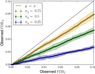
The two null hypotheses, and , gave different proportions of true null hypotheses among the discoveries. Here, we plotted the mean and SD of the Observed FDRA as a function of Observed FDRI over randomized simulations with different absent protein fractions, . The two Observed FDRs do not agree and for lower values of , that is, higher fractions of present proteins, this effect becomes more apparent.
3.2. A decoy model captures the number of incorrect protein inferences
We subsequently turned our attention to how well one can estimate the FDRI using a decoy model. Here, we simulated decoy peptide inferences under the assumptions of target–decoy analysis, that is, incorrect peptides have an equal probability of being a target as decoy peptide (see Section 1.2) 30. First, we plotted the fraction of proteins with incorrect best scoring peptide inference as a function of the classical decoy–target ratio, that is, the number of decoy proteins divided by the number of target proteins taken from the classical target–decoy protein list (Fig. 2).
Figure 2.
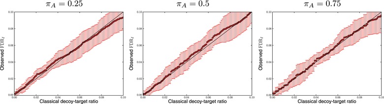
The number of proteins not supported by the best scoring peptide inference can be estimated by a decoy model. Here, we plotted the reported fraction of proteins with incorrect best scoring peptide inference as a function of the classical decoy–target ratio, for ten randomized simulations for three different values of the absent protein fraction, , and 20 000 peptide inferences. The classical decoy–target ratio accurately matches the fraction of proteins with incorrect best scoring peptide inference.
The classical decoy–target ratio serves as a way to capture the fraction of proteins with incorrect best scoring peptide inference. This makes sense as decoy proteins are models of incorrect inferences, an idea that holds up for PSMs, peptides, and proteins.
This approximation holds well as long as the set of peptide inferences belonging to present proteins is not sampled too deep. For long lists of peptide inferences (typically in our simulations), the probability of producing incorrect peptide matches belonging to proteins whose best scoring peptide inference is correct has to be taken into account 13. This effect causes the number of decoy proteins to be an overestimation of the number of incorrect proteins. One way to account for this effect is using the picked decoy–target ratio 17, that is, the number of decoy proteins divided by the number of target proteins taken from the picked target–decoy protein list (Fig. 3). We can hence say that the FDR of a list made using is approximately equal to the picked decoy–target ratio obtained at the threshold,
Figure 3.

For high coverage of the present peptide set, the picked target–decoy strategy should be used instead of the classical target–decoy strategy for an accurate estimation of the fraction of proteins with incorrect best scoring peptide inference. Here, for ten randomized simulations, we plotted the reported fraction of proteins with incorrect best scoring peptide inference as a function of (a) the classical decoy–target ratio and (b) the picked decoy–target ratio, for the same simulations of 80 000 peptide inferences and absent protein fraction, . The classical decoy–target ratio is no longer a good estimator for the fraction of proteins with incorrect best scoring peptide inference, and the picked decoy–target ratio should be used instead.
3.3. To estimate the number of absent proteins above threshold, we need an estimate of the global fraction of absent proteins
Next, we investigated the relationship between the proportion of absent proteins and the classical decoy–target ratio. From our simulated data, we calculated the proportion of absent proteins for a given protein list. We plotted the absence ratio as a function of the classical decoy–target ratio (Fig. 4).
Figure 4.
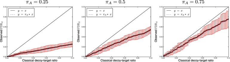
The protein absence ratio can be estimated by the classical decoy–target ratio, as long as we compensate for the absent protein fraction . We plotted the reported fraction of absent proteins as a function of the classical decoy–target ratio (red), together with a line (solid, black) and (dashed, blue) for ten randomized simulations with 20 000 peptide inferences. The protein absence ratio roughly corresponds to the classical decoy–target ratio times the absent protein fraction.
By multiplying the decoy–target ratio by the absent protein fraction, , the absence ratio can be estimated accurately. The absent protein fraction corrects for present proteins being inferred even though none of its peptides are actually correctly inferred. We can hence say that using the classical target–decoy protein list,
Without the correction, FDRA is overestimated by the classical decoy–target ratio. Therefore, the classical decoy–target ratio can be considered a conservative estimate of FDRA.
Note that using a picked target–decoy strategy would not give the same relation between its decoy–target ratio and FDRA. This is a consequence of correct target proteins more often eliminating their corresponding decoy protein than vice versa, which breaks the symmetry between target proteins with incorrect peptide matches and decoy proteins. Multiplying the picked decoy–target ratio by would in fact underestimate the fraction of absent proteins and should therefore be refrained from.
4. Discussion
Most practitioners of shotgun proteomics are interested in the lists of proteins, and a large fraction of all MS studies chooses to report a number of protein discoveries. A prerequisite for reporting error rates is a definition of what is meant with a false discovery, that is, a null hypothesis. It is important that MS‐based proteomics studies do not just report FDRs of their findings, but also which null hypothesis was used.
The FDR of a list of inferences is married to the specific question such a list answers. Here, we have demonstrated that the number of false discoveries made when inferring a list of proteins is dramatically different for two such null hypotheses, “false discoveries are proteins with incorrect best scoring peptide inference,” , and “false discoveries are absent proteins,” . Specifically, a researcher erroneously interpreting an FDR estimate generated under the null hypothesis , as the FDR estimated using the null hypothesis could end up with many more rejected null hypotheses than expected.
The null hypothesis, , that regards the absence of the protein and does not primarily include notions of peptides seems attractive for typical shotgun proteomics experiments. However, it should be noted that the approximation of the using a decoy model involves the absent protein fraction, , which is usually unknown. Estimation of is not trivial due to the indistinguishability of present proteins for which no peptides are detected and absent proteins. Currently, we have no good methods for estimating other than very conservative upper boundaries, such as the difference in the number of target and decoy proteins containing a spectrum match divided by the number of proteins in the target database.
The null hypothesis, , that regards the correctness of the best scoring peptide inference for a protein does not contain such an unknown parameter. However, it gives a somewhat unsatisfactory answer to what the sample actually contains. Furthermore, we cannot use mixtures of known protein content to verify its FDR estimates, nor can we verify its estimates on mixtures of unknown content by further experiments.
Here, we have shown that simulated data from a digestion and matching experiment can be used as a first check to assess the accuracy of FDR estimates. Given a well‐defined null hypothesis, one can simulate data in which the validity of the null hypothesis is known for each inference. Simulations thus provide a quick way to identify inaccurate estimates. One should, however, stay aware of the limitations imposed by the assumptions made. For instance, our simulation used a simplistic score distribution, and also does not try to mimic the effects of the difference in concentration of proteins. Furthermore, our sampling is done without replacement, which is a better model for low than high coverage situations.
One could think of many other questions regarding lists of proteins. Here are some examples: “Which proteins are inferred where all its protein‐specific peptides at a specific peptide‐level FDR are correctly matched?” “Which proteins contain more than N correctly inferred peptides that I can use for subsequent quantification?” “Which inferred proteins are present in different quantities in sample A and B?” “Which proteins are correctly inferred and present in different quantities in sample A and B?” As there is such a plethora of possible questions and corresponding null hypotheses, we see that reasoning about protein‐level FDRs becomes even harder, if we do not clearly define what we mean when we use the term.
The fact that the FDR is connected to the question posed when assembling the investigated list implies that one cannot trivially carry over an FDR of one list of inferences to another list of inferences, even if the lists contain similar information. We have shown this here for protein lists and different null hypotheses, but this rule is much more general. We cannot, for example, report PSM‐level FDR as the error measure for lists of unique peptides 14 or proteins. Nor can we transfer an FDR of a list of proteins from one experiment to a concatenated list of protein inferences 25.
We deliberately used an inference procedure that does not take peptides shared between different proteins into account. Lists of protein inferences in which shared peptide information is used correspond to more complicated questions, as we would need to make a more thorough definition of what is meant with correct and incorrect proteins. For example, should a protein with a correct peptide inference that is shared with other proteins be considered correct or not?
Grouping proteins based on shared peptides is commonly done in current methods, and can complicate the issue of shared peptides even further. For example, one could define a protein group to be a false discovery if all its proteins are absent or incorrect, but this is quite uninformative as we do not know which of its proteins are actually present or correct. Alternatively, one could define a false discovery as a protein group in which one of the proteins is absent or incorrect, but this would normally be too conservative. More fundamentally, such procedures force us to define the entities to which the null hypothesis applies to after we have seen data, that is, the protein groups are constructed after we inferred peptides from spectra 21.
Returning to the question of how one should talk about protein‐level FDRs, we think that one should separate the discussion about which null hypotheses are meaningful from the question of how accurate the FDR estimates are. Here, we have listed two null hypotheses that are meaningful, provided they are used in the right context, and can be accurately estimated. We highly encourage developers and users of protein inference methods to explicitly state their employed null hypothesis and, furthermore, to verify protein‐level FDR estimates with simulated data for a variety of common scenarios. We feel that these two simple steps will help to improve the field's understanding of protein‐level FDRs, as well as its confidence in them.
The authors have declared no conflict of interest.
Acknowledgements
The authors would like to thank Professor William Stafford Noble, University of Washington, for valuable comments on an early version of the manuscript.
Colour online: See the article online to view Figs. 1–4 in colour.
Footnotes
Note that, contrary to the prevalent nomenclature, we employ the term discovery instead of positive to indicate significant features, for example, false discovery instead of false‐positive. We feel that this emphasizes its relation to the FDR as opposed to creating a confounding connection to the false‐positive rate.
5 References
- 1. Sorić, B. , Statistical “discoveries” and effect‐size estimation. J. Am. Stat. Assoc. 1989, 84, 608–610. [Google Scholar]
- 2. Benjamini, Y. , Hochberg, Y. , Controlling the false discovery rate: a practical and powerful approach to multiple testing. J. R. Stat. Soc. 1995, 289–300. [Google Scholar]
- 3. Storey, J. D. , Tibshirani, R. , Statistical significance for genomewide studies. Proc. Natl. Acad. Sci. 2003, 100, 9440–9445. [DOI] [PMC free article] [PubMed] [Google Scholar]
- 4. Fenyö, D. , Beavis, R. C. , A method for assessing the statistical significance of mass spectrometry‐based protein identifications using general scoring schemes. Anal. Chem. 2003, 75, 768–774. [DOI] [PubMed] [Google Scholar]
- 5. Kim, S. , Gupta, N. , Pevzner, P. A. , Spectral probabilities and generating functions of tandem mass spectra: a strike against decoy databases. J. Proteome Res. 2008, 7, 3354–3363. [DOI] [PMC free article] [PubMed] [Google Scholar]
- 6. Keich, U. , Noble, W. S. , On the importance of well‐calibrated scores for identifying shotgun proteomics spectra. J. Proteome Res. 2014, 14, 1147–1160. [DOI] [PMC free article] [PubMed] [Google Scholar]
- 7. Nesvizhskii, A. I. , Aebersold, R. , Interpretation of shotgun proteomic data the protein inference problem. Mol. Cell. Proteomics 2005, 4, 1419–1440. [DOI] [PubMed] [Google Scholar]
- 8. Zhang, B. , Chambers, M. C. , Tabb, D. L. , Proteomic parsimony through bipartite graph analysis improves accuracy and transparency. J. Proteome Res. 2007, 6, 3549–3557. [DOI] [PMC free article] [PubMed] [Google Scholar]
- 9. Nesvizhskii, A. I. , Keller, A. , Kolker, E. , Aebersold, R. , A statistical model for identifying proteins by tandem mass spectrometry. Anal. Chem. 2003, 75, 4646–4658. [DOI] [PubMed] [Google Scholar]
- 10. Li, Y. F. , Arnold, R. J. , Li, Y. , Radivojac, P. et al., A Bayesian approach to protein inference problem in shotgun proteomics. J. Comput. Biol. 2009, 16, 1183–1193. [DOI] [PMC free article] [PubMed] [Google Scholar]
- 11. Serang, O. , MacCoss, M. J. , Noble, W. S. , Efficient marginalization to compute protein posterior probabilities from shotgun mass spectrometry data. J. Proteome Res. 2010, 9, 5346–5357. [DOI] [PMC free article] [PubMed] [Google Scholar]
- 12. Serang, O. , Noble, W. , A review of statistical methods for protein identification using tandem mass spectrometry. Stat. Interface 2012, 5, 3–20. [DOI] [PMC free article] [PubMed] [Google Scholar]
- 13. Reiter, L. , Claassen, M. , Schrimpf, S. P. , Jovanovic, M. et al., Protein identification false discovery rates for very large proteomics data sets generated by tandem mass spectrometry. Mol. Cell. Proteomics 2009, 8, 2405–2417. [DOI] [PMC free article] [PubMed] [Google Scholar]
- 14. Granholm, V. , Navarro, J. F. , Noble, W. S. , Käll, L. , Determining the calibration of confidence estimation procedures for unique peptides in shotgun proteomics. J. Proteomics 2013, 80, 123–131. [DOI] [PMC free article] [PubMed] [Google Scholar]
- 15. Li, Y. F. , Radivojac, P. , Computational approaches to protein inference in shotgun proteomics. BMC Bioinform. 2012, 13, S4. [DOI] [PMC free article] [PubMed] [Google Scholar]
- 16. Wilhelm, M. , Schlegl, J. , Hahne, H. , Gholami, A. M. et al., Mass‐spectrometry‐based draft of the human proteome. Nature 2014, 509, 582–587. [DOI] [PubMed] [Google Scholar]
- 17. Savitski, M. M. , Wilhelm, M. , Hahne, H. , Kuster, B. , Bantscheff, M. , A scalable approach for protein false discovery rate estimation in large proteomic data sets. Mol. Cell. Proteomics 2015, 14, 2394–2404. [DOI] [PMC free article] [PubMed] [Google Scholar]
- 18. Gigerenzer, G. , The superego, the ego, and the id in statistical reasoning, in: Keren G. and Lewis C. (Eds.), A Handbook for Data Analysis in the Behavioral Sciences: Methodological Issues, Psychology Press, New York: 1993, pp. 311–339. [Google Scholar]
- 19. Storey, J. D. , The positive false discovery rate: a Bayesian interpretation and the q‐value. Ann. Stat. 2003, 2013–2035. [Google Scholar]
- 20. Berger, J. O. , Could Fisher, Jeffreys and Neyman have agreed on testing? Stat. Sci. 2003, 18, 1–32. [Google Scholar]
- 21. Serang, O. , Moruz, L. , Hoopmann, M. R. , Käll, L. , Recognizing uncertainty increases robustness and reproducibility of mass spectrometry‐based protein inferences. J. Proteome Res. 2012, 11, 5586–91. [DOI] [PMC free article] [PubMed] [Google Scholar]
- 22. Klimek, J. , Eddes, J. S. , Hohmann, L. , Jackson, J. et al., The standard protein mix database: a diverse data set to assist in the production of improved peptide and protein identification software tools. J. Proteome Res. 2007, 7, 96–103. [DOI] [PMC free article] [PubMed] [Google Scholar]
- 23. Granholm, V. , Noble, W. S. , Kall, L. , On using samples of known protein content to assess the statistical calibration of scores assigned to peptide‐spectrum matches in shotgun proteomics. J. Proteome Res. 2011, 10, 2671–2678. [DOI] [PMC free article] [PubMed] [Google Scholar]
- 24. Bielow, C. , Aiche, S. , Andreotti, S. , Reinert, K. , Mssimulator: Simulation of mass spectrometry data. J. Proteome Res. 2011, 10, 2922–2929. [DOI] [PubMed] [Google Scholar]
- 25. Serang, O. , Käll, L. , Solution to statistical challenges in proteomics is more statistics, not less. J. Proteome Res. 2015, 14, 4099–4103. [DOI] [PubMed] [Google Scholar]
- 26. Moore, R. E. , Young, M. K. , Lee, T. D. , Qscore: an algorithm for evaluating sequest database search results. J. Am. Soc. Mass Spectrom. 2002, 13, 378–386. [DOI] [PubMed] [Google Scholar]
- 27. Käll, L. , Storey, J. D. , MacCoss, M. J. , Noble, W. S. , Assigning significance to peptides identified by tandem mass spectrometry using decoy databases. J. Proteome Res. 2007, 7, 29–34. [DOI] [PubMed] [Google Scholar]
- 28. Elias, J. E. , Gygi, S. P. , Target–decoy search strategy for mass spectrometry‐based proteomics, in: Hubbard S. J. and Jones A. R. (Eds.), Proteome Bioinformatics, Springer, New York: 2010, pp. 55–71. [DOI] [PMC free article] [PubMed] [Google Scholar]
- 29. Hubbard, T. , Barker, D. , Birney, E. , Cameron, G. et al., The Ensembl genome database project. Nucleic Acids Res. 2002, 30, 38–41. [DOI] [PMC free article] [PubMed] [Google Scholar]
- 30. Peng, J. , Elias, J. E. , Thoreen, C. C. , Licklider, L. J. , Gygi, S. P. , Evaluation of multidimensional chromatography coupled with tandem mass spectrometry (LC/LC‐MS/MS) for large‐scale protein analysis: the yeast proteome. J. Proteome Res. 2003, 2, 43–50. [DOI] [PubMed] [Google Scholar]