

Summary
Meta-analysis has become a widely used tool to combine results from independent studies. The collected studies are homogeneous if they share a common underlying true effect size; otherwise, they are heterogeneous. A fixed-effect model is customarily used when the studies are deemed homogeneous, while a random-effects model is used for heterogeneous studies. Assessing heterogeneity in meta-analysis is critical for model selection and decision making. Ideally, if heterogeneity is present, it should permeate the entire collection of studies, instead of being limited to a small number of outlying studies. Outliers can have great impact on conventional measures of heterogeneity and the conclusions of a meta-analysis. However, no widely accepted guidelines exist for handling outliers. This article proposes several new heterogeneity measures. In the presence of outliers, the proposed measures are less affected than the conventional ones. The performance of the proposed and conventional heterogeneity measures are compared theoretically, by studying their asymptotic properties, and empirically, using simulations and case studies.
Keywords: Absolute deviation, Heterogeneity, I2 statistic, Meta-analysis, Outliers
1. Introduction
Meta-analysis is a statistical method for combining a collection of effect estimates from multiple separate studies (Higgins and Green, 2008), and it has been applied in a wide range of scientific areas (Hunter and Schmidt, 1996; Prospective Studies Collaboration, 2002). The collected studies are called homogeneous if they share a common underlying true effect size; otherwise, they are called heterogeneous. A fixed-effect model is customarily used for studies deemed to be homogeneous, while a random-effects model is used for heterogeneous studies (Borenstein et al., 2010; Riley et al., 2011). Assessing heterogeneity is thus a critical issue in meta-analysis because different models may lead to different estimates of overall effect size and different standard errors. Also, the perception of heterogeneity or homogeneity helps clinicians make important decisions, such as whether the collected studies are similar enough to integrate their results and whether a treatment is applicable to all patients (Ioannidis et al., 2007).
The classical statistic for testing between-study heterogeneity is Cochran’s χ2 test (Cochran, 1954), also known as the Q test (Whitehead and Whitehead, 1991). However, this test suffers from poor power when the number of collected studies is small, and it may detect clinically unimportant heterogeneity when many studies are pooled (Hardy and Thompson, 1998; Jackson, 2006). More importantly, since the Q statistic and estimators of between-study variance depend on either the number of collected studies or the scale of effect sizes, they cannot be used to compare degrees of heterogeneity between different meta-analyses. Accordingly, Higgins and Thompson (2002) proposed several measures to better describe heterogeneity. Among these, I2 measures the proportion of total variation between studies that is due to heterogeneity rather than within-study sampling error, and it has been popular in the meta-analysis literature. Higgins and Green (2008) empirically provided a rough guide to interpretation of I2: 0 ≤ I2 ≤ 0.4 indicates that heterogeneity might not be important; 0.3 ≤ I2 ≤ 0.6 may represent moderate heterogeneity; 0.5 ≤ I2 ≤ 0.9 may represent substantial heterogeneity; and 0.75 ≤ I2 ≤ 1 implies considerable heterogeneity. These ranges overlap because the importance of heterogeneity depends on several factors and strict thresholds can be misleading (Higgins and Green, 2008).
Ideally, if heterogeneity is present in a meta-analysis, it should permeate the entire collection of studies instead of being limited to a small number of outlying studies. With this in mind, we may classify meta-analyses into four groups: (i) all the collected studies are homogeneous; (ii) a few studies are outlying and the rest are homogeneous; (iii) heterogeneity permeates the entire collection of studies; and (iv) a few studies are outlying and heterogeneity permeates the remaining studies. Outlying studies can have great impact on conventional heterogeneity measures and on the conclusions of a meta-analysis. Several methods have been recently developed for outliers and influence diagnostics (Viechtbauer and Cheung, 2010; Gumedze and Jackson, 2011). However, no widely accepted guidelines exist for handling outliers in the statistical literature, including the area of meta-analysis. Hedges and Olkin (1985) specified two extreme positions about dealing with outlying studies: (i) data are “sacred”, and no study should ever be set aside for any reason; or (ii) data should be tested for outlying studies, and those failing to conform to the hypothesized model should be removed. Neither seems appropriate. Alternatively, if a small number of studies is influential, some researchers usually present sensitivity analyses with and without those studies. However, if the results of sensitivity analysis differ dramatically, clinicians may reach no consensus about which result to use to make decisions. Because of these problems caused by outliers, ideal heterogeneity measures are expected to be robust: they should be minimally affected by outliers and accurately describe heterogeneity.
This article introduces several new heterogeneity measures, which are designed to be less affected by outliers than conventional measures. The basic idea comes from least absolute deviations (LAD) regression, which is known to have significant robustness advantages over classical least squares (LS) regression (Portnoy and Koenker, 1997). Specifically, LS regression aims at minimizing the sum of squared errors , where xi represents predictors, yi is the response, and β contains the regression coefficients. LAD regression minimizes the sum of absolute errors . The impact of outliers is diminished by using absolute values in LAD regression, compared to using squared values in LS regression. In meta-analysis, the conventional Q statistic has the form , where the yi’s are the observed effect sizes, the wi’s are study-specific weights, and is the weighted average effect size. Analogously, we consider a new measure , which is expected to be more robust against outliers than the conventional Q. An estimate of the between-study variance can be obtained based on Qr. Also, since Qr depends on the number of collected studies, we further derive two statistics to quantify heterogeneity, which are counterparts of I2 and another statistic H also proposed by Higgins and Thompson (2002).
This article is organized as follows. Section 2 gives a brief review of conventional measures and discusses the dilemma of handling outliers in meta-analysis. Section 3 proposes several new heterogeneity measures designed to be robust to outliers. Section 4 uses theoretical properties to compare the proposed and conventional measures. Section 5 presents simulations to compare the various approaches empirically, and Section 6 applies the approaches to two actual meta-analyses. Section 7 provides a brief discussion.
2. The conventional methods
2.1 Measures of between-study heterogeneity
Suppose that a meta-analysis contains n independent studies. Let μi be the underlying true effect size, such as log odds ratio, in study i (i = 1, …, n). Typically, published studies report estimates of the effect sizes and their within-study variances, which we will call yi and . It is customary to assume that the yi’s are approximately normally distributed with mean μi and variance , respectively. Since the unknown can be estimated by , these data are commonly modeled as with treated as known. Also, we assume that the true μi’s are independently distributed as , where μ is the true overall mean effect size across studies and τ2 is the between-study variance. The collected n studies are defined to be homogeneous if their underlying true effect sizes are equal, that is, μi = μ for all i = 1, …, n, or equivalently τ2 = 0. On the other hand, the studies are heterogeneous if their underlying true effect sizes vary, that is, τ2 > 0.
To test the homogeneity of the yi’s (i.e., H0: τ2 = 0 vs. HA: τ2 > 0), the well-known Q statistic (Whitehead and Whitehead, 1991) is defined as
which follows a distribution under the null hypothesis. Here, is the reciprocal of the within-study variance of yi, and is the pooled fixed-effect estimate of μ. Based on the Q statistic, DerSimonian and Laird (1986) introduced a method of moments estimate of the between-study variance,
Note that the Q statistic depends on the number of collected studies n and the estimate of between-study variance depends on the scale of effect sizes. Hence, neither Q nor can be used to compare degrees of heterogeneity between different meta-analyses. To allow such comparisons, Higgins and Thompson (2002) proposed the measures H and I2:
The H statistic is interpreted as the ratio of the standard deviation of the estimated overall effect size from a random-effects meta-analysis compared to the standard deviation from a fixed-effect meta-analysis; I2 describes the proportion of total variance between studies that is attributed to heterogeneity rather than sampling error. In practice, meta-analysts truncate H at 1 when H < 1 and truncate I2 at 0 when I2 < 0; therefore, H ⩾ 1 and I2 lies between 0 and 1. Since I2 is interpreted as a proportion, it is usually expressed as a percent. Both measures have been widely adopted in practice.
2.2 Outlier detection
As in many other statistical applications, outliers frequently appear in meta-analysis. Outliers may arise from at least three sources:
The quality of collected studies and systematic review. The published results (yi, ) in a clinical study could be outlying due to errors in the process of recording, analyzing, or reporting data. Also, the populations in certain clinical studies may not meet the systematic review’s inclusion criteria; hence, such studies may be outlying compared to most other collected studies.
A heavy-tailed distribution of study-specific underlying effect sizes. Conventionally, at the between-study level, the study-specific underlying effect sizes μi are assumed to have a normal distribution. However, the true distribution of the μi’s may greatly depart from the normality assumption and have heavy tails, such as the t-distribution with small degrees of freedom.
Small sample sizes in certain studies. The true within-study variances could be poorly estimated by the sample variances if the sample sizes are small. In some situations, effect sizes in small studies may be more informative than large studies due to “small study effects” (Nüesch et al., 2010); if their true within-study variances are seriously underestimated, then small studies could be outlying.
Hedges and Olkin (1985) and Viechtbauer and Cheung (2010) introduced outlier detection methods for fixed-effect and random-effects meta-analyses, respectively. Both methods use a “leave-one-study-out” technique so that a potential outlier could have little influence on the residuals of interest. Specifically, the residual of study i is calculated as . Here, is the estimated overall effect size using the data without study i; that is, under the fixed-effect setting, and under the random-effects setting, where can be the DerSimonian and Laird estimate using the data without study i. The variance of ei is estimated as and under the fixed-effect and random-effects settings, respectively. The standardized residuals are expected to follow the standard normal distribution and studies with εi’s greater than 3 in absolute magnitude are customarily considered outliers.
Outliers may be masked if the above approaches are used in an inappropriate setting. For example, Figures 3(b) and 3(d) in Section 6 show standardized residuals of two actual meta-analyses; different outlier detection methods identify different outliers. Hence, one must assess the heterogeneity of collected studies to correctly apply the foregoing approaches to detect outliers. However, outliers may cause heterogeneity to be overestimated and thus affect procedures to detect them. Additionally, even if outliers are identified, there is no consensus in the statistical literature on what to do about them unless these studies are evidently erroneous (Barnett and Lewis, 1994). To avoid the dilemmas of detecting and handling outliers, we propose robust measures to assess heterogeneity.
Figure 3.
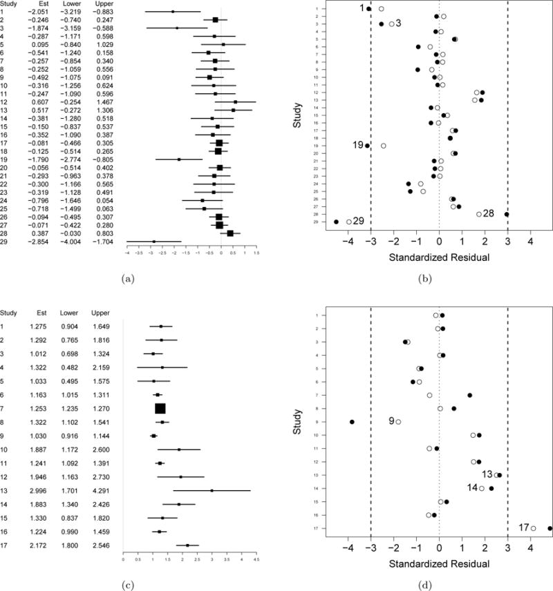
Forest plots and standardized residual plots of two actual meta-analyses. The upper panels show the meta-analysis conducted by Ismail et al. (2012); the lower panels show that conducted by Haentjens et al. (2010). In (a) and (c), the columns “Lower” and “Upper” are the lower and upper bounds of 95% CIs of the effect sizes within each study. In (b) and (d), the filled dots represent standardized residuals obtained under the fixed-effect setting; the unfilled dots represent those obtained under the random-effects setting.
3. The proposed alternative heterogeneity measures
3.1 Heterogeneity measures based on absolute deviations and weighted average
In linear regression, it is well-known that least absolute deviations regression is more robust to outliers than classical least squares regression (Portnoy and Koenker, 1997). The former method minimizes and the latter minimizes , where xi and yi are predictors and response respectively and β contains the regression coefficients. In the context of meta-analysis, the conventional Q statistic is analogous to least squares regression, because Q is a weighted sum of squared deviations. To reduce the impact of outlying studies, we propose a new measure Qr which is analogous to least absolute deviations regression. This measure is the weighted sum of absolute deviations, and is defined as
For random-effects meta-analysis, , where .
DerSimonian and Laird (1986) derived an estimate of the between-study variance τ2 based on the Q statistic by the method of moments, i.e., equating the observed Q with its expectation. We can similarly obtain a new estimate of τ2, denoted as , from the proposed Qr statistic. Specifically, is the solution to the following equation in τ2:
| (1) |
If this equation has no nonnegative solution, set . Note that the right-hand side of Equation (1) is monotone increasing in τ2, so the solution is unique.
The Qr statistic, like Q, is dependent on the number of studies; , like , is dependent on the scale of effect sizes. Following the approach of Higgins and Thompson (2002), we tentatively assume that all studies share a common within-study variance σ2 and explore heterogeneity measures that are independent of both the number of studies and the scale of effect sizes, so that they can be used to compare degrees of heterogeneity between meta-analyses. Suppose the target heterogeneity measure can be written as f(μ,τ2,σ2,n), which is a function of the true overall mean effect size μ, the between-study variance τ2, the within-study variance σ2, and the number of studies n. Higgins and Thompson (2002) suggested that this measure should satisfy the following three criteria:
(Dependence on the magnitude of heterogeneity) f(μ, τ′2, σ2,n) > f(μ, τ2, σ2, n) for any τ′2 > τ2. This criterion is self-evident.
(Scale invariance) f(a + bμ,b2τ2,b2σ2,n) = f(μ,τ2,σ2,n) for any constants a and b. This criterion “standardizes” comparisons between meta-analyses using different scales of measurement and different types of outcome data.
(Size invariance) f(μ,τ2,σ2,n′) = f(μ,τ2,σ2,n) for any positive integers n and n′. This criterion indicates that the number of studies collected in meta-analysis does not systematically affect the magnitude of the heterogeneity measure.
Monotone increasing functions of ρ = τ2/σ2 can be easily shown to satisfy these three criteria. Plugging wi = 1/σ2 into Equation (1), we have . This implies that
is a candidate measure. Further, considering ρ/(ρ + 1) = τ2/(τ2 + σ2), commonly called the intraclass correlation, Equation (1) yields another candidate:
In practice, Hr would be truncated at 1 when Hr < 1 and would be truncated at 0 when . These two measures, and , are analogous to and have the same interpretations as H2 and I2, respectively. Higgins and Thompson (2002) also introduced a so-called R2 statistic; since it has interpretation and performance similar to H2, we do not present a version of R2 based on the new Qr statistic.
Since standard deviations are used more frequently in clinical practice, Higgins and Thompson (2002) suggested reporting H, instead of H2, for meta-analyses. For the proposed measures, we also recommend reporting Hr rather than . However, we suggest presenting I2 and instead of their square roots because their interpretation of “proportion of variance explained” is widely familiar to clinicians. Hr = 1 or implies perfect homogeneity. Also, since the expressions for Hr and only involve Qr and n but not within-study variances, these two measures can be easily generalized to a situation where the within-study variances vary across studies.
3.2 Heterogeneity measures based on absolute deviations and weighted median
The proposed Qr statistic uses the weighted average to estimate overall effect size under the null hypothesis; it may be sensitive to potential outliers. To derive an even more robust heterogeneity measure, we may replace the weighted average with the weighted median , which is defined as the solution to the following equation in θ:
| (2) |
where is the indicator function. This weighted median leads to a new test statistic, . Note that the solution to Equation (2) may be not unique; to avoid this problem, we will approximate the indicator function by a monotone increasing smooth function (Horowitz, 1998). Section 3.3 introduces the details.
The expectation of Qm may not be explicitly calculated because the distribution of weighted median of finite samples is unclear. By the theory of M-estimation (Huber and Ronchetti, 2009), the weighted median is a -consistent estimator of the true overall effect size μ. Suppose that the weights wi have finite first-order moment, then it can be shown that
Therefore, when the number of collected studies n is large, . By equating the Qm statistic to its approximated expectation, a new estimator of between-study variance can be derived as the solution to in τ2. If all the within-study variances are further assumed to be equal to a common value σ2 as in Section 3.1, . Based on Qm, the counterparts of and —which assess (σ2 + τ2)/σ2 and τ2/(σ2 + τ2) respectively—are defined as
Note that many meta-analyses only collect a small number of studies; however, the derivation of , , and assumes a large n. The finite-sample performance of these heterogeneity measures will be studied using simulations.
3.3 Calculation of p-values and confidence intervals
Due to the difficulty caused by summing the absolute values of correlated random variables in the expression of Qr and the intractable distribution of weighted median in Qm, it is not feasible to explicitly derive the probability and cumulative density functions for the proposed statistics. Instead, resampling method can be used to calculate p-values and 95% confidence intervals (CIs). Since the weighted median in Qm is discontinuous and may be not unique due to the indicator function in Equation (2), we apply the approach in Horowitz (1998) to approximate the indicator function by a smooth function J(t) in the following simulations and case studies. For example, J(t) can be the scaled expit function , where ε is a pre-specified small constant. We use ε = 10−4; various choices of ε are shown to produce stable results in Web Appendix A.
Parametric resampling can be used to calculate a p-value for Qr; similar procedures can also be used for Q and Qm. First, estimate the overall effect size under H0: τ2 = 0 (i.e., the fixed-effect setting) and calculate the Qr statistic based on the original data. Second, draw n samples under H0, , and repeat this for B (say 10,000) iterations. Here, the weighted average is used to estimate μ because it is unbiased and may have smaller variance than the weighted median under the null hypothesis. Third, based on the B sets of bootstrap samples, calculate the Qr statistic as for b = 1, …, B. Finally, the p-value is calculated as . Here, 1 is added to both numerator and denominator to avoid calculating P = 0. To derive 95% CIs for the various heterogeneity measures, the nonparametric bootstrap can be used by taking samples of size n with replacement from the original data and calculating 2.5% and 97.5% quantiles for each of the measures over the bootstrap samples.
4. The relationship between I2, , and
4.1 When the number of studies is fixed
Since and are designed to be robust compared to the conventional I2, they are expected to be smaller than I2 in the presence of outliers. Applying the Cauchy-Schwarz Inequality, , and the equality holds if and only if each equals a common value for all studies, in which case outliers are unlikely to appear. The foregoing inequality further implies and . Therefore, the proposed Hr and are not always smaller than H and I2, respectively; may be greater than I2 by up to (1−2/π)(1−I2). Web Appendix B provides artificial meta-analyses to illustrate how the proposed measures may have better interpretations even when no outliers are present; and are larger than I2 in those examples. As is based on the intractable weighted median, determining its relationship with I2 and is not feasible in finite samples except by simulations. Alternatively, the asymptotic values of the three measures can be derived as n → ∞; Section 4.2 considers this case.
4.2 When the number of studies becomes large
This section focuses on the asymptotic properties of the three heterogeneity measures as the number of collected studies n → ∞. Denote as convergence in probability, and let Φ(·) be the cumulative distribution function of the standard normal distribution. We have the following two propositions if no outliers are present.
Proposition 1
Under the fixed-effect setting, the observed effect sizes are . Assume that the weights are independent and identically distributed with finite positive mean, and independent of the yi’s. Then I2, and converge to 0 in probability as n → ∞.
Proposition 2
Assume that all studies share a common within-study variance σ2. Under the random-effects setting, the observed effect sizes are yi ~ N(μi, σ2) and μi ~ N(μ, τ2); hence, the true proportion of total variation between studies due to heterogeneity is . Then I2, I2, and converge to the true in probability as n → ∞.
Propositions 1 and 2 show that, for either homogeneous or heterogeneous studies, all three heterogeneity measures converge to the true value and correctly indicate homogeneity or heterogeneity. Proposition 1 does not require that the n studies have a common within-study variance; Proposition 2 makes this assumption to facilitate definition of the true . The following proposition compares the three measures when the collection of studies is contaminated by a certain proportion of outlying studies.
Proposition 3
Assume that all studies share a common within-study variance σ2. The observed effect sizes are yi ~ N(μi, σ2). The meta-analysis is supposed to focus on a certain population of interest, and in this population, the study-specific underlying effect sizes are μi ~ N(μ, τ2); therefore, the true proportion of total variation between studies in this population that is due to heterogeneity is . However, 100η percent of the n studies are mistakenly included, having been conducted on inappropriate populations; their study-specific underlying effect sizes are μi ~ N(μ + C, τ2), where C is a constant, representing the discrepancy of outliers. Then, as n → ∞,
Here, h(·, ·; η, ) is a function depending on η and defined as
also, r1 = (1 − η)C/σ, r2 = ηC/σ, s2 = C/σ − s1, and s1 is the solution to
Web Appendix C gives proofs of the three propositions. Proposition 3 suggests that all the three heterogeneity measures are affected by outlying studies, though to different degrees. Specifically, their asymptotic values are determined by three factors: the true proportion of total variation between studies that is due to heterogeneity , the proportion of outliers η, and the ratio of the discrepancy of the outliers C compared to the within-study standard deviation σ, that is, R = C/σ. Outliers are usually present in small quantities, so the proportion of outliers η is usually not large. Also, an observation is customarily considered an outlier if the distance to the overall mean is greater than three times the standard deviation σ; therefore, the ratio R is usually greater than 3.
Figure 1 compares the asymptotic values of the three heterogeneity measures derived in Proposition 3. The upper panels show the setting of true homogeneity ( ) and the lower panels show the setting of true heterogeneity ( ). Under each setting, the proportion of outliers is 1%, 5%, or 10%. Clearly, all the panels present a common trend: the three heterogeneity measures increase as R increases. When η is 1%, and are much less affected by outliers than I2, indicating the robustness of the proposed measures. Also, is a bit smaller than . As η increases, the difference between I2 and becomes smaller, while the difference between and becomes larger though it is never substantial. This implies that is the most robust measure when a meta-analysis is contaminated by a large proportion of outliers.
Figure 1.
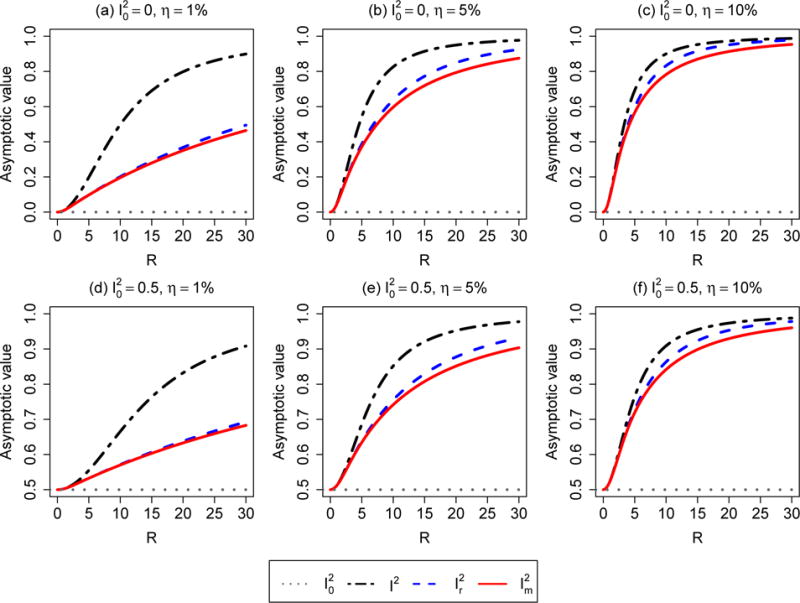
The asymptotic values of I2, , and as n → ∞. The horizontal axis represents the ratio (R) of discrepancy of outliers (C) compared to within-study standard deviation (σ), that is, R = C/σ. The true proportion of total variation between studies that is due to heterogeneity is 0 (homogeneity, top row) or 0.5 (heterogeneity, bottom row). The proportion of outlying studies η varies from 1% (left panels) to 10% (right panels).
5. Simulations
Simulations were conducted to investigate the finite-sample performance of the various approaches to assessing heterogeneity. Without loss of generality, the true overall mean effect size was fixed as μ = 0. The number of studies in these simulated meta-analyses was set to n = 10 or 30, and the between-study variance was τ2 = 0 (homogeneity) or 1 (heterogeneity). Under the homogeneity setting, the within-study standard errors si were sampled from U(0.5, 1); under the heterogeneity setting, we sampled si’s from U(smin, smax), where (smin, smax) = (0.5, 1), (1, 2), or (2, 5) to represent different proportions of total variation between studies that is due to heterogeneity. The observed effect sizes were drawn from , where μi’s are study-specific underlying effect sizes. Regarding the μi, we considered the following two different scenarios to produce outliers.
(Contamination) The μi’s are normally distributed, μi ~ N(μ, τ2); however, m out of the n studies were contaminated by a certain outlying discrepancy, as in Proposition 3. We set m = 0, 1, 2, and 3, and five outlier patterns were considered: the m studies were created as outliers by artificially adding C, (C, C), (C, − C), (C, C, C), or (C, C, −C) to the original effect sizes for m = 1, 2, 2, 3, and 3 respectively. The discrepancy of outliers was set to .
(Heavy tail) The μi’s are drawn from a heavy-tailed distribution. We considered a location-scale transformed t distribution with degrees of freedom df = 3, 5, and 10; that is, , where zi ~ tdf. Note that the between-study variance τ2 = Var[μi] = 1 in this scenario, so the generated studies are heterogeneous. Also, as degrees of freedom increases, the distribution of μi’s converges to the normal distribution and outliers are less likely.
Table 1 presents some results for n = 30, including statistical sizes (type I error rates) and powers of the statistics Q, Qr, and Qm for testing H0: τ2 = 0 vs. HA: τ2 > 0, and the root mean squared errors (RMSEs) and coverage probabilities of 95% CIs of , , and . Web Appendix D contains complete simulation results. When the studies are homogeneous, each of the three test statistics controls type I error rate well if no outliers are present. Also, the RMSEs of the three estimators of τ2 are close and their coverage probabilities are fairly high. However, when outliers appear, the type I error rate of Q inflates dramatically compared to Qr and Qm. The RMSE of becomes larger than those of and ; also, the coverage probability of is lower, especially when m = 3. As the number of outliers increases, the weighted-median-based has smaller RMSE and its 95% CI has higher coverage probability than the weighted-mean-based .
Table 1.
Some simulation results for meta-analyses containing 30 studies.
| Outlier pattern | Size/power†
|
RMSE |
CP (%) |
|||||||||||
|---|---|---|---|---|---|---|---|---|---|---|---|---|---|---|
| Q‡ | Qr | Qm |
|
|
|
|
|
|
||||||
| Scenario I (contamination) with τ2 = 0 (homogeneity) and si ~ U(0.5, 1): | ||||||||||||||
| No outliers | 0.05 (0.06) | 0.05 | 0.05 | 0.10 | 0.12 | 0.10 | 98 | 99 | 99 | |||||
| C | 0.55 (0.55) | 0.27 | 0.25 | 0.37 | 0.24 | 0.20 | 97 | 97 | 98 | |||||
| (C, C) | 0.89 (0.89) | 0.66 | 0.60 | 0.63 | 0.42 | 0.35 | 88 | 90 | 94 | |||||
| (C, −C) | 0.92 (0.92) | 0.61 | 0.61 | 0.68 | 0.40 | 0.36 | 89 | 90 | 94 | |||||
| (C, C, C) | 0.98 (0.98) | 0.90 | 0.87 | 0.88 | 0.64 | 0.53 | 65 | 74 | 83 | |||||
| (C, C, −C) | 0.99 (0.98) | 0.89 | 0.88 | 0.99 | 0.61 | 0.55 | 64 | 73 | 83 | |||||
|
| ||||||||||||||
| Scenario I (contamination) with τ2 = 1 (heterogeneity) and si ~ U(0.5, 1): | ||||||||||||||
| No outliers | 0.98 (0.99) | 0.98 | 0.98 | 0.40 | 0.43 | 0.41 | 88 | 93 | 91 | |||||
| C | 1.00 (1.00) | 1.00 | 1.00 | 0.84 | 0.63 | 0.55 | 97 | 97 | 98 | |||||
| (C, C) | 1.00 (1.00) | 1.00 | 1.00 | 1.37 | 1.00 | 0.85 | 93 | 94 | 96 | |||||
| (C, −C) | 1.00 (1.00) | 1.00 | 1.00 | 1.45 | 0.97 | 0.85 | 93 | 94 | 96 | |||||
| (C, C, C) | 1.00 (1.00) | 1.00 | 1.00 | 1.86 | 1.44 | 1.22 | 76 | 83 | 90 | |||||
| (C, C, −C) | 1.00 (1.00) | 1.00 | 1.00 | 2.05 | 1.40 | 1.25 | 77 | 84 | 91 | |||||
|
| ||||||||||||||
| Scenario I (contamination) with τ2 = 1 (heterogeneity) and si ~ U(1, 2): | ||||||||||||||
| No outliers | 0.48 (0.49) | 0.42 | 0.43 | 0.74 | 0.81 | 0.75 | 89 | 93 | 91 | |||||
| C | 0.89 (0.89) | 0.78 | 0.77 | 1.97 | 1.36 | 1.17 | 98 | 97 | 98 | |||||
| (C, C) | 0.99 (0.99) | 0.94 | 0.94 | 3.33 | 2.29 | 1.93 | 91 | 92 | 96 | |||||
| (C, −C) | 0.99 (0.99) | 0.94 | 0.94 | 3.50 | 2.17 | 1.93 | 91 | 92 | 96 | |||||
| (C, C, C) | 1.00 (1.00) | 0.99 | 0.99 | 4.60 | 3.41 | 2.85 | 70 | 80 | 88 | |||||
| (C, C, −C) | 1.00 (1.00) | 0.99 | 0.99 | 5.03 | 3.24 | 2.90 | 71 | 81 | 88 | |||||
|
| ||||||||||||||
| Scenario II (heavy tail) with τ2 = 1 (heterogeneity) and si ~ U(0.5, 1): | ||||||||||||||
| df = 3 | 0.92 (0.92) | 0.89 | 0.88 | 1.45 | 0.59 | 0.56 | 72 | 79 | 73 | |||||
| df = 5 | 0.98 (0.98) | 0.95 | 0.95 | 0.55 | 0.45 | 0.45 | 84 | 90 | 86 | |||||
| df = 10 | 0.98 (0.98) | 0.97 | 0.97 | 0.43 | 0.43 | 0.42 | 88 | 93 | 90 | |||||
|
| ||||||||||||||
| Scenario II (heavy tail) with τ2 = 1 (heterogeneity) and si ~ U(1, 2): | ||||||||||||||
| df = 3 | 0.41 (0.40) | 0.35 | 0.35 | 1.53 | 0.88 | 0.82 | 83 | 90 | 87 | |||||
| df = 5 | 0.46 (0.46) | 0.40 | 0.40 | 0.82 | 0.82 | 0.77 | 88 | 93 | 90 | |||||
| df = 10 | 0.48 (0.49) | 0.42 | 0.42 | 0.76 | 0.82 | 0.77 | 88 | 94 | 90 | |||||
RMSE: root mean squared error; CP: coverage probability of 95% confidence interval.
Size (type I error rate) for homogeneous studies (τ2 = 0) and power for heterogeneous studies (τ2 > 0) at the significance level α = 0.05.
The sizes/powers outside the parentheses are produced by the resampling method; those inside the parentheses are obtained using Q’s theoretical distribution under the null hypothesis.
For heterogeneous studies, the conventional Q statistic is more powerful than Qr or Qm, but the differences are not large; this is expected because Q sacrifices type I error in the presence of outliers. In spite of this disadvantage of Qr and Qm, the proposed estimators of τ2 still perform better than the conventional in both Scenarios I and II.
Figure 2 compares the impact of a single outlier in Scenario I with m = 1 on the heterogeneity measures I2, , and . As expected, these heterogeneity measures generally increase due to the outlying study, so their changes are mostly greater than 0. However, for both homogeneous and heterogeneous studies, the changes of and are generally smaller than the changes of I2, indicating that the proposed measures are indeed less affected by outliers than the conventional I2.
Figure 2.
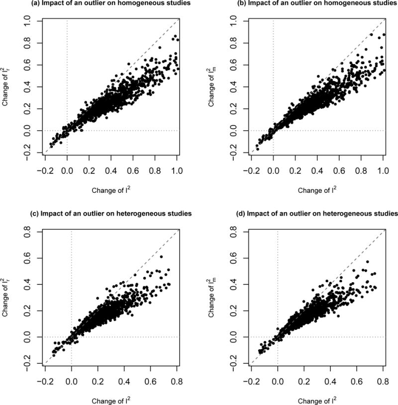
Scatter plots of the changes of and due to an outlier against the changes of I2. For the upper panels, τ2 = 0 (homogeneous studies) and si ~ U(0.5, 1); for the lower panels, τ2 = 1 (heterogeneous studies) and si ~ U(1, 2). The left panels compare with I2; the right panels compare with I2.
6. Two case studies
6.1 Homogeneous studies with outliers
Ismail et al. (2012) reported a meta-analysis consisting of 29 studies to evaluate the effect of aerobic exercise (AEx) on visceral adipose tissue (VAT) content/volume in overweight and obese adults, compared to control treatment. Figure 3(a) shows the forest plot with the observed effect sizes and their within-study 95% CIs; studies 1, 3, 19, and 29 seem to be outlying. If these four studies are removed, the remaining studies are much more homogeneous. Figure 3(b) presents the standardized residuals using both the fixed-effect and random-effects approaches described in Section 2.2. Studies 1, 19, and 29 have standardized residuals (under the fixed-effect setting) greater than 3 in absolute magnitude; hence, they may be considered outliers. We conducted sensitivity analysis by removing the following studies: (i) 1; (ii) 19; (iii) 29; (iv) 1 and 19; (v) 1 and 29; (vi) 19 and 29; and (vii) 1, 19, and 29.
Table 2 presents the results for the original meta-analysis and for alternate meta-analyses removing certain outlying studies. For the original meta-analysis, and , compared to I2 = 0.59. Also, and are smaller than . To test H0: τ2 = 0 vs. HA: τ2 > 0, the p-value of the Q statistic is smaller than 0.001, and those of the Qr and Qm statistics are 0.013 and 0.006, respectively. When study 29 is removed, the Q statistic is still significant (p-value = 0.008), while the p-values of the Qr and Qm statistics are larger than the commonly used significance level α = 0.05. After removing all three outlying studies, the p-values of the three test statistics are much larger than 0.05; also, and I2 = 0.11. Hence, the heterogeneity presented in the original meta-analysis is mainly caused by the few outliers. Note that and are still noticeably smaller than I2 after removing the three identified outliers. This may be because some studies other than studies 1, 19, and 29 are potentially outlying. Figure 3(b) shows that the absolute values of the standardized residuals of studies 3 and 28 are fairly close to 3. Although some outliers may not be clearly detected, and automatically reduce their impact without removing them.
Table 2.
Summary results for two actual meta-analyses.
| Removed studies |
p-value of
testing H0:
τ2 = 0 |
Estimated
τ (95% CI) |
Heterogeneity measure
(95% CI) |
||||||||||
|---|---|---|---|---|---|---|---|---|---|---|---|---|---|
| Q† | Qr | Qm |
|
|
|
I2 |
|
|
|||||
| Meta-analysis in Ismail et al. (2012): | |||||||||||||
| None (Original) | < 0.001 (< 0.001) | 0.013 | 0.006 | 0.39 (0, 0.62) | 0.29 (0, 0.58) | 0.30 (0, 0.56) | 0.59 (0, 0.76) | 0.44 (0, 0.73) | 0.45 (0, 0.72) | ||||
| 1 | < 0.001 (< 0.001) | 0.047 | 0.030 | 0.35 (0, 0.58) | 0.24 (0, 0.52) | 0.24 (0, 0.51) | 0.55 (0, 0.75) | 0.36 (0, 0.69) | 0.36 (0, 0.69) | ||||
| 19 | < 0.001 (< 0.001) | 0.048 | 0.031 | 0.34 (0, 0.58) | 0.24 (0, 0.52) | 0.24 (0, 0.51) | 0.54 (0, 0.75) | 0.36 (0, 0.69) | 0.36 (0, 0.68) | ||||
| 29 | 0.008 (0.007) | 0.100 | 0.070 | 0.28 (0, 0.46) | 0.21 (0, 0.44) | 0.21 (0, 0.43) | 0.44 (0, 0.66) | 0.29 (0, 0.63) | 0.30 (0, 0.62) | ||||
| 1 and 19 | 0.003 (0.004) | 0.154 | 0.121 | 0.29 (0, 0.54) | 0.18 (0, 0.45) | 0.18 (0, 0.44) | 0.47 (0, 0.73) | 0.25 (0, 0.64) | 0.24 (0, 0.63) | ||||
| 1 and 29 | 0.052 (0.052) | 0.272 | 0.223 | 0.22 (0, 0.40) | 0.14 (0, 0.37) | 0.13 (0, 0.36) | 0.33 (0, 0.60) | 0.16 (0, 0.56) | 0.15 (0, 0.55) | ||||
| 19 and 29 | 0.057 (0.057) | 0.278 | 0.232 | 0.21 (0, 0.40) | 0.13 (0, 0.38) | 0.13 (0, 0.37) | 0.32 (0, 0.60) | 0.15 (0, 0.56) | 0.14 (0, 0.55) | ||||
| 1, 19 and 29 | 0.302 (0.298) | 0.547 | 0.504 | 0.11 (0, 0.30) | 0 (0, 0.29) | 0 (0, 0.27) | 0.11 (0, 0.47) | 0 (0, 0.46) | 0 (0, 0.42) | ||||
|
| |||||||||||||
| Meta-analysis in Haentjens et al. (2010): | |||||||||||||
| None (Original) | < 0.001 (< 0.001) | < 0.001 | < 0.001 | 0.16 (0.02, 0.34) | 0.15 (0, 0.37) | 0.08 (0, 0.36) | 0.74 (0.15, 0.86) | 0.66 (0, 0.85) | 0.63 (0, 0.85) | ||||
| 9 | < 0.001 (< 0.001) | 0.006 | 0.006 | 0.16 (0, 0.37) | 0.13 (0, 0.42) | 0.06 (0, 0.37) | 0.68 (0, 0.84) | 0.56 (0, 0.83) | 0.52 (0, 0.81) | ||||
| 17 | 0.001 (0.001) | 0.013 | 0.015 | 0.11 (0, 0.23) | 0.11 (0, 0.27) | 0.05 (0, 0.27) | 0.60 (0, 0.76) | 0.52 (0, 0.77) | 0.47 (0, 0.76) | ||||
| 9 and 17 | 0.062 (0.059) | 0.156 | 0.144 | 0.09 (0, 0.24) | 0.07 (0, 0.27) | 0.02 (0, 0.25) | 0.39 (0, 0.65) | 0.28 (0, 0.67) | 0.23 (0, 0.65) | ||||
The p-values outside the parentheses are produced by the resampling method; the p-values inside the parentheses are calculated using Q’s theoretical distribution under the null hypothesis.
6.2 Heterogeneous studies with outliers
Haentjens et al. (2010) investigated the magnitude and duration of excess mortality after hip fracture among older men by performing a meta-analysis consisting of 17 studies. Figure 3(c) shows the forest plot with the observed effect sizes (log hazard ratios) and their 95% within-study CIs. The forest plot indicates that the collected studies tend to be heterogeneous. Despite this, we used both the fixed-effect and random-effects diagnostic procedure in Section 2.2 to detect potential outliers. Figure 3(d) shows the study-specific standardized residuals, indicating that study 17 is apparently outlying. Although study 9’s standardized residual is smaller than 2 in absolute magnitude when using the random-effects approach, its standardized residual under the fixed-effect setting is fairly large. To take all potential outliers into account, we conducted sensitivity analysis by removing the following studies: (i) 9; (ii) 17; and (iii) 9 and 17.
The results are in Table 2. For the original meta-analysis, the p-values of all the three test statistics are smaller than 0.001, rejecting the null hypothesis of homogeneity. Also, I2 = 0.74, and , indicating substantial heterogeneity. If study 9 is removed, the results seem to change little, implying that this study is not influential. If study 17 is removed, the p-values of the test statistics change noticeably; also, each of I2, , and is reduced by more than 0.10. The three heterogeneity measures are still fairly high (larger than or close to 0.5); therefore, meta-analysts may keep paying attention to the heterogeneity of the remaining studies.
7. Discussion
This paper proposed several alternative measures of heterogeneity in meta-analysis. Large-sample properties and finite-sample studies showed that the new measures are robust to outliers compared with conventional measures. Since outliers frequently appear in meta-analysis and may not simply be removed without sound evidence, the proposed robust measures can provide useful information describing heterogeneity. The robustness of the new approaches mainly arises from using the absolute deviations in the Qr and Qm statistics; Qr summarizes the deviations using the weighted average, and Qm summarizes the deviations using the weighted median. Note that the number of studies is assumed to be large in deriving , Hm, and . However, many meta-analyses may only collect a few studies (Davey et al., 2011); these three measures need to be used with caution for small meta-analyses.
When study-level covariates are collected in meta-analysis, meta-regression is widely applied to investigate whether study characteristics explain heterogeneity (Higgins and Thompson, 2004). To improve robustness to outliers, instead of performing least squares regression, researchers may consider least absolute deviations regression (Portnoy and Koenker, 1997), which is related to the heterogeneity measures proposed in this article.
Heterogeneity measures are customarily used to select a fixed-effect or random-effects model, but both models have limitations in certain situations. Some researchers believe that heterogeneity is to be expected in any meta-analysis because the collected studies were performed by different teams in different places using different methods (Higgins, 2008). Also, the fixed-effect model produces confidence intervals with poor coverage probability when the collected studies have different true effect sizes (Hedges and Vevea, 1998), so some researchers recommend routinely using the random-effects model to yield conservative results (Chalmers, 1991). However, the random-effects model is not always better than the fixed-effect model, especially in the presence of publication bias (Poole and Greenland, 1999; Henmi and Copas, 2010; Stanley and Doucouliagos, 2015). Besides robustly assessing heterogeneity, alternative approaches to robustly estimating overall effects size in the presence of outliers remain to be studied.
The R code for the proposed methods are organized in the package altmeta and available at http://cran.r-project.org/package=altmeta.
Supplementary Material
Acknowledgments
This research was supported in part by NIAID R21 AI103012 (HC, LL), NIDCR R03 DE024750 (HC), NLM R21 LM012197 (HC), and NIDDK U01 DK106786 (HC).
Footnotes
Supplementary Materials
Web Appendix A referenced in Section 3.3, Web Appendix B referenced in Section 4.1, Web Appendix C referenced in Section 4.2, and Web Appendix D referenced in Section 5 are available with this paper at the Biometrics website on Wiley Online Library.
References
- Barnett V, Lewis T. Outliers in Statistical Data. 3rd John Wiley & Sons; New York, NY: 1994. [Google Scholar]
- Borenstein M, Hedges LV, Higgins JPT, Rothstein HR. A basic introduction to fixed-effect and random-effects models for meta-analysis. Research Synthesis Methods. 2010;1:97–111. doi: 10.1002/jrsm.12. [DOI] [PubMed] [Google Scholar]
- Chalmers TC. Problems induced by meta-analyses. Statistics in Medicine. 1991;10:971–980. doi: 10.1002/sim.4780100618. [DOI] [PubMed] [Google Scholar]
- Cochran WG. The combination of estimates from different experiments. Biometrics. 1954;10:101–129. [Google Scholar]
- Davey J, Turner RM, Clarke MJ, Higgins JPT. Characteristics of meta-analyses and their component studies in the cochrane database of systematic reviews: a cross-sectional, descriptive analysis. BMC Medical Research Methodology. 2011;11:160. doi: 10.1186/1471-2288-11-160. [DOI] [PMC free article] [PubMed] [Google Scholar]
- DerSimonian R, Laird N. Meta-analysis in clinical trials. Controlled Clinical Trials. 1986;7:177–188. doi: 10.1016/0197-2456(86)90046-2. [DOI] [PubMed] [Google Scholar]
- Gumedze FN, Jackson D. A random effects variance shift model for detecting and accommodating outliers in meta-analysis. BMC Medical Research Methodology. 2011;11:19. doi: 10.1186/1471-2288-11-19. [DOI] [PMC free article] [PubMed] [Google Scholar]
- Haentjens P, Magaziner J, Colón-Emeric CS, Vanderschueren D, Milisen K, Velkeniers B, Boonen S. Meta-analysis: excess mortality after hip fracture among older women and men. Annals of Internal Medicine. 2010;152:380–390. doi: 10.1059/0003-4819-152-6-201003160-00008. [DOI] [PMC free article] [PubMed] [Google Scholar]
- Hardy RJ, Thompson SG. Detecting and describing heterogeneity in meta-analysis. Statistics in Medicine. 1998;17:841–856. doi: 10.1002/(sici)1097-0258(19980430)17:8<841::aid-sim781>3.0.co;2-d. [DOI] [PubMed] [Google Scholar]
- Hedges LV, Olkin I. Statistical Method for Meta-Analysis. Academic Press; Orlando, FL: 1985. [Google Scholar]
- Hedges LV, Vevea JL. Fixed- and random-effects models in meta-analysis. Psychological Methods. 1998;3:486–504. [Google Scholar]
- Henmi M, Copas JB. Confidence intervals for random effects meta-analysis and robustness to publication bias. Statistics in Medicine. 2010;29:2969–2983. doi: 10.1002/sim.4029. [DOI] [PubMed] [Google Scholar]
- Higgins JPT. Commentary: Heterogeneity in meta-analysis should be expected and appropriately quantified. International Journal of Epidemiology. 2008;37:1158–1160. doi: 10.1093/ije/dyn204. [DOI] [PubMed] [Google Scholar]
- Higgins JPT, Green S. Cochrane Handbook for Systematic Reviews of Interventions. John Wiley & Sons; Chichester, UK: 2008. [Google Scholar]
- Higgins JPT, Thompson SG. Quantifying heterogeneity in a meta-analysis. Statistics in Medicine. 2002;21:1539–1558. doi: 10.1002/sim.1186. [DOI] [PubMed] [Google Scholar]
- Higgins JPT, Thompson SG. Controlling the risk of spurious findings from meta-regression. Statistics in Medicine. 2004;23:1663–1682. doi: 10.1002/sim.1752. [DOI] [PubMed] [Google Scholar]
- Horowitz JL. Bootstrap methods for median regression models. Econometrica. 1998;66:1327–1351. [Google Scholar]
- Huber PJ, Ronchetti EM. Robust Statistics. 2nd John Wiley & Sons; Hoboken, NJ: 2009. [Google Scholar]
- Hunter JE, Schmidt FL. Cumulative research knowledge and social policy formulation: the critical role of meta-analysis. Psychology, Public Policy, and Law. 1996;2:324–347. [Google Scholar]
- Ioannidis JPA, Patsopoulos NA, Evangelou E. Uncertainty in heterogeneity estimates in meta-analyses. BMJ. 2007;335:914. doi: 10.1136/bmj.39343.408449.80. [DOI] [PMC free article] [PubMed] [Google Scholar]
- Ismail I, Keating SE, Baker MK, Johnson NA. A systematic review and meta-analysis of the effect of aerobic vs. resistance exercise training on visceral fat. Obesity Reviews. 2012;13:68–91. doi: 10.1111/j.1467-789X.2011.00931.x. [DOI] [PubMed] [Google Scholar]
- Jackson D. The power of the standard test for the presence of heterogeneity in meta-analysis. Statistics in Medicine. 2006;25:2688–2699. doi: 10.1002/sim.2481. [DOI] [PubMed] [Google Scholar]
- Nüesch E, Trelle S, Reichenbach S, Rutjes AWS, Tschannen B, Altman DG, Egger M, Jüni P. Small study effects in meta-analyses of osteoarthritis trials: meta-epidemiological study. BMJ. 2010;341:c3515. doi: 10.1136/bmj.c3515. [DOI] [PMC free article] [PubMed] [Google Scholar]
- Poole C, Greenland S. Random-effects meta-analyses are not always conservative. American Journal of Epidemiology. 1999;150:469–475. doi: 10.1093/oxfordjournals.aje.a010035. [DOI] [PubMed] [Google Scholar]
- Portnoy S, Koenker R. The gaussian hare and the laplacian tortoise: computability of squared-error versus absolute-error estimators (with discussion) Statistical Science. 1997;12:279–300. [Google Scholar]
- Prospective Studies Collaboration. Age-specific relevance of usual blood pressure to vascular mortality: a meta-analysis of individual data for one million adults in 61 prospective studies. The Lancet. 2002;360:1903–1913. doi: 10.1016/s0140-6736(02)11911-8. [DOI] [PubMed] [Google Scholar]
- Riley RD, Higgins JPT, Deeks JJ. Interpretation of random effects meta-analyses. BMJ. 2011;342:d549. doi: 10.1136/bmj.d549. [DOI] [PubMed] [Google Scholar]
- Stanley TD, Doucouliagos H. Neither fixed nor random: weighted least squares meta-analysis. Statistics in Medicine. 2015;34:2116–2127. doi: 10.1002/sim.6481. [DOI] [PubMed] [Google Scholar]
- Viechtbauer W, Cheung MWL. Outlier and influence diagnostics for meta-analysis. Research Synthesis Methods. 2010;1:112–125. doi: 10.1002/jrsm.11. [DOI] [PubMed] [Google Scholar]
- Whitehead A, Whitehead J. A general parametric approach to the meta-analysis of randomized clinical trials. Statistics in Medicine. 1991;10:1665–1677. doi: 10.1002/sim.4780101105. [DOI] [PubMed] [Google Scholar]
Associated Data
This section collects any data citations, data availability statements, or supplementary materials included in this article.