Multifractal Texture Estimation for Detection and Segmentation of Brain Tumors

Abstract

A stochastic model for characterizing tumor texture in brain magnetic resonance (MR) images is proposed. The efficacy of the model is demonstrated in patient-independent brain tumor texture feature extraction and tumor segmentation in magnetic resonance images (MRIs). Due to complex appearance in MRI, brain tumor texture is formulated using a multiresolution-fractal model known as multifractional Brownian motion (mBm). Detailed mathematical derivation for mBm model and corresponding novel algorithm to extract spatially varying multifractal features are proposed. A multifractal feature-based brain tumor segmentation method is developed next. To evaluate efficacy, tumor segmentation performance using proposed multifractal feature is compared with that using Gabor-like multiscale texton feature. Furthermore, novel patient-independent tumor segmentation scheme is proposed by extending the well-known AdaBoost algorithm. The modification of AdaBoost algorithm involves assigning weights to component classifiers based on their ability to classify difficult samples and confidence in such classification. Experimental results for 14 patients with over 300 MRIs show the efficacy of the proposed technique in automatic segmentation of tumors in brain MRIs. Finally, comparison with other state-of-the art brain tumor segmentation works with publicly available low-grade glioma BRATS2012 dataset show that our segmentation results are more consistent and on the average outperforms these methods for the patients where ground truth is made available.

I. Introduction

Varying intensity of tumors in brain magnetic resonance images (MRIs) makes the automatic segmentation of such tumors extremely challenging. Brain tumor segmentation using MRI has been an intense research area. Both feature-based [1]–[8] and atlas-based [9]–[11] techniques as well as their combinations [12] have been proposed for brain tumor segmentation. In [10], Warfield et al. combined elastic atlas registration with statistical classification to mask brain tissue from surrounding structures. Kaus et al. [11] proposed brain tumor segmentation using digital anatomic atlas and MR image intensity. However, the method requires manual selection of three or four example voxels for each tissue class for a patient. In [9], Prastawa et al. developed tumor segmentation and statistical classification of brain MR images using an atlas prior. There are few challenges associated with atlas-based segmentation. Atlas-based segmentation requires manual labeling of template MRI. In addition, the elastic registration of template MRI with distorted patient images due to pathological processes is nontrivial. It may pose further challenge in detecting tumor from postoperative patient MRI where the deformation may be more extensive. Such issues with atlas-based tumor segmentation can be mitigated by devising complementary techniques to aid tumor segmentation [13], [14]. In [13], Davatzikos et al. used systematic deformations due to tumor growth to match pre-operative images of the patient with that of the postoperative. In [14], Menze et al. proposed a generative probabilistic model for segmentation by augmenting atlas of healthy tissue priors with a latent atlas of tumor.

Among feature-based techniques, Lee et al. [2] proposed brain tumor segmentation using discriminative random field (DRF) method. In [2], Lee et al. exploited a set of multiscale image-based and alignment-based features for segmentation. However, the proposed framework does not allow training and testing the proposed models across different patients. Corso et al. [3] discussed conditional random field (CRF) based hybrid discriminative-generative model for segmentation and labeling of brain tumor tissues in MRI. The CRF model employs cascade of boosted discriminative classifier where each classifier uses a set of about one thousand features. Wels et al. [5] used intensity, intensity gradient, and Haar-like features in a Markov random field (MRF) method that combines probabilistic boosting trees and graph cuts for tumor segmentation. Overall, these methods of incorporating spatial dependencies in classification using DRF/CRF/MRF demand very careful tumor characterization for convergence.

Gering et al. [12] proposed a promising framework for brain tumor segmentation by recognizing deviation from normal tissue. However, the proposed technique in [12] depends on manual corrective action between iterations. Cobzas et al. [4] studied textons [15] and level set features with atlas-based priors to build statistical models for tissues. Such level set techniques are very sensitive to initialization and known to suffer from boundary leaking artifacts. In [8], Wang et al. proposed a parametric active contour model that facilitates brain tumor detection in MRI. The proposed model makes rather simplistic assumption that there is a single continuous region associated with tumor. Bauer et al. [16] exploited patient-specific initial probabilities with nonlocal features to capture context information. Bauer et al. used a standard classification forest (CF) as a discriminative multiclass classification model. The techniques in [16] combined random forest (RF) classification with hierarchical CRF regularization as an energy minimization scheme for tumor segmentation. In [17], Geremia et al. introduced a symmetry feature and RF classification for automated tumor segmentation. Recently, Hamamci and Unal [18] proposed a multimodal modified tumor-cut method for tumor and edema segmentation. The proposed method needs user interaction to draw maximum diameter of the tumor. Raviv et al. [19] presented a statistically driven level-set approach for segmentation of subject-specific MR scans. The technique is based on latent atlas approach, where common information from different MRI modalities is captured using spatial probability. However, this method also requires manual initialization of tumor seed and boundary for effective segmentation.

Among texture feature extraction techniques, fractal analysis has shown success in tumor segmentation [1], [6], [7]. In prior works [1], [20], we demonstrate effectiveness of fractal features in segmenting brain tumor tissue. Considering intricate pattern of tumor texture, regular fractal-based feature extraction techniques appear rather homogeneous. We argue that the complex texture pattern of brain tumor in MRI may be more amenable to multifractional Brownian motion (mBm) analysis [6], [7], [21]. In [21], we study efficacy of different feature selection and tumor segmentation techniques using multiple features including mBm for brain tumor segmentation. The mBm feature effectively models spatially varying heterogeneous tumor texture. In addition, mBm derivation also mathematically combines the multiresolution analysis enabling one to capture spatially varying random inhomogeneous tumor texture at different scales.

Consequently, in this paper, we propose formal stochastic models to estimate multifractal dimension (multi-FD) for brain tumor texture extraction in pediatric brain MRI that is initially proposed in [7]. Our experimental results show that fusion of the multi-FD with fractal and intensity features significantly improves brain tumor segmentation and classification. We further propose novel extensions of adaptive boosting (AdaBoost) [22] algorithm for classifier fusion. Our modifications help the component classifiers to concentrate more on difficult-to-classify patterns during detection and training steps. The resulting ensemble of classifiers offer improved patient independent brain tumor segmentation from nontumor tissues.

The rest of the article is organized as follows. Brief discussions on several topics relevant to this paper are provided in Section II. In Section III, we define a systematic theoretical framework to estimate the multi-FD features. We also propose an algorithm to compute multi-FD in this section. Our proposed modification of AdaBoost algorithm is also discussed in this section. In Section IV, we describe our dataset. Detail processing steps are discussed in Section V. Experimental results and performance comparison using another standard texture feature, known as texton [15], are presented in Section VI. Section VI also discusses detail performance comparison of our methods with other state-of-the-art works in literature using a publicly available brain tumor data. Finally, Section VII provides concluding remarks.

II. Background Review

This section provides brief discussions on several topics that are relevant to this paper.

A. Fractal and Fractional Brownian Motion (fBm) for Tumor Segmentation

A fractal is an irregular geometric object with an infinite nesting of structure at all scales. Fractal texture can be quantified with the noninteger FD [23], [24]. In [1], FD estimation is proposed in brain MRI using piece-wise-triangular-prism-surface-area (PTPSA) method. Reference [24] shows statistical efficacy of FD for tumor regions segmentation in brain MRI.

Reference [20] proposes fractional Brownian motion (fBm) model for tumor texture estimation. An fBm process, on [0, T], T ∈ ℛ, is a continuous Gaussian zero-mean nonstationary stochastic process starting at t = 0. It has the following covariance structure [25],

$$E[B_H(t)B_H(s)]=\frac{1}{2}({\mid t\mid }^{2H}+{\mid s\mid }^{2H}-{\mid t-s\mid }^{2H}).$$ (1)

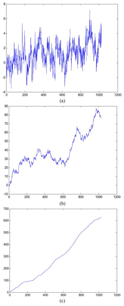
Where H is a scalar parameter 0 < H < 1 known as Hurst index (Holder exponent). The value of H determines the fBm process such that the curve B_H (t) is very rough if H = 0.01, while for H = 0.99, the curve is very smooth. Fig. 1 shows an example of simulated B_H (t) versus time plots for different H values. The figure confirms variation of surface roughness with variation of H values.

Fig. 1.

Simulation of fBm process with different H values; (a) H = 0.01; (b) H = 0.5; (c) H = 0.99.

The FD is related to the Hurst coefficient, H, as follows:

$$\text{FD}=E+1-H$$ (2)

The parameter E is Euclidean dimension (2 for 2-D, 3 for 3-D and so on) of the space.

B. Multifractal Process

Although fBm modeling has been shown useful for brain tumor texture analysis [20], considering the rough heterogeneous appearance of tumor texture in brain MRI, fBm appears homogeneous, or monofractal. In fBm process, the local degree of H is considered the same at all spatial/time variations. However, like many other real-world signals, tumor texture in MRI may exhibit multifractal structure, with H varying in space and/or time. Popescu et al. indicate that multifractal may be well suited to model processes wherein regularity varies in space as in brain MRIs [26]. Takahashi et al. [27] exploit multifractal to characterize microstructural changes of white matter in T2-weighted MRIs. Consequently, this paper proposes a model to estimate multi-FD of tumor and nontumor regions in MRI based on mBm analyses [28], [29]. In general, mBm is generalization of fBm with a zero-mean Gaussian process. The major difference between the mBm and fBm is that, contrary to fBm, the H of mBm is allowed to vary along spatial/time trajectory.

C. Classifier Boosting

Due to ineffectiveness of classifying complex tumor texture across various patients, this paper considers an ensemble boosting method. Such boosting method yields a highly accurate classifier by combining many moderately accurate component classifiers. In this method, each component classifier is successively added and trained on a subset of the training data that is “most difficult” given the current set of component classifiers already added to the ensemble. Among different variations of boosting methods, adaptive boosting such as AdaBoost [22] is the most common.

The selection of appropriate weak classifier for a specific application is an open research question. Many studies report AdaBoost with decision trees [30], neural networks [31], or support vector machine (SVM) [32] as component classifiers. Following the theoretical reasoning and experimental results reported by Li et al. [32], we consider Diverse AdaBoostSVM algorithm in our paper. The authors show that Diverse AdaBoost-SVM offers superior performance over its counterparts for unbalanced dataset. Since our brain tumor data is also unbalanced (few tumor samples compared to many nontumor samples), we believe Diverse AdaBoostSVM method is suitable for this application. The detail of Diverse AdaBoostSVM algorithm can be found in [32].

III. Mathematical Models and Algorithm

A. Multiresolution Wavelet-Based FD Estimation for Multifractal Process

In this subsection, we show formal analytical modeling of one-dimensional (1-D) multiresolution mBm to estimate the time and/or space varying scaling (or Holder) exponent H (s). We then propose an algorithm for two-dimensional (2-D) multiresolution mBm model to estimate texture feature of brain tumor tissues in MRIs.

1) One-Dimensional mBm Model and Local Scaling Exponent Estimation

The covariance function of the mBm process is defined as [33]

$${\gamma }_X(s,\tau )=\frac{{\sigma }_s^2}{2}[{\mid s\mid }^{2H(s)}+{\mid s+\tau \mid }^{2H(s)}-{\mid \tau \mid }^{2H(s)}]$$ (3)

where ${\sigma }_s^2$ is the variance of the mBm process and s, τ ∈ ℛ are two instances of time/scale. The variance of mBm increment process is given as

$$E\{{\mid x(s+\tau )-x(s)\mid }^2\}=\frac{{\sigma }_s^2}{2}{\mid \tau \mid }^{2H(s)},\tau \to 0.$$ (4)

In order to estimate Holder exponent H from multiple scales (resolutions), multiresolution wavelet is used. The wavelet transform of x (s) is denoted as

$$W_x(s,a)=\int x(\tau ){\psi }_{s,a}(\tau )d\tau$$ (5)

where ${\psi }_{s,a}(\tau )={\mid a\mid }^{-\frac{1}{2}}-\psi ({\mid a\mid }^{-1}(\tau -s))$ is the analyzing wavelet and a is the scale. The expected value of the squared-magnitude of the wavelet transform in (5) is given as

$$E\{{\mid W_x(s,a)\mid }^2\}=\iint E\{x(s)·x(s+\tau )\}{\psi }_{s,a}(\tau ){\psi }_{s+\tau ,a}(\tau )d\tau ds.$$ (6)

Substituting the autocovariance function of the mBm from (3) and ψ_s,a (τ) in (5) and choosing m = s + τ, such that dm = ds and τ − s = −m yields,

$$\begin{array}{c}E\{{\mid W_x(s,a)\mid }^2\}=a^{2H(s)+1}·\frac{{\sigma }_s^2}{2}\iint {\mid u\mid }^{2H(s)}\psi (u)\psi (v)dvdu\\ \text{for}a\to 0\text{and}0\le H(s)\le 1\end{array}$$ (7)

where ∫ ψ(u) ψ (v) dv represents the autocorrelation of the analyzing wavelet. Taking log on both sides of (7) yields

$$log(E[{\mid W_x(s,a)\mid }^2])=(2H(s)+1)\text{log}a+\text{Const.}$$ (8)

Given a single observation of the random process x, obtaining a robust estimation of the expectation of the squared magnitude of the wavelet coefficients in (8) is nontrivial. Among a few suggested techniques [34]–[36], Gonçalvès [35] obtained the empirical estimate of the qth order moment of |W_x (s, a)| as follows:

$$E\{{\mid W_x(s,a)\mid }^q\}=\frac{1}{N}\sum _{i=0}^{N-1}{\mid W_x(s_i,a)\mid }^q$$ (9)

where a single realization of the analyzed process is sampled on a uniform lattice, s_i = i/N; i = 0, …, N − 1. This estimation is based on the postulate that the wavelet series W_x (s, a) comply with the normality and stationary within scale. Substituting (9) into (8) and taking q = 2 yields,

$$2H(s)=\underset{a\to 0^{+}}{lim}\frac{log\left((1/N){\sum }_{i=0}^{N-1}{\mid W_x(s_i,a)\mid }^2\right)}{loga}.$$ (10)

For the multifractal structure, the estimated Holder regularity H (s) in (10) is neither smooth, nor continuous. To make the point-wise estimation of H(s) possible, one may relax the condition of nonsmoothness for a sufficiently small interval of time/space Δs where Δs → 0 and estimate H(s) from the observations at −(Δs/2) ≤ s ≤ s + (Δs/2). Thus, the singularity of the mBm process may be quantified around each point of time/space. The FD can be obtained using estimated H (s) in (2).

2) mBm Model and Local Scaling Exponent Estimation

In this section, a generalized 2-D method to estimate the local scaling exponent for mBm computation is proposed. Let Z (u⃗) represent a 2-D mBm process, where u⃗ denotes a position vector (u_x, u_y) of a point in the process. The properties of Z (u⃗) are similar to that of 1-D x (s) in the previous section. The 2-D correlation function of the mBm process Z (u⃗) can be defined as [37]

$$\begin{array}{l}{\gamma }_z(\overrightarrow{u},\overrightarrow{v})=E[z(\overrightarrow{u})z(\overrightarrow{v})]\\ =\frac{{\sigma }_{\stackrel{\rightharpoonup }{u}}^2}{2}[{\mid \stackrel{\rightharpoonup }{u}\mid }^{2H(\overrightarrow{u})}+{\mid \overrightarrow{v}\mid }^{2H(\overrightarrow{u})}-{\mid \overrightarrow{u}-\overrightarrow{v}\mid }^{2H(\overrightarrow{u})}]\end{array}$$ (11)

where H (ū) varies along both direction of the position vector (u_x, u_y). Let us define the continuous 2-D wavelet transform as

$$W_z(\overrightarrow{b},a)={\mid a\mid }^{-1}\int \psi ({\mid a\mid }^{-1}(\overrightarrow{u}-\overrightarrow{b}))z(\overrightarrow{u})d\overrightarrow{u}$$ (12)

where ψ(ū) is the 2-D spatial wavelet basis, a is the scaling factor, and b̄ is the 2-D translation vector.

Following (6), we obtain expected value of the magnitude square of the wavelet transform as follows:

$$E\{{\mid W_z(\overrightarrow{b},a)\mid }^2\}=\mid a^{-2}\mid \iint \psi ({\mid a\mid }^{-1}(\overrightarrow{u}-\overrightarrow{b}))\times \psi ({\mid a\mid }^{-1}(\overrightarrow{v}-\overrightarrow{b}))E\{z(\overrightarrow{u})z(\overrightarrow{v})\}d\overrightarrow{u}d\overrightarrow{v}.$$ (13)

Substituting (11) into (12), and changing the variables of integration to p̄ = (ū − v̄)/a and q̄ = (v̄ − b̄/a yields

$$E\{{\mid W_z(\overrightarrow{b},a)\mid }^2\}=a^{2H(\overrightarrow{u})+2}\frac{{\sigma }_s^2}{2}\iint {\mid \overrightarrow{u}\mid }^{2H(\overrightarrow{u})}\times \psi (\stackrel{\rightharpoonup }{u})\psi (\overrightarrow{v})d\overrightarrow{v}d\overrightarrow{u},\text{for}a\to 0.$$ (14)

Taking the logarithm on both sides of (14) yields

$$log(E[{\mid W_z(\overrightarrow{b},a)\mid }^2])=(2H(\stackrel{\rightharpoonup }{u})+2)loga+\text{Const.}$$ (15)

Following the steps similar to previous section one can estimate the E{|W_z (b⃗, a)|²} as follows:

$$E\{{\mid W_z(\stackrel{\rightharpoonup }{b},a)\mid }^2\}=\frac{1}{M+N}\sum _{x=0}^{N-1}\sum _{y=0}^{M-1}{\mid W_z(b_{x,y},a)\mid }^2$$ (16)

where a single realization of the analyzed 2-D process is sampled on a uniform 2-D lattice b_x,y = [(x/N, y/M); x = 0, …, N − 1, y = 0, …, M − 1]. Thus, one may approximate H (u⃗) for a 2-D mBm process as follows:

$$2H(\stackrel{\rightharpoonup }{u})=\underset{a\to 0^{+}}{lim}\frac{log\left((1/(M+N)){\sum }_{x=0}^{N-1}{\sum }_{y=0}^{M-1}{\mid W_z(b_{x,y},a)\mid }^2\right)}{loga}.$$ (17)

Following the same arguments for 1-D mBm in the previous section, one may estimate H(u⃗) from the observations of sufficiently small area Δu⃗ (Δu_x, Δu_y) around u⃗ where Δu_x → 0 and Δu_y → 0. The above derivation can be generalized to estimate mBm in 3-D or higher dimension.

B. Algorithms for Texture Modeling Using mBm

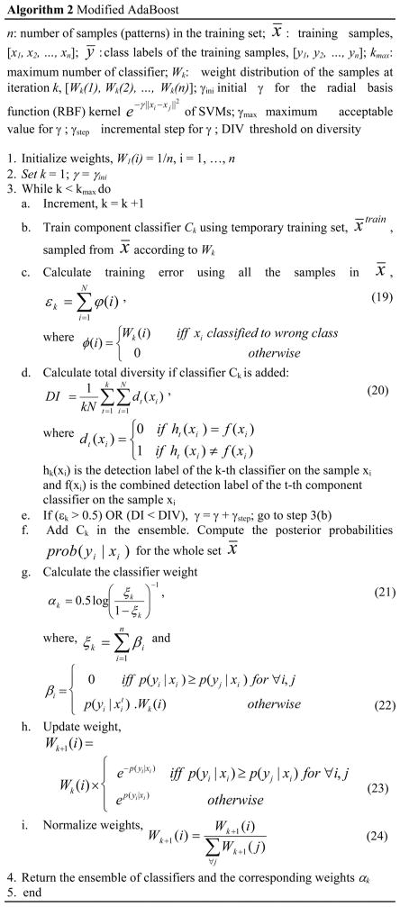
Fig. 2 shows a formal algorithm to estimate the multi-FD. We first divide the image into nonoverlapping blocks or subimages. The second moment of selected type of wavelet for every subimage is computed in multiple different scales as shown in (16). Then, the holder exponent is computed from the linear regression of moments versus the scale in a log-log plot as shown in (17). Finally, FD is computed using (2).

Fig. 2.

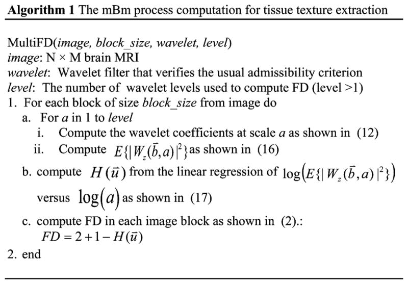
Algorithm to compute multi-FD in brain MRI.

C. Algorithm for AdaBoost Enhancement

This section discusses novel extensions of the DiverseAdaBoostSVM to improve tumor classification rate. The resulting enhanced AdaBoost algorithm is shown in Fig. 3. Fig. 3 briefly summarizes our changes to original Diverse AdaboostSVM method [32]. The first modification is in step 3(g) where the weights of the component classifiers are obtained. These weights are inversely proportional to three factors such as: 1) how many samples are misclassified; 2) how confidently the samples are misclassified; and 3) how difficult the misclassified samples are. Both “confidence” and “difficultness” are closely related. Here is the shuttle difference: “difficultness” of samples is represented by the weights W_k (i) that carry over the classification results from previous iterations. So, if one sample is misclassified many times in different iterations, the weight of that sample is likely to be high compared with the one that has been misclassified in only few times in previous iterations. On the other hand, “confidence” is measured based on current iteration only. We represent confidence using the probability p(y_i |x_i). If one sample is misclassified with high probability, we penalize the corresponding classifier k more compared with the classifier that misclassifies the same sample with low probability.

Fig. 3.

Proposed modified AdaBoost algorithm.

The standard AdaBoost algorithm, in contrast with ours, does not consider the confidence in computing the classifier weights. The next improvement is shown in step 3(h). The weights (probability of being selected in the next cycle) are updated for each training sample considering how confidently that specific sample is classified (or misclassified) in the current cycle. Standard AdaBoost algorithm changes weights of each sample equally based on the classification error of the last component classifier. Note that in standard AdaBoost, the classification error is computed based on the crisp classification decision that does not account for the confidence/probability of such decision.

The detection decision on a new sample x can be based on the weighted vote of the component classifiers

$$D(x)=\sum _{\forall k}{\alpha }_k{d}_k(x)$$ (18)

where d (x) is class decision from each component classifiers and D (x) is the final decision.

Note if SVM is added to the AdaBoost in an unconstrained manner, the performance may degrade since each additional SVM may be actually a “weak learner” [38]. However, in our framework, we never add any new SVM unless the total diversity, as defined in (20), goes up. That is how the overall classification performance is expected to increase. Fig. 11 shows that the classification error decreases as we add more and more component (weak) learner.

Fig. 11.

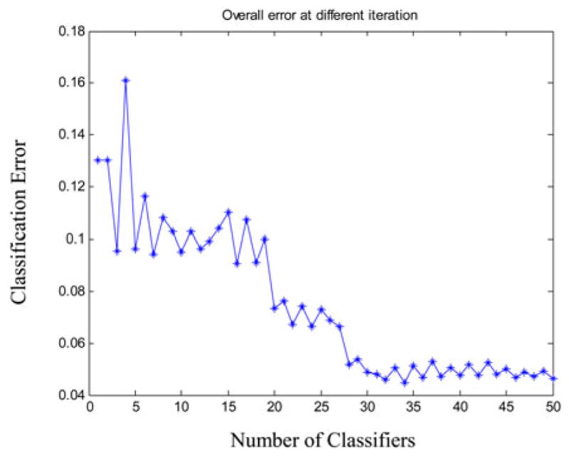
Change in classification error as classifiers are added in the ensemble.

Our choice of SVM classifier as “weak learner” (e.g., “component classifier”) is inspired by the interesting work of Li et al. [32]. Li et al. showed how the choice of SVM outperforms the other choices. In addition, they claim that their framework is not affected by unbalanced dataset like ours (number of tumor samples is way less than the number of nontumor samples). Finally, our proposed AdaBoost framework is not dependent on any specific choice of “weak learner”.

IV. Data

The brain tumor MRI data in this study consists of 3 different modalities, such as T1-weighted (nonenhanced), T2-weighted, and FLAIR from 14 different pediatric patients with total of 309 tumor bearing image slices. Patients consist of two different tumor groups such as 6 patients (99 MRI slices) are from astrocytoma and 8 patients (210 MRI slices) are from medulloblastoma tumor types, respectively. All the slices are obtained from Axial perspective.

All of these MRIs are sampled by 1.5 T Siemens Magnetom scanners from Siemens Medical Systems. The slice thickness is 8–10 mm, with the slice gap of 1–12 mm, the field-of-view (FOV) is 280–300 × 280–300 mm², the image matrix is of (256 × 256) or (512 × 512) pixels and 16 bits/pixel.

V. Fractal-Based Tumor Detection and Classification

In this study, we fuse the existing PTPSA fractal and newly proposed multi-FD features in automatic tumor segmentation in brain MRI. In addition, we extract texton feature [15] for comparison in segmenting brain tumors. The overall flow diagram is shown in Fig. 4. Following standard preprocessing steps for brain MRI, we extract corresponding fractal, texton, and intensity features for all 14 patients in this study. In the next step, different combinations of feature sets are exploited for tumor segmentation and classification. Feature values are then directly fed to the AdaBoost classifier for classification of tumor and nontumor regions. Manual labeling to tumor regions is performed for supervised classifier training. The trained classifiers are then used to detect the tumor or nontumor segments in unknown brain MRI. In the following subsections, we describe these steps in more details.

Fig. 4.

Simplified overall flow diagram.

A. MRI Preprocessing

The proposed methods in this paper involve feature fusion from different MRI modalities. Therefore, different MRI volumes need to be aligned. The following preprocessing steps are performed on the MRI volumes:

1. Realign and unwarp slices within a volume, separately for every modality and every patient using SPM8 toolbox.

2. Co-register slices from different modalities with the corresponding slices of T1-weighted (nonenhanced) slices using SPM8 toolbox for each patient.

The PTPSA, texton, and multi-FD texture features are extracted after the above mentioned preprocessing steps. In addition, for intensity features, the following two preprocessing steps are also performed on all MRI modalities (T1, T2, FLAIR) available in our dataset:

1. Correct MRI bias field using SPM8 toolbox.

2. Correct bias and intensity inhomogeneity across all the slices of all the patients for each MRI modality using two-step normalization method [39]. Note that we extract the fractal features before bias field and intensity inhomogeneity correction. As described in [40], the multiscale wavelets do not require these corrections.

Finally, BET toolbox is used to extract brain tissue from skull. Fig. 5 illustrates an example of different preprocessing steps in multimodality brain tumor MRI patients in our dataset.

Fig. 5.

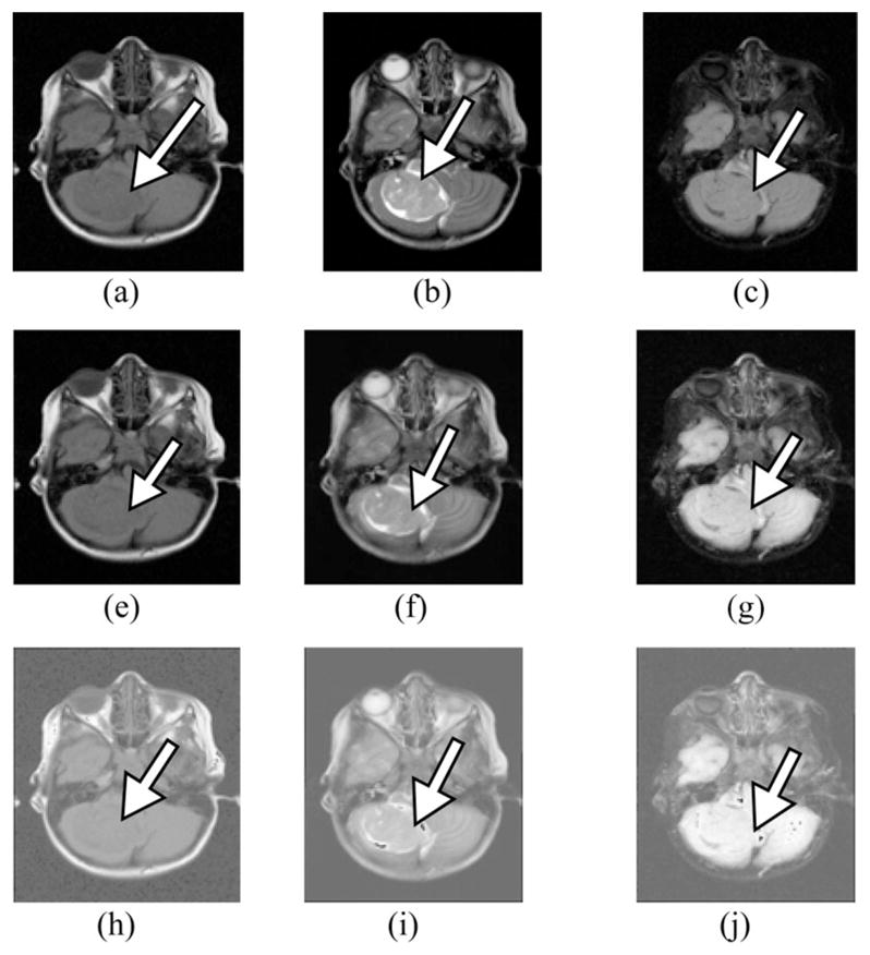
Multimodality MRI slices showing different preprocessing steps: (a) original T1, (b) original T2, (c) original FLAIR, (e) T1 after realign, unwarp, and bias field correction, (f) T2 after realign, unwarp, co-registration with T1 and biasfield correction, (g) FLAIR after realign, unwarp, co-registration with T1 and bias field correction, (h) intensity normalized T1, (i) intensity normalized T2, and (j) intensity normalized FLAIR.

B. Feature Set

As discussed in Section II-A, the feature set includes intensity, texton [16], PTPSA [1], and multi-FD (shown in Fig. 2). We represent 3-D segmentation process into a sequence of 2-D segmentations (at pixel level) since the prevailing practice of the radiologists in the radiology reading room is to analyze sequence of 2-D MRI slices side-by-side for tumor detection and segmentation. However, there is no theoretical limitation to extend this computation to 3-D. Each pixel of a slice is represented by a set of feature values. Each of intensity, PTPSA and multi-FD is represented by single feature values, while texton is represented by a vector of 48 feature values (corresponding to 48 filters [15]). For both multi-FD and PTPSA, we first divide the image into nonoverlapping subimages. In our experiment, we obtain the best result for subimage size of 8 × 8. Furthermore, as suggested by the mathematical derivation in previous section, multiresolution computation employing first two scales with a wavelet such as Daubechies is used for this paper.

C. Brain Tumor Segmentation and Classification from Nontumor Tissue

For tumor/nontumor tissue segmentation and classification, MRI pixels are considered as samples. These samples are represented by a set of feature values extracted from different MRI modalities. Features from all modalities are fused for tumor segmentation and classification. We follow data driven machine learning approach to fuse different features extracted from different MRI modalities. We let our supervised classifier autonomously exploit multiple features extracted from different modalities in the training dataset. Different feature combinations (as described in Section VI), are used for comparison. A modified supervised AdaBoost ensemble of classifier is trained to differentiate tumor from the nontumor tissues. Since the features are extracted in 2-D, each sample represents a pixel instead of a voxel. However, the proposed classification framework can readily be extended to 3-D segmentation without any modification. For supervised training purpose, manually labeled ground truths of tumor core and nontumor regions are used. For our dataset, ground truth labels are obtained from combination of T1, T2, and FLAIR modalities by the radiologists.

D. Performance Evaluation

Receiver operating characteristic (ROC) curves are obtained to ascertain the sensitivity and specificity of the classifiers. In this study, we define TPF as the proportion of the tumor pixels that are correctly classified as tumor by the classifier while we define FPF as the proportion of the nontumor pixels that are incorrectly classified as tumor by the classifier. In addition, few similarity coefficients are used to evaluate the performance of tumor segmentation. The similarity coefficients used in this study include: Jaccard [a/(a + b)], Dice [2a/(2a + b)], Sokal and Sneath [a/(a + 2b)], and Roger and Tanimoto [(a + c)/(a + 2b + c)] coefficients, where a is the number of samples where both the classifier decision and the manual label confirms the presence of tumor; b is the number of samples where the decisions mismatch; and c is the number of samples where both the classifier decision and the manual label confirms the absence of tumor.

VI. Experimental Results and Discussions

This section reports results and analyses. Fig. 6 shows an example MRI slice and corresponding scatter plots comparing feature values between tumor and nontumor regions. The points in scatter plots represent average feature values within an 8 × 8 subimage in an MRI for a patient. The black points represent average feature values in tumor regions, while the white points represent the same in nontumor regions. Fig. 6(b)–(d) shows the plots of PTPSA (fractal) versus intensity, multi-FD versus intensity and multi-FD versus PTPSA versus intensity features, respectively. These plots suggest that features representing tumor regions are well separated from that of the non-tumor regions.

Fig. 6.

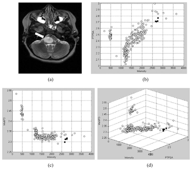
(a) Original T2 MRI. Arrow shows the tumor location. Features plots for (b) FD (PTPSA) versus intensity; (c) multi-FD versus intensity; (d) multi-FD versus intensity versus FD (PTPSA). Black points represent feature values in tumor regions, while white points represent feature values in nontumor regions.

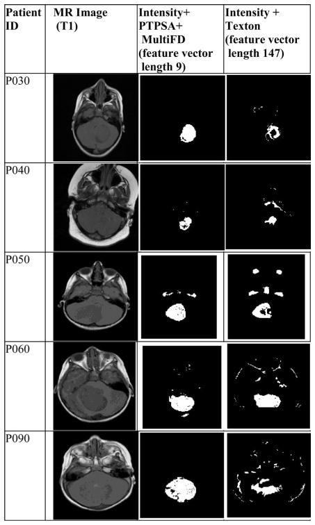
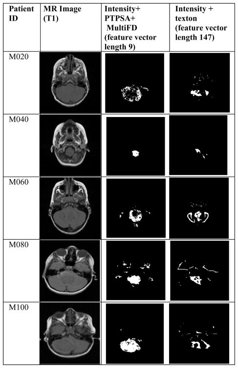
Figs. 7 and 8 show examples of tumor segmentation results for four astrocytoma and medulloblastoma patients, respectively. The slices are randomly chosen from corresponding patient MRI volumes. The figures compare tumor segmentation results between (intensity, PTPSA, and multi-FD) and (intensity and texton) feature combinations. Notice (intensity, PTPSA, and multi-FD) feature combination captures more tumor regions for three astrocytoma (P030, P040, and P090) and three medulloblastoma (M020, M040, and M100) patients, respectively. Furthermore, the same feature combination also shows superiority in correctly classifying nontumor regions for two astrocytoma (P040 and P060) and three medulloblastoma (P090, M040, and M060) patients, respectively. Therefore, it is clear from visual observation that (intensity, PTPSA and multi-FD) feature combination offers better tumor segmentation. Quantitative analyses with the whole dataset is shown later in this section.

Fig. 7.

Comparison of segmentation results using (intensity, PTPSA and multi-FD) versus (intensity and texton) feature combination for astrocytoma (PXXX) patients.

Fig. 8.

Comparison of segmentation results using (intensity, PTPSA and multi-FD) versus (intensity and texton) feature combination for medulloblastoma (MXXX) patients.

Since our dataset does not have enough sagittal or coronal slices from all different modalities, most of the results presented here are based on axial slices only. However, for completeness, we report two segmentation results using intensity, PTPSA and multi-FD in Figs. 9 and 10. Fig. 9 uses sagittal slice from T1 and T1 contrast enhanced, while Fig. 10 uses coronal slices from T2 and T1 contrast modalities (no other modalities are available), respectively.

Fig. 9.

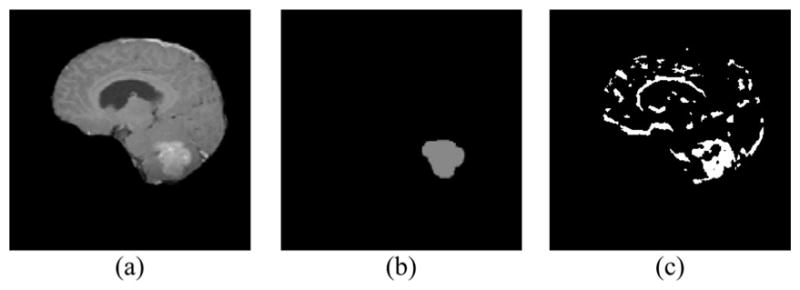
Sagittal slice: (a) T1 contrast enhanced; (b) ground Truth; (c) Segmented tumor cluster.

Fig. 10.

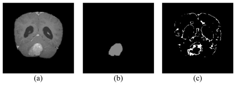
Coronal slice: (a) T1 contrast enhanced; (b) ground truth; (c) segmented tumor cluster.

The performance of the proposed modified AdaBoost algorithm is characterized next. Fig. 11 shows how the overall classification error on trained data changes as more classifiers are added. As expected, the overall error initially decreases as more component classifier is added. Similarly, Fig. 12 shows how the total diversity of the ensemble of classifier changes as classifiers are added. We observe that at some points total diversity does not improve further with inclusion of more classifiers. In boosting, having diversity among classifiers is considered an important factor. Therefore, Fig. 12 suggests that for our dataset, using 10–20 classifiers may be sufficient.

Fig. 12.

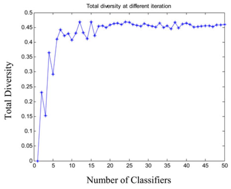
Change in total diversity as classifiers are added in the ensemble.

Fig. 13 shows ROC curve using average performance measure values for six astrocytoma patients (99 MRI slices; 256 × 256 or 512 × 512 pixels in each slice). We use different feature combinations such as (a) intensity and PTPSA, (b) intensity and multi-FD, (c) intensity, PTPSA, and multi-FD, (d) intensity and texton, and (e) intensity, PTPSA, multi-FD, and texton. TPF and FPF values are obtained at different decision thresholds between [−1,1]. Comparison among the ROCs obtained from intensity, PTPSA and multi-FD combination and those obtained from texton combination show that one can achieve better TPF (Y -axis) sacrificing much less FPF (X-axis) in tumor segmentation. We observe similar performance with eight medulloblastoma patients as well (not shown due to space limitation). Fig. 14 shows how the classifier prediction values vary when they are trained with different feature combinations specified above. Each column is a box and whisker plot of prediction values that corresponds to either tumor or nontumor samples. In x-axis, the letters before hyphen correspond to one of the feature combinations (such as IP), while the digit after hyphen specifies if the box plot corresponds to tumor (1) or nontumor (0) samples. In each box plot, box is drawn between lower and upper quartile of prediction values and includes a splitting line at the median. The whiskers are extended from the box end to 1.5 times the box length. Outliers (values beyond the whiskers) are displayed with a “+” sign. Comparison of box plot median values is similar to visual hypothesis test, or analogous to the t-test used for comparison of mean values. The box length and whisker positions can be representative of the dispersion of prediction values. Note for intensity and multi-FD (IM) feature combination, the dispersion of prediction values is very low for both tumor and nontumor samples. This is not true for any other feature combinations.

Fig. 13.

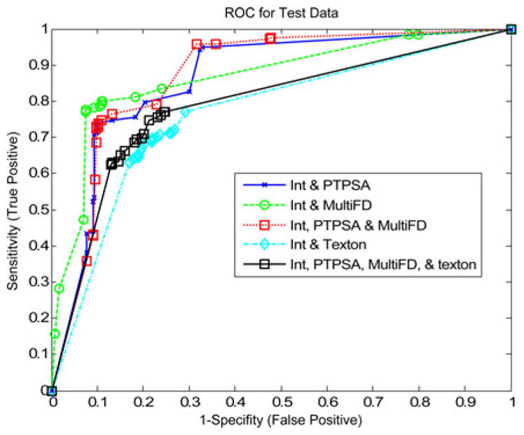
ROC curve obtained from astrocytoma patients with: (a) intensity and PTPSA, (b) intensity and multi-FD, (c) intensity, PTPSA, and multi-FD, (d) intensity and texton, and (e) intensity, PTPSA, multi-FD, and texton.

Fig. 14.

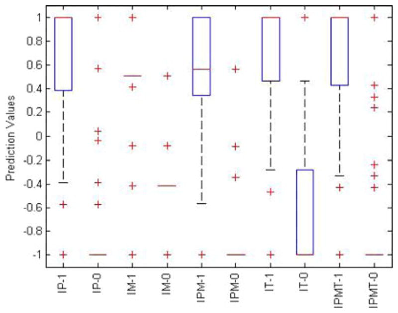
Box plot of modified AdaBoost prediction values for tumor (1) and nontumor (0) samples. Classifiers are trained with different feature combinations (IP: intensity+PTPSA, IM: intensity+multi-FD, IPM: intensity+PTPSA+multi-FD, IT: intensity+texton, IPMT: intensity+ PTPSA+multi-FD+texton).

We demonstrate more quantitative performance comparison between our proposed modified AdaBoost with the AdaBoost algorithm [32] without modification. Table I shows classifier performance and overlap metrics for eight medulloblastoma patients. For this experiment, feature vector is composed of intensity, PTPSA, and multi-FD from T1, T2, and FLAIR modalities. In rows 1 and 2 of Table I, measures obtained at a fixed decision threshold 0 are shown. The modified AdaBoost achieves better TPF compared to that of the original AdaBoost in [32]. Similar performance improvement is also observed using our modified AdaBoost algorithm for the astrocytoma patients (not shown due to space limitation).

TABLE I.

Metrics Comparing the Classifier Performances for Eight Medulloblastoma Patients

Classifier	TPF	FPF	Jaccard	Dice	Sokal & Sneath	Roger & Tanimoto
AdaBoost [33] at thresh=0	0.79	0.36	0.58	0.73	0.41	0.55
Proposed AdaBoost at thresh=0	0.81	0.39	0.58	0.73	0.41	0.55

Finally, for quantitative segmentation performance comparison using different feature combinations, we fix decision threshold at “0” and obtain classifier performance and overlap metrics values. The values are summarized in Table II for six astrocytoma patients (99 MRI slices; 256 × 256 or 512 × 512 pixels in each slice). The highest performing metrics are denoted in bold face in each column. Note that the Intensity and multi-FD feature combination offers the best TPF and similarity overlap values when compared to all other combinations in Table II. Similar performance improvements using multi-FD feature for medulloblastoma patients are also observed (not shown due to space limitation). In summary, it is worth noting that intensity and fractal feature combinations outperform Gabor-like features for brain tumor segmentation performance. Also note that combining intensity and fractal with Gabor-like texton features may not improve the brain tumor segmentation performance for these patients in this study.

TABLE II.

Performance Measure at Decision Threshold “0” for Six Astrocytoma Patients

Feature	TPF	FPF	Jaccard	Dice	Sokal & Sneath	Roger & Tanimoto
Intensity+ PTPSA	0.73	0.10	0.65	0.79	0.49	0.68
Intensity+ MultiFD	0.79	0.11	0.71	0.83	0.55	0.73
Intensity+ PTPSA+ MultiFD	0.74	0.10	0.65	0.79	0.49	0.68
Intensity+ Texton	0.69	0.22	0.55	0.71	0.38	0.57
Intensity+ PTPSA+ MultiFD+ Texton	0.70	0.19	0.57	0.73	0.40	0.59

In order to compare performance with other state-of-the-art work, we applied our proposed tumor segmentation technique on publicly available MICCAI BRATS2012 dataset [42]. We select ten low-grade glioma patients with 1492 tumor slices in four different modalities. We select low-grade glioma patients since such cases may pose increased difficulty in segmentation compared to high grade. Note we use T1 contrast enhanced, T1, T2, and FLAIR MRI for the pre-processing steps as discussed in Section V-A for this BRATS2012 dataset.

We predict the binary classification of tumor core versus rest (tumor plus nontumor region) labels. Note we do not predict edema label since the goal of this paper is only tumor segmentation. All the subsequent results are obtained by using the BRATS online evaluation tool [42]. Table III shows the summary of results for this dataset. In BRATS2012 ground truth notation, active core tumor is labeled as 2 and the nontumor (the rest) as 0. We follow these notations for our evaluations in this paper. The second column in Table III shows segmentation results for our technique. These results are obtained using intensity and multi-FD features from T1, T1 contrast enhanced, T2, and FLAIR modalities. Notice the intensity and multi-FD feature combination is used following improved performance results as shown in Fig. 13 and Table II, respectively. For within patient segmentation using 10 low-grade cases, we use fivefold cross validation. Table III shows that our segmentation results (dice overlap) is more consistent and on the average outperforms the other methods for this dataset. Table IV shows the segmentation result on BRATS challenge/testing dataset of four low-grade patients (across patient results). Here, the training is done with the BRATS training dataset. The average mean dice score (0.33) is among the few top performing works that have been published reporting BRTAS2012 competition results. To understand the generalization trends between our dataset (as described in Section IV) and the BRATS dataset, we train the model with our astrocytoma (low-grade) dataset, and test on both BRATS low-grade training and test data. The results are shown in Tables V and VI for BRATS training and test dataset, respectively. The mean results from both cases show moderate to low performance due to the heterogeneity of tumor type, appearance, imaging modalities, center and imaging device specific variability. All results in this paper are obtained using MATLAB 2011 a on windows 64 bit 2.26 GHz Intel(R) Xeon(R) processor, with 4 GHz RAM. The training time varies from 2 to 4 days per patient. Prediction time varies from 1.5 to 2 min per slice.

TABLE III.

Performance Comparison on Brats 2012 Training Data With Other Works (Dice Overlap)

Patient ID	Our Method	[43]	[17]	[16]*	[18]	[41]	[19]
L001	0.83	0.78	0.83	--	0.83	0.84	0.84
L002	0.65	0.68	0.32	--	0.55	0.11	0.24
L004	0.52	0.02	0.05	--	0.61	0.01	0.02
L006	0.62	0.35	0.18	--	0.71	0.59	0.73
L008	0.80	0.84	0.44	--	0.78	0.68	0.00
L011	0.90	0.86	0.14	--	0.88	0.00	0.00
L012	0.78	0.74	0.00	--	0.81	0.01	0.82
L013	0.64	0.30	0.00	--	0.48	0.17	0.45
L014	0.78	0.84	0.00	--	0.73	0.00	0.00
L015	0.78	0.75	0.00	--	0.75	0.00	0.12
mean	0.73	0.62	0.20	0.49±0.26	0.71	0.24	0.32

^*The missing data are not reported in [16].

TABLE IV.

Performance Comparison on Brats-2012 Challenge Data With Other Works (Dice Overlap)

Patient ID	Our Method	[43]*	[16]*	[18]*
L103	0.463	--	--	--
L105	0.052	--	--	--
L109	0.803	--	--	--
L116	0.003	--	--	--
Mean	0.330	0.339	0.332	0.324

^*The missing data are not reported in [43], [16], [18].

TABLE V.

Dataset Cross-Validation Performance on Brats-2012 Training Data (Dice Overlap); Model Trained on Our Astrocytoma^* Data

Patient ID	L001	L002	L004	L006	L008	Overall Mean
Dice	0.556	0.470	0.340	0.274	0.546	0.484
Patient ID	L011	L012	L13	L014	L015
Dice	0.818	0.666	0.184	0.429	0.552

^*Our Astrocytoma data contains the low-grade tumor.

TABLE VI.

Dataset Cross-Validation Performance on Brats-2012 Test Data (Dice Overlap); Model Trained on Our Astrocytoma Data

Patient ID	L103	L105	L109	L116	Overall Mean
Dice	0.213	0.023	0.695	0	0.233

VII. Conclusion and Future Works

In this paper, novel multifractal (multi-FD) feature extraction and supervised classification techniques for improved brain tumor detection and segmentation are proposed. The multi-FD feature characterizes intricate tumor tissue texture in brain MRI as a spatially varying multifractal process in brain MRI. On the other hand, the proposed modified AdaBoost algorithm considers wide variability in texture features across hundreds of multiple-patient MRI slices for improved tumor and nontumor tissue classification. Experimental results with 14 patients involving 309 MRI slices confirm the efficacy of novel multi-FD feature and modified AdaBoost classifier for automatic patient independent tumor segmentation. In addition, comparison with other state-of-the-art brain tumor segmentation techniques with publicly available low-grade glioma in BRATS2012 dataset shows that our methods outperform other methods for most of these patients. Note our proposed feature-based brain tumor segmentation does not require deformable image registration with any predefined atlas. The computation complexity of multi-FD feature is liner and increases with slice resolution (number of pixel), block size, and the number of wavelet levels. Likewise the computation complexity for our modified AdaBoost algorithm is linear and increases with number of samples times number of component classifiers. As a future direction, incorporating information from registered atlas may prove useful for segmentation of more subtle and complex tumors. In addition, it may be interesting to investigate the proposed modified AdaBoost classification method when one incorporates atlas based prior information in the segmentation framework.

Biographies

Atiq Islam received the B.Sc. degree in electronics and computer science from Jahangirnagar University (JU), Savar, Bangladesh, in 1998, the M.S. degree in computer science from Wright State University, Dayton, OH, USA, in 2002, and the Ph.D. degree in computer engineering from the University of Memphis, Memphis, TN, USA, in 2008.

He is currently a Senior Applied Researcher at eBay Inc., San Jose, CA, USA. He was an Applied Researcher with a number of research team in Silicon Valley, CA, USA (Sony, Google, Ooyala, and Sportvision). He was a Lecturer at JU from 1999 to 2001. His current research interests include machine learning, image processing, and computer vision where he enjoys discovering interesting patterns from image, text, video or speech. He has authored or coauthored more than a dozen refereed journal papers, book chapters, patents and conferences proceedings.

Syed M. S. Reza received the B.Sc. degree in electrical and electronics engineering from Bangladesh University of Engineering and Technology, Dhaka, Bangladesh, in 2007. He is currently working toward the Ph.D. degree in electrical and computer engineering at Old Dominion University, Norfolk, VA, USA.

His current research interest includes image processing focusing on medical images, automatic segmentation of brain tumors in MR Images.

Khan M. Iftekharuddin (SM’02) received the B.Sc. degree in electrical and electronic engineering from Bangladesh Institute of Technology, Bangladesh, in 1989, and the M.S. and Ph.D. degrees in electrical and computer engineering from the University of Dayton, OH, USA, in 1991 and 1995 respectively.

He is currently a Professor in the Department of Electrical and Computer Engineering at Old Dominion University (ODU), Norfolk, VA, USA, where he is the Director of ODU Vision Lab and a Member of Biomedical Engineering Program. His current research interests include computational modeling of intelligent systems and reinforcement learning, stochastic medical image analysis, intersection of bioinformatics and medical image analysis, distortion-invariant automatic target recognition, biologically inspired human and machine centric recognition, recurrent networks for vision processing, machine learning for robotics, emotion detection from speech and discourse, and sensor signal acquisition and modeling. Different federal, private funding agencies and industries such as NSF, NIH, NASA, ARO, AFOSR, NAVY, DOT, the Whitaker Foundation, St. Jude Children’s Research Hospital, Southern College of Optometry (Assisi Foundation), Upper Great Plain Transportation Institute, FedEx, and Timken Research have funded his research. He is the author of one book, several book chapters, and over 150 refereed journal and conference papers. He is an Associate Editor for a number of journals including Optical Engineering.

Dr. Iftekharuddin is a Fellow of SPIE, a Senior Member of the IEEE CIS, and a member of the Optical Society of America (OSA).

References

- 1.Iftekharuddin KM, Jia W, March R. Fractal analysis of tumor in brain MR images. Mach Vision Appl. 2003;13:352–362. [Google Scholar]
- 2.Lee CH, Schmidt M, Murtha A, Bistritz A, Sander J, Greiner R. Segmenting brain tumor with conditional random fields and support vector machines. Proc Int Conf Comput Vision. 2005:469–478. [Google Scholar]
- 3.Corso JJ, Yuille AL, Sicotte NL, Toga AW. Detection and segmentation of pathological structures by the extended graph-shifts algorithm. Med Image Comput Comput Aided Intervention. 2007;1:985–994. doi: 10.1007/978-3-540-75757-3_119. [DOI] [PubMed] [Google Scholar]
- 4.Cobzas D, Birkbeck N, Schmidt M, Jagersand M, Murtha A. 3-D variational brain tumor segmentation using a high dimensional feature set. Proc IEEE 11th Int Conf Comput Vision. 2007:1–8. [Google Scholar]
- 5.Wels M, Carneiro G, Aplas A, Huber M, Hornegger J, Comaniciu D. A discriminative model-constrained graph cuts approach to fully automated pediatric brain tumor segmentation in 3-D MRI. Lecture Notes Comput Sci. 2008;5241:67–75. doi: 10.1007/978-3-540-85988-8_9. [DOI] [PubMed] [Google Scholar]
- 6.Lopes R, Dubois P, Bhouri I, Bedoui MH, Maouche S, Betrouni N. Local fractal and multifractal features for volumic texture characterization. Pattern Recog. 2011;44(8):1690–1697. [Google Scholar]
- 7.Islam A, Iftekharuddin K, Ogg R, Laningham F, Sivakumar B. Multifractal modeling, segmentation, prediction and statistical validation of posterior fossa tumors. Proc SPIE Med Imaging: Comput-Aided Diagnosis. 2008;6915:69153C-1–69153C-2. [Google Scholar]
- 8.Wang T, Cheng I, Basu A. Fluid vector flow and applications in brain tumor segmentation. IEEE Trans Biomed Eng. 2009 Mar;56(3):781–789. doi: 10.1109/TBME.2009.2012423. [DOI] [PubMed] [Google Scholar]
- 9.Prastawa M, Bullitt E, Moon N, Van Leemput K, Gerig G. Automatic brain tumor segmentation by subject specific modification of atlas priors. Acad Radiol. 2003;10:1341–1348. doi: 10.1016/s1076-6332(03)00506-3. [DOI] [PMC free article] [PubMed] [Google Scholar]
- 10.Warfield S, Kaus M, Jolesz F, Kikinis R. Adaptive template moderated spatially varying statistical classification. Med Image Anal. 2000 Mar;4(1):43–55. doi: 10.1016/s1361-8415(00)00003-7. [DOI] [PubMed] [Google Scholar]
- 11.Kaus MR, Warfield SK, Nabavi A, Black PM, Jolesz FA, Kikinis R. Automated segmentation of MR images of brain tumors. Radiology. 2001;218(2):586–91. doi: 10.1148/radiology.218.2.r01fe44586. [DOI] [PubMed] [Google Scholar]
- 12.Gering D, Grimson W, Kikinis R. Recognizing deviations from normalcy for brain tumor segmentation. Proc Int Conf Med Image Comput Assist Interv. 2005;5:508–515. [Google Scholar]
- 13.Davatzikos C, Shen D, Mohamed A, Kyriacou S. A framework for predictive modeling of anatomical deformations. IEEE Trans Med Imaging. 2001 Aug;20(8):836–843. doi: 10.1109/42.938251. [DOI] [PubMed] [Google Scholar]
- 14.Menze BH, Leemput KV, Lashkari D, Weber MA, Ayache N, Golland P. A generative model for brain tumor segmentation in multimodal images. In: Navab N, Pluim JPW, Viergever MA, Jiang T, editors. Medical Image Computing and Computer-Assisted Intervention—MICCAI 2010. Berlin, Germany: Springer; 2010. pp. 151–159. [DOI] [PMC free article] [PubMed] [Google Scholar]
- 15.Leung T, Malik J. Representing and recognizing the visual appearance of materials using three-dimensional textons. Int J Comput Vision. 2001;43(1):29–44. [Google Scholar]
- 16.Bauer S, Fejes T, Slotboom J, Weist R, Nolte LP, Reyes M. Segmentation of brain tumor images based on integrated hierarchical classification and regularization. Proc MICCAI-BRATS. 2012:10–13. [Google Scholar]
- 17.Geremia E, Menze BH, Ayache N. Spatial decision forest for glioma segmentation in multi-channel MR images. Proc MICCAI-BRATS. 2012:14–18. doi: 10.1007/978-3-642-15705-9_14. [DOI] [PubMed] [Google Scholar]
- 18.Hamamci A, Unal G. Multimodal brain tumor segmentation using the tumor-cut method on the BraTS dataset. Proc MICCAI-BRATS. 2012:19–23. [Google Scholar]
- 19.Raviv TR, Leemput KV, Menze BH. Multi-modal brain tumor segmentation via latent atlases. Proc MICCAI-BRATS. 2012:64–73. [Google Scholar]
- 20.Iftekharuddin KM, Islam A, Shaik J, Parra C, Ogg R. Automatic brain tumor detection in MRI: methodology and statistical validation. Proc SPIE Symp Med Imaging. 2005;5747:2012–2022. [Google Scholar]
- 21.Ahmed S, Iftekharuddin K, Vossough A. Efficacy of texture, shape, and intensity feature fusion for posterior-fossa tumor segmentation in MRI. IEEE Trans Inf Technol Biomed. 2011 Mar;15(2):206–213. doi: 10.1109/TITB.2011.2104376. [DOI] [PubMed] [Google Scholar]
- 22.Freund Y, Schapire RE. A decision-theoretic generalization of online learning and an application to boosting. Comput Syst Sci. 1997;55(1):119–139. [Google Scholar]
- 23.Pentland AP. Fractal-based description of natural scenes. IEEE Trans Pattern Anal Mach Intell. 1984 Nov;6(6):661–674. doi: 10.1109/tpami.1984.4767591. [DOI] [PubMed] [Google Scholar]
- 24.Zook JM, Iftekharuddin KM. Statistical analysis of fractal-based brain tumor detection algorithms. Magn Resonance Imag. 2005;23(5):671–678. doi: 10.1016/j.mri.2005.04.002. [DOI] [PubMed] [Google Scholar]
- 25.Flandrin P. Wavelet analysis and synthesis of fractional Brownian motion. IEEE Trans Info Theory. 1992 Mar;38(2):910–917. [Google Scholar]
- 26.Popescu BP, Vehel JL. Stochastic fractal models for image processing. IEEE Signal Proc Mag. 2002 Sep;19(5):48–62. [Google Scholar]
- 27.Takahashi K, Murata T, Narita K, Hamada T, Kosaka H, Omori M, Kimura H, Yoshida H, Wada Y, Takahashi T. Multifractal analysis of deep white matter microstructural changes on MRI in relation to early-stage atherosclerosis. Neuroimage. 2006;32(3):1158–66. doi: 10.1016/j.neuroimage.2006.04.218. [DOI] [PubMed] [Google Scholar]
- 28.Peltier RF, Vehel JL. Multifractional Brownian motion: Definition and preliminary results. INRIA. 1995 Project 2645.
- 29.Flandrin P, Gonçalvès P. Scaling exponents estimation from time-scale energy distributions. Proc IEEE Int Conf Acoust, Speech Signal. 1992:V.157–V.160. [Google Scholar]
- 30.Dietterich TG. An experimental comparison of three methods for constructing ensembles of decision trees: Bagging, boosting, and randomization. Mach Learning. 2000;40(2):139–157. [Google Scholar]
- 31.Ratsch G, Onoda T, Muller KR. Soft margins for adaboost. Mach Learning. 2001;42(3):287–320. [Google Scholar]
- 32.Li X, Wang L, Sung E. AdaBoost with SVM based component classifier. Eng Appl Artif Intell. 2008;21(5):785–795. [Google Scholar]
- 33.Gonçalvès P, Abry P. Multiple-window wavelet transform and local scaling exponent estimation. Proc IEEE Int Conf Acoustics, Speech Signal Proc. 1997;5:3433–3436. [Google Scholar]
- 34.Gonçalvès P, Riedi R, Baraniuk R. A simple statistical analysis of wavelet-based multifractal spectrum estimation. Proc Asilomar Conf Signals, Syst Comput. 1998;1:287–291. [Google Scholar]
- 35.Gonçalvès P. Existence test of moments: Application to multifractal analysis. Proc. Int. Conf. Telecommun; Acapulco, Mexico. May 2000; pp. 1–5. [Google Scholar]
- 36.Ayache A, Vehel JL. Generalized multifractional Brownian motion: Definition and preliminary results. Stat Inference Stochastic Processes. 2000;3:7–18. [Google Scholar]
- 37.Heneghan C, Lowen SB, Teich MC. Two-dimensional fractional Brownian motion: Wavelet analysis and synthesis. Proc IEEE Southwest Symp Image Anal Interpretation. 1996:213–217. [Google Scholar]
- 38.Wickramaratna J, Holden S, Buxton B. Performance degradation in boosting. In: Kittler J, Roli F, editors. Proc 2nd Int Workshop Multiple Classifier Syst (MCS2001) Berlin, Germany: Springer; 2001. pp. 11–21. (LNCS 2096) [Google Scholar]
- 39.Nyul LG, Udupa JK, Zhang X. New variants of a method of MRI scale standardization. IEEE Trans Med Imaging. 2000 Feb;19(2):143–150. doi: 10.1109/42.836373. [DOI] [PubMed] [Google Scholar]
- 40.Quddus A, Basir O. Semantic image retrieval in magnetic resonance brain volumes. IEEE Trans Inf Technol Biomed. 2012 May;16(3):348–355. doi: 10.1109/TITB.2012.2189439. [DOI] [PubMed] [Google Scholar]
- 41.Menze BH, Geremia E, Ayache N, Szekely G. Segmenting glioma in multi-modal images using a generative model for brain lesion segmentation. Proc MICCAI-BRATS. 2012:49–55. [Google Scholar]
- 42.Menze B, Jakab A, Bauer S, Reyes M, Prastawa M, Van Leemput K. MICCAI 2012 Challenge on Multimodal Brain Tumor Segmentation. 2012 May; [Online]. Available: http://www.imm.dtu.dk/projects/BRATS2012.
- 43.Zikic D, Glocker B, Konkoglu E, Shotton J, Criminisi A, Ye DH, Demiralp C, Thomas OM, Das T, Jena R, Price SJ. Context-sensitive classification forests for segmentation of brain tumor tissues. Proc MICCAI-BRATS. 2012:1–9. doi: 10.1007/978-3-642-33454-2_46. [DOI] [PubMed] [Google Scholar]