Optimizing flip angles for metabolic rate estimation in hyperpolarized carbon-13 MRI

Abstract

Hyperpolarized carbon-13 magnetic resonance imaging has enabled the real-time observation of perfusion and metabolism in vivo. These experiments typically aim to distinguish between healthy and diseased tissues based on the rate at which they metabolize an injected substrate. However, existing approaches to optimizing flip angle sequences for these experiments have focused on indirect metrics of the reliability of metabolic rate estimates, such as signal variation and signal-to-noise ratio. In this paper we present an optimization procedure that focuses on maximizing the Fisher information about the metabolic rate. We demonstrate through numerical simulation experiments that flip angles optimized based on the Fisher information lead to lower variance in metabolic rate estimates than previous flip angle sequences. In particular, we demonstrate a 20% decrease in metabolic rate uncertainty when compared with the best competing sequence. We then demonstrate appropriateness of the mathematical model used in the simulation experiments with in vivo experiments in a prostate cancer mouse model. While there is no ground truth against which to compare the parameter estimates generated in the in vivo experiments, we demonstrate that our model used can reproduce consistent parameter estimates for a number of flip angle sequences.

I. Introduction

Hyperpolarized carbon-13 magnetic resonance imaging (MRI) has enabled the real-time observation of perfusion and metabolism in preclinical and clinical studies [1]–[6]. This technology is made possible by techniques for dynamic nuclear polarization (DNP) that have led to signal-to-noise ratio (SNR) increases of four to five orders of magnitude compared with endogenous signal in dissolved ¹³C-labelled molecules [7], [8]. Injected [1-¹³C] pyruvate is frequently used as a substrate in metabolism experiments and its rate of conversion to [1-¹³C] lactate has been shown to distinguish between healthy and diseased tissues in animal [2], and recently human [4], studies.

In contrast with conventional MRI, magnetization is a non-renewable resource in hyperpolarized MRI. Conventional imaging relies only on thermal equilibrium polarization, therefore an arbitrary number of acquisitions can be performed if we allow time for the magnetization to return to equilibrium between acquisitions. In contrast, hyperpolarization can only be performed before a ¹³C-labeled substrate is injected into the body, and once injected the magnetization decays due to T₁ relaxation and rapid T₂ relaxation following radio frequency (RF) excitation. Thus, the choice of excitation sequence is important for managing the trade-off between present and future measurement quality.

In typical practice a constant flip angle sequence is used for excitation, with typical values ranging from 5–30 degrees. Alternative time-varying acquisition sequences include sequences that attempt to maintain constant observed signal over time [9], maximize the cumulative observed lactate signal over time [10], or saturate the lactate signal in each acquisition [11].

In this paper our goal is to design a time-varying flip angle sequence to achieve maximally reliable quantitative estimates of the metabolic rate that can be compared between tissue regions, across subjects, or over time. To achieve this we develop a statistical model of the observed data as a function of the flip angle sequence and design flip angles to maximize the Fisher information about the metabolic rate parameter.

We begin by presenting a mathematical model of the magnetization dynamics in the observed tissue in Section II. In Section III, we introduce a flip angle optimization procedure and present an optimal sequence. Next, we validate this result with computer simulation studies to demonstrate that our optimized sequence yields more reliable metabolic rate estimates than commonly-used flip angle sequences in Section IV. Finally, in Section V, we demonstrate the feasibility of this procedure in vivo and demonstrate the well-foundedness of our mathematical model with experiments in a prostate cancer mouse model.

The software and experimental data required to generate the figures in this paper are available at: https://github.com/maidens/TMI-2015.

II. Mathematical Model

Linear differential equations are well-established as models of metabolic flux measured using MR spectroscopy [2], [12]. It is shown in [13] that a first-order, two-site model with unidirectional flux of pyruvate to lactate is sufficient to accurately model the appearance of lactate, when observed by hyperpolarized MR. This work also showed that increasing the fidelity of the model to incorporate bidirectional flux, or transport of lactate outside the cell, did not significantly improve the fit to hyperpolarized MR data. Therefore, we consider a two-dimensional system of ordinary differential equations

$$\frac{dx}{dt}(t)=\left[\begin{array}{cc}-k_{PL}-R_{1P}& 0\\ k_{PL}& -R_{1L}\end{array}\right]x(t)+\left[\begin{array}{c}{k}_{\mathit{TRANS}}\\ 0\end{array}\right]u(t)$$ (1)

that models the magnetization dynamics in a tissue with an arterial input function u(t) and uni-directional conversion from the substrate (pyruvate) to a metabolic product (lactate), which has been commonly applied for hyperpolarized ¹³C pyruvate experiments. The state x₁(t) denotes the longitudinal magnetization of pyruvate contained in a particular voxel in the tissue and x₂(t) the longitudinal magnetization of lactate in the same voxel. The rate of metabolism of pyruvate to lactate is denoted k_PL, the perfusion rate from the arterial input to the tissue is denoted k_TRANS, and R_1P and R_1L are lumped parameters that account for T₁ decay in the magnetization along with other effects, such as metabolism of pyruvate into products other than lactate as well as flow of magnetization out of the slice. The input to the system u(t) is an unmeasured arterial input function (AIF) resulting from the injection of hyperpolarized [1-¹³C] pyruvate. In an experimental setting an AIF will be estimated based on the data collected, but for the purposes of designing a flip angle sequence, it will be assumed to be of gamma-variate shape

$$u(t)=A_0{(t-t_0)}^{\gamma }{e}^{-(t-t_0)/\beta }$$

with parameters t₀, γ, β, A₀ given in Table I.

TABLE I.

Nominal parameter values used to compute optimal flip angle sequences

R1P	R1L	kPL	kTRANS	t0	γ	β	A0	σk
1/20	1/20	0.07	0.055	3.2596	2.1430	3.4658	1.0411 × 104	2.3608 × 104

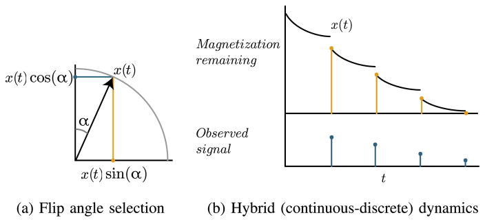
We acquire data at N time points separated by intervals of length T_R. Each time t an acquisition is made, we must choose a flip angle α_k,t for each compound k to be measured. If the magnetization of the k-th compound before the acquisition is x_k, then this choice of flip angle allows us to measure a signal of magnitude sin(α_k,t)x_k, after which cos(α_k,t)x_k magnetization remains for future acquisitions (Fig. 1a). This causes discrete jumps, or resets, in the system state, leading to a hybrid dynamical system [14] (Fig. 1b). Since we are only interested in the system’s state at acquisition times, we can avoid technicalities associated with hybrid system modelling by discretizing the system in time and considering a discrete-time dynamical system that simultaneously captures the evolution of (1) between acquisitions and the discrete jumps induced by the acquisitions. We define the transition matrices A_d and B_d

Fig. 1.

Illustration of the trade-off between present and future image intensity in a single compound. (a) Each acquisition relies on choosing an angle α to perturb the longitudinal magnetization into the transverse plane, allowing a measurement of magnitude x(t) sin(α), after which x(t) cos(α) longitudinal magnetization remains for future acquisitions. (b) Repeated excitation leads to repeated discrete jumps in the system state, depleting the remaining magnetization.

$$\begin{array}{ll}{A}_d\hfill & =exp\left(T_R\left[\begin{array}{cc}-k_{PL}-R_{1P}& 0\\ k_{PL}& -R_{1L}\end{array}\right]\right)\hfill \\ B_d\hfill & ={\left[\begin{array}{cc}-k_{PL}-R_{1P}& 0\\ k_{PL}& -R_{1L}\end{array}\right]}^{-1}(A_d-I)\left[\begin{array}{c}{k}_{\mathit{TRANS}}\\ 0\end{array}\right]\hfill \end{array}$$

that correspond to the discretization of (1) assuming a zero-order hold on the input between each acquisition [15].

We will construct metabolite maps using magnitude image data, which necessitates a Rician noise model. Using magnitude images allows us to avoid modelling sources of phase in the image which would require additional states and parameters to estimate. It would also be possible to perform the parameter mapping using complex images with Gaussian noise, but this would require revising the model to account for phase, or modifying the image reconstruction to estimate and remove phase from the acquired images.

Accordingly, we model the measurements as independent Rician-distributed random variables [16], which have probability density

$$p_{x,\sigma }(y)=\frac{y}{{\sigma }^2}exp\left(-\frac{y^2+x^2}{2{\sigma }^2}\right)I_0\left(\frac{yx}{{\sigma }^2}\right)$$

where I_ν denotes the modified Bessel function of the first kind of order ν. All together, we have the discrete-time model

$$\begin{array}{ll}\hfill x_0& =0\hfill \\ \hfill x_{t+1}& =A_d(\theta )\left[\begin{array}{cc}cos{\alpha }_{1,t}& 0\\ 0& cos{\alpha }_{2,t}\end{array}\right]x_t+B_d(\theta )u_t(\theta )\hfill \\ \hfill {\stackrel{\sim }{x}}_{k,t}& =sin({\alpha }_{k,t})x_{k,t}k=1,2\hfill \\ \hfill Y_{k,t}& ~\mathit{Rice}({\stackrel{\sim }{x}}_{k,t},{\sigma }_k)k=1,2.\hfill \end{array}$$ (2)

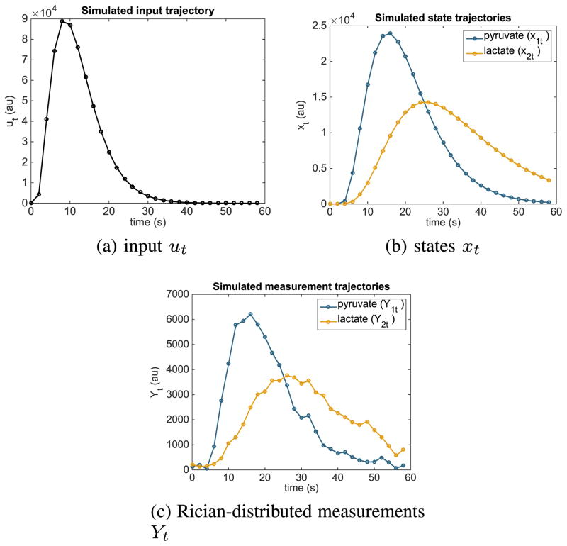
Simulated trajectories of this model are shown in Fig. 2.

Fig. 2.

Simulated trajectories of the model (2) using a constant flip angle sequence with α_k,t = 15°.

The model parameters are

$$\theta =[R_{1P},R_{1L},k_{PL},k_{\mathit{TRANS}},u_0,\dots ,u_{N-1}]$$

and we have the freedom to choose

$$\alpha =\left[\begin{array}{ccc}{\alpha }_{1,1}& \dots & {\alpha }_{1,N}\\ {\alpha }_{2,1}& \dots & {\alpha }_{2,N}\end{array}\right]$$

to generate the best possible estimate of the unknown parameters. The noise parameters σ_k for k = 1, 2 can be estimated separately from a measurement of the background and are therefore assumed to be known. We fix a sampling interval of T_R = 2 seconds, though this could in principle be included as a decision variable.

III. Optimal Experiment Design

In this section, we present a methodology for designing flip angle sequences to provide maximal information about the metabolic rate parameter k_PL. This methodology is based on an optimization problem that can be solved to local optimality using nonlinear programming. To facilitate the implementation of this methodology, we have released an open source MAT-LAB toolbox for the design of optimal flip angle sequences. This toolbox is available at https://github.com/maidens/Flip-Angle-Design-Toolbox.

A. Theory

The goal of optimal experiment design is to estimate parameters in a statistical model from observed data with minimum variance in the estimates [17]. The most commonly used optimization criteria are scalar-valued functions of the Fisher information matrix. For a statistical model described by a family of probability density functions p_θ(y) parametrized by a vector of parameters θ ∈ ℝ^p, the Fisher information is a p × p symmetric, positive semidefinite matrix defined as

$${\mathcal{I}}_{ij}(\theta )=\mathbb{E}\left[\frac{\partial log{p}_{\theta }(Y)}{\partial {\theta }_i}\frac{\partial log{p}_{\theta }(Y)}{\partial {\theta }_j}\right]$$

where the expectation is computed under the distribution p_θ.

In linear regression models with Gaussian-distributed measurements, the maximum-likelihood estimator of θ is unbiased and has covariance equal to the inverse of the Fisher information matrix. Thus the variance of estimates of θ can be minimized by maximizing the Fisher information. For general models, the Cramér-Rao inequality

$$cov(\widehat{\theta })\ge {\mathcal{I}}^{-1}$$ (3)

gives a lower bound on the covariance of any unbiased estimator θ̂ of the parameter θ in terms of the Fisher information matrix. In general, finite-sample efficient estimators do not exist, that is, there is no estimator that can achieve the Cramér-Rao bound based on a single experiment, or even a finite number of independent experiments. Nonetheless, the Fisher information is commonly used in optimal experiment design in nonlinear models as it is general, easy to compute, provides good results in practice and can be justified mathematically via asymptotic analysis [18].

In this paper, we will estimate unknown model parameters using the maximum likelihood estimator (MLE) defined as

$${\widehat{\theta }}_{\mathit{MLE}}\in arg\underset{\theta \in {ℝ}^p}{max}{p}_{\theta }(Y)$$

where Y is the observed data. Under mild assumptions, the maximum likelihood estimator is asymptotically efficient [19], that is,

$$\sqrt{n}({\widehat{\theta }}_{\mathit{MLE}}-\theta )\stackrel{d}{\to }\mathcal{N}(0,{\mathcal{I}}^{-1})$$ (4)

as the number n of independent data sets used to compute the MLE tends to infinity. Here 𝒩(0, ℐ⁻¹) denotes the multivariate normal distribution with mean zero and covariance ℐ⁻¹ and $\stackrel{d}{\to }$ denotes convergence in distribution. Thus, we see that asymptotically the MLE achieves the Cramér-Rao bound. While it is not necessarily the case in general that the MLE based on a single data set, or any finite number of data sets, has covariance equal to ℐ⁻¹, it is often a good approximation. Thus, we attempt to design an experiment to reliably estimate θ by maximizing the Fisher information.

The Fisher information is a function of the true value of the parameter vector θ, which is unknown a priori. There are commonly three approaches to overcome this difficulty:

1. Minimax/maximin optimal design: Given a range Θ of values for the parameter vector choose the design α to maximize the worst-case information among all potential values of the parameter θ ∈ Θ (i.e. α^* = arg max_α∈𝒜 min_θ∈Θ μ(ℐ(θ, α)) for some measure μ of the size of the information matrix). This approach is advantageous because it provides a guaranteed lower bound on the information gained from an experiment despite parametric uncertainty. But it typically leads to a design α^* that is optimized for a “corner case” in the parameter space, which may be overly conservative in practice. In addition, minimax/maximin objective functions are non-differentiable and can be difficult to optimize numerically [20], [21].

2. Bayesian optimal design: Given a prior distribution p₀(θ) on the space of possible parameter values, maximize the expected information (i.e. α^* = arg max_α∈𝒜 ∫ μ(ℐ(θ, α)) p₀(θ)dθ). This approach handles parametric uncertainty nicely, but can lead to difficulties when it in unclear how to choose an appropriate prior, or when the parameter space is large and hence the computation of the high-dimensional integral is numerically intractable [22].

3. Choose a nominal value θ₀ of the parameter vector at which to optimize the information (i.e. α^* = arg max_α∈𝒜 μ(ℐ(α, θ₀))). This approach is conceptually simple and numerically tractable, but may suffer from a lack of robustness to the choice of θ₀.

In this paper, we take the third approach. We address the potential lack of robustness to the choice of the nominal parameter value θ₀ by a systematic numerical study of the robustness to parametric uncertainty in Section IV-C. These experiments demonstrate that for this particular model, an experiment designed using nominal values of the model parameters performs well across a wide range of values of the true parameter. It is possible that the results presented here could be improved further based on a minimax or Bayesian formulation, but this investigation is beyond the scope of this paper.

B. Computing Fisher information for our model

To find a maximum-likelihood estimate with minimum variance, we choose the sequence α to maximize the Fisher information matrix at a nominal value of the parameter vector θ. The nominal parameter values used are given in Table I. The T₁ relaxation, perfusion and metabolic rate parameters were chosen based on our typical data in a prostate cancer mouse model, and nominal values for the input shape and noise parameters were chosen based on a maximum likelihood fit to an arterial input function measured in a preliminary experiment.

To compute the Fisher information, we use the expression derived in [23] for the (i, j)-th entry of ℐ:

$${\mathcal{I}}_{ij}=\sum _{t=0}^N\sum _{k=1}^2\frac{1}{{\sigma }_k^2}\frac{\partial {\stackrel{\sim }{x}}_{k,t}}{\partial {\theta }_i}\frac{\partial {\stackrel{\sim }{x}}_{k,t}}{\partial {\theta }_j}\psi \left(\frac{{\stackrel{\sim }{x}}_{k,t}}{{\sigma }_k}\right)$$ (5)

where the sensitivities are computed recursively as

$$\{\begin{array}{l}\frac{\partial x_0}{\partial {\theta }_i}=0\hfill \\ \frac{\partial x_{t+1}}{\partial {\theta }_i}=\frac{\partial A_d}{\partial {\theta }_i}\left[\begin{array}{cc}cos{\alpha }_{1,t}& 0\\ 0& cos{\alpha }_{2,t}\end{array}\right]x_t+A_d\left[\begin{array}{cc}cos{\alpha }_{1,t}& 0\\ 0& cos{\alpha }_{2,t}\end{array}\right]\frac{\partial x_t}{\partial {\theta }_i}+\frac{\partial B_d}{\partial {\theta }_i}{u}_t+B_d\frac{\partial u_t}{\partial {\theta }_i}\hfill \\ \frac{\partial {\stackrel{\sim }{x}}_t}{\partial {\theta }_i}=\left[\begin{array}{cc}sin{\alpha }_{1,t}& 0\\ 0& sin{\alpha }_{2,t}\end{array}\right]\frac{\partial x_t}{\partial {\theta }_i}\hfill \end{array}$$

and ψ is defined in terms of the integral

$$\psi (z)=-z^2+{\int }_0^{\infty }{y}^3\frac{I_1^2(yz)}{I_0(yz)}exp\left(-\frac{1}{2}(y^2+z^2)\right)dy.$$

C. Eliminating nuisance parameters

In practice, we do not necessarily need good estimates of all the unknown parameters in the model. For example, in this paper our primary goal is to estimate the metabolic rate parameter k_PL which is useful for discriminating between cancerous and non-cancerous tissues [5], determining the severity of disease [24], [25] and monitoring response to therapy [2]. Thus we wish to modify our optimality criterion to maximize the sensitivity of the experiments to k_PL while considering the nuisance parameters only insofar as they allow us to estimate the parameters of interest. We do so by partitioning the information matrix as

$$\mathcal{I}=\left[\begin{array}{cc}{\mathcal{I}}_{11}& {\mathcal{I}}_{12}\\ {\mathcal{I}}_{21}& {\mathcal{I}}_{22}\end{array}\right]$$

where the first block corresponds to the parameters of interest and the second block corresponds to the nuisance parameters. The inverse of the Fisher information is given by

$${\mathcal{I}}^{-1}=\left[\begin{array}{cc}{({\mathcal{I}}_{11}-{\mathcal{I}}_{12}{\mathcal{I}}_{22}^{-1}{\mathcal{I}}_{21})}^{-1}& -{\mathcal{I}}_{11}^{-1}{\mathcal{I}}_{12}{({\mathcal{I}}_{22}-{\mathcal{I}}_{21}{\mathcal{I}}_{11}^{-1}{\mathcal{I}}_{12})}^{-1}\\ -{\mathcal{I}}_{22}^{-1}{\mathcal{I}}_{21}{({\mathcal{I}}_{11}-{\mathcal{I}}_{12}{\mathcal{I}}_{22}^{-1}{\mathcal{I}}_{21})}^{-1}& {({\mathcal{I}}_{22}-{\mathcal{I}}_{21}{\mathcal{I}}_{11}^{-1}{\mathcal{I}}_{12})}^{-1}\end{array}\right].$$

Thus, optimal design for the parameters of interest can be performed by maximizing the Schur complement of ℐ₂₂:

$$\mathcal{S}={\mathcal{I}}_{11}-{\mathcal{I}}_{12}{\mathcal{I}}_{22}^{-1}{\mathcal{I}}_{21}$$

which corresponds to minimizing the asymptotic covariance of the marginal distribution of the MLE corresponding to the parameters of interest via (4), or equivalently, minimizing the Cramér-Rao bound on the parameters of interest via (3).

In general, if multiple parameters are of interest then 𝒮 will be a matrix and we would be required to choose a suitable scalar criterion for measuring the size of 𝒮. The problem of simultaneously estimating k_PL and k_TRANS is considered in [23], where the D–, E– and A– optimality criteria are compared. However, in this instance we are considering a single parameter of interest k_PL, therefore the Schur complement 𝒮 is scalar-valued.

D. Regularization

We desire a smoothly-varying sequence of flip angles for a number of reasons including increasing robustness against model mismatch and interpretability of the resulting sequence of flip angles. We achieve smoothness in the flip angle sequence by adding a regularization term λ||Δα||_F to the objective function to penalize nonsmooth sequences where the differencing operator Δ is defined as

$$\mathrm{\Delta }\left(\left[\begin{array}{ccc}{\alpha }_{1,1}& \dots & {\alpha }_{1,N}\\ {\alpha }_{2,1}& \dots & {\alpha }_{2,N}\end{array}\right]\right)=\left[\begin{array}{ccc}({\alpha }_{1,2})-{\alpha }_{1,1}& \dots & ({\alpha }_{1,N}-{\alpha }_{1,N-1})\\ ({\alpha }_{2,2}-{\alpha }_{2,1})& \dots & ({\alpha }_{2,N}-{\alpha }_{2,N-1})\end{array}\right]$$

and ||·||_F denotes the Frobenius norm. The nonnegative parameter λ can be adjusted to achieve the desired degree of smoothness.

Regularization also improves the convexity of the objective function. When the regularization parameter takes the value λ = 0, the objective function possesses multiple local minima, but as λ → ∞ the convex term ||Δα||_F dominates, which guarantees that any stationary point is a global optimum.

We chose a particular value of λ by comparing the flip angle sequences resulting from the optimization using numerous regularization parameter values. The value λ = 0.1 was found to nicely balance between smoothness and range (between 0° and 90°) of the flip angle sequence.

E. Numerical optimization

To design an optimal flip angle scheme, we must solve the flip angle optimization problem

$$\begin{array}{ll}\text{maximize}\hfill & \mathcal{S}(\theta ,\alpha )-\lambda {\Vert \mathrm{\Delta }\alpha \Vert }_F\hfill \\ \text{subject}\text{to}\hfill & 0°\le {\alpha }_{k,t}\le 90°k=1,2t=1,\dots ,N\hfill \end{array}$$ (6)

for the flip angle sequence α where θ is fixed to some nominal value for the unknown parameters. The MATLAB Optimization Toolbox [26] provides a derivative-free implementation of the quasi-Newton optimization algorithm of Broyden-Fletcher-Goldfarb-Shanno (BFGS) [27], which is well-suited to finding local optima of this objective function.

F. Results

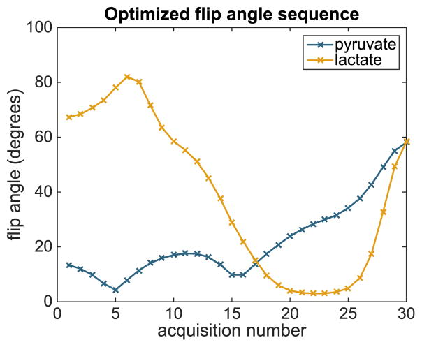
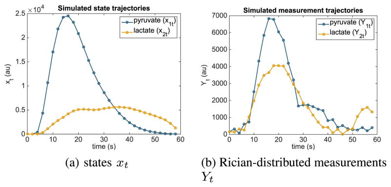
A solution to the optimization problem (6), initialized at α_k,t = 5°, is given in Fig. 3. Simulated state and observation trajectories corresponding to this flip angle sequence are shown in Fig. 4.

Fig. 3.

Optimized flip angle sequence for estimating the metabolic rate parameter k_PL using the nominal parameter values in Table I and a sampling interval T_R = 2 s between acquisitions.

Fig. 4.

Simulated trajectories of the model (2) using the optimized flip angle sequence shown in Fig. 3 and the arterial input function shown in Fig. 2a.

We see that the pyruvate flip angles follow a pattern similar to flip angle sequences designed for other objectives, beginning with small flip angles to preserve magnetization for future acquisitions but increasing toward the end of the sequence [9], [10]. In contrast, the optimized flip angle sequence is much more aggressive with the lactate flip angles at the beginning of the experiment than in other variable flip angle sequences. This provides more reliable information about the leading end of the lactate time series, which contains the most information about the metabolic rate.

For the particular model and regularization parameter values used, the BFGS optimization algorithm converges to the same optimal sequence for a wide range of initializations. To confirm this, we have initialized the search algorithm using three flip angle sequences with angles generated randomly between 0 and 90°. For all three initializations, the algorithm converges to the flip angle sequence shown in Fig. 3. This demonstrates that the flip angle sequence presented is likely a global optimum.

IV. Validation Using Simulated Data

In this section, we demonstrate the advantage of the optimally designed flip angle sequence using computer-simulated data. Working with simulated data allows us to collect a large number of statistically independent data sets and provides us access to a “ground truth” value for the parameter vector. This makes it possible to reliably determine the parameter estimation error that results from noise in the simulated measurements. It is not feasible to acquire such a large number of data sets in vivo, and these would also not include ground truth values. Thus we use simulated data to demonstrate that our optimized flip angle sequence leads to smaller uncertainty in estimates of the metabolic rate parameter k_PL.

A. Two-step parameter estimation procedure

When fitting the data from in vivo experiments, data from different voxels will correspond to different values of the parameters k_TRANS, k_PL, R_1P and R_1L as these values change with spatial location, but all correspond to the same arterial input u(t). Thus we present a fitting procedure that proceeds in two steps: first we fit a single input function u(t) to the entire data set, then we fix this input function and estimate values of the remaining parameters individually for each of the voxels in the slice.

B. Simulation results and discussion

We wish to compare the reliability of estimates of k_PL between data generated using five competing flip angle sequences:

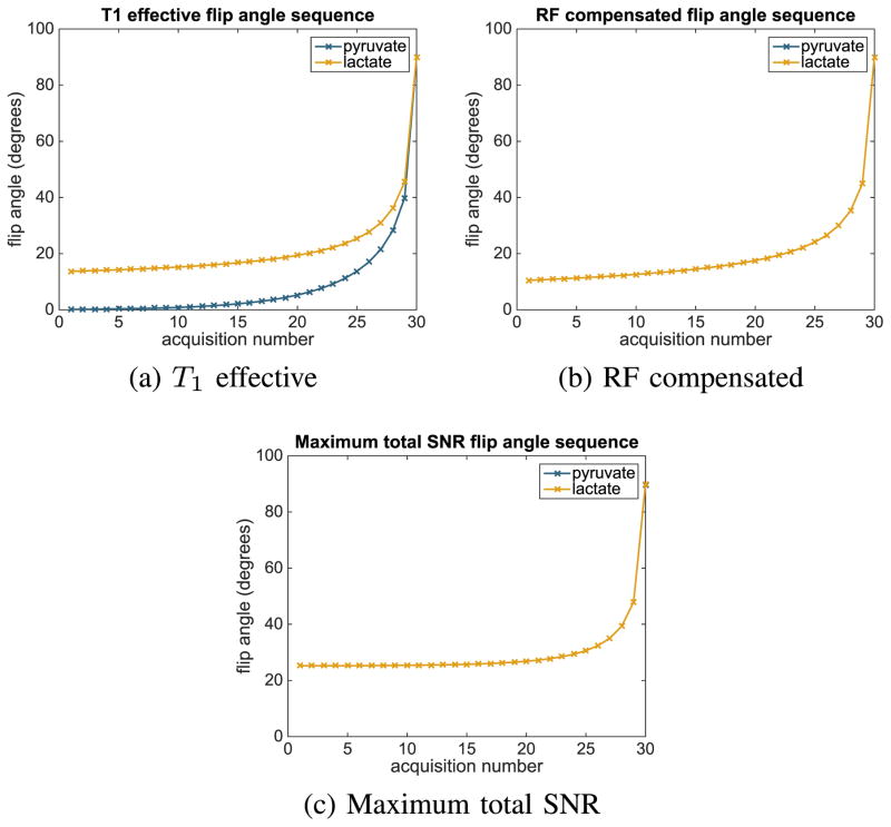
1. a T₁-effective sequence [9] that aims to keep the measured signal constant despite repeated RF excitation and magnetization exchange between chemical compounds (Fig. 5a)

2. an RF compensated flip angle sequence [28] that aims to keep the measured signal constant despite repeated RF excitation (Fig. 5b),

3. a constant flip angle sequence of 15°,

4. a sequence that maximizes the total signal-to-noise ratio in the observed signal

   $${\mathit{SNR}}_{\mathit{total}}=\sum _{t=0}^N\sum _{k=1}^2\frac{{\stackrel{\sim }{x}}_{k,t}}{{\sigma }_k}.$$

   [10] (Fig. 5b), and

5. our flip angle sequence that maximizes the Fisher information about k_PL (Fig. 3).

Fig. 5.

Flip angle schedules compared experimentally with our optimized flip angle sequence. Note that for the RF compensated and maximum total SNR schedules, the sequences corresponding to pyruvate and lactate are identical.

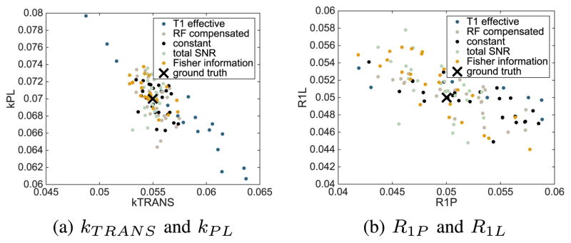
For each of the five flip angle sequences, we simulate n = 25 independent data sets from the model (2) using the parameter values given in Table I. We then perform the two-step parameter estimation procedure described in Section IV-A. The resulting parameter estimates are shown in Fig. 6. We see that for all five flip angle sequences, the parameter estimates congregate near the ground truth value of the model parameters.

Fig. 6.

Maximum likelihood estimates of the parameters k_TRANS, k_PL, R_1P and R_1L for numerous independent simulated data sets compared between five flip angle sequences for σ² = 2.3608 × 10⁴. The ground truth value is depicted as ×.

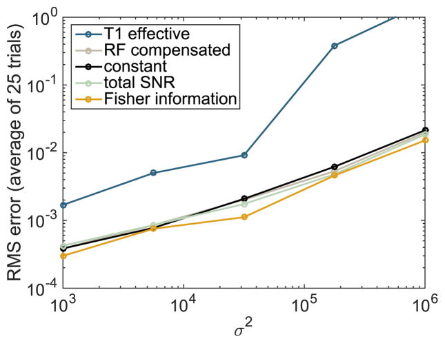
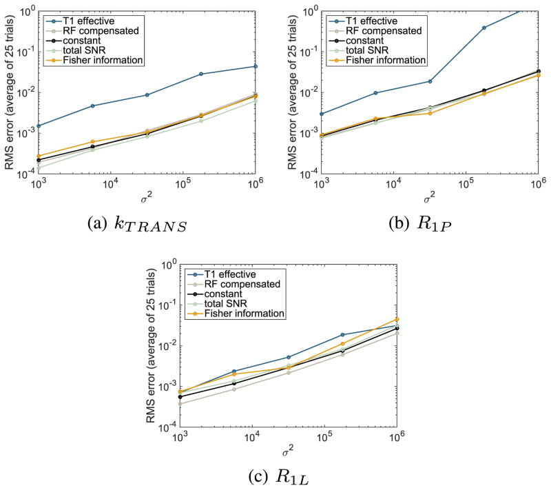
To demonstrate that our optimized flip angle sequence provides more accurate estimates of k_PL than the competing flip angle sequences, we compare the root mean squared (RMS) estimation error between the sequences. We repeat this experiment for various values of the noise parameter σ² ranging from 10³ to 10⁶ to demonstrate that the improvement in the estimates is robust to variation in the noise strength. A value of approximately 2 × 10⁴, in the center of this range, is typical for prostate tumor mouse model experiments. For each value of σ ² we compute the RMS error of the k_PL and nuisance parameter estimates across the n = 25 trajectories and plot these relationships in Figs. 7 and 8 respectively. The average improvement compared with competing sequences, across a range of noise parameter values {σ_p, p = 1,..., 5}, is computed as a percentage

Fig. 7.

Comparison of the root mean square k_PL estimation error between various flip angle sequences across different values of the noise strength parameter σ².

Fig. 8.

Comparison of the root mean square nuisance parameter estimation error between various flip angle sequences across different values of the noise strength parameter σ².

$$100\times \left(\frac{1}{5}\sum _{p=1}^5\left[1-\frac{{\mathit{RMS}}_{\mathit{Fisher}}({\sigma }_p)}{{\mathit{RMS}}_{\mathit{competing}}({\sigma }_p)}\right]\right).$$

These improvement percentages are summarized in Table II.

TABLE II.

Improvement in metabolic rate estimate achieved by Fisher information sequence against competing sequences

Competing sequence	T1 effective	RF compensated	Constant 15°	total SNR
Improvement achieved	90.6%	23.1%	25.3%	19.8%

Overall, we see that the optimized flip angle sequence provides a more reliable estimate of the parameter of interest k_PL, with a substantial improvement over all four competing flip angle schedules. The magnitude of the improvement varies from a 91% decrease in the estimation error against the T₁ effective sequence to a 20% decrease compared against the closest competitor: the maximum total SNR sequence. This improvement comes at the expense of less reliable estimates of some of the nuisance parameters. This highlights the advantage of using optimization-based methods to manage trade-offs in experiment design.

C. Robustness to parametric uncertainty

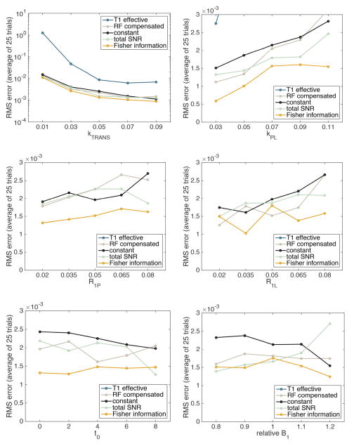
Based on the simulation experiments described in Section IV-B we have argued that flip angles optimized based on the Fisher information lead to smaller error in estimates of the parameter of interest k_PL when the same parameter values are used for the simulation and flip angle optimization. In this section we dispense with the latter assumption to demonstrate that this improvement is robust to uncertainty in the model parameters. We use the flip angle sequence shown in Fig. 3, which was designed using the specific model parameters given in Table I, along with two competing flip angle sequences to simulate data from models with different values for the parameters k_TRANS, k_PL, R_1P, R_1L and t₀ as well as a factor ΔB₁ multiplying the flip angle sequence, used to demonstrate robustness to known B₁ inhomogeneities.

The ranges of the varying parameters were chosen to represent realistic physiological ranges and to center near the values we typically observe in a prostate tumor (TRAMP) mouse model. In Fig. 9 we plot the ensemble RMS error over n=25 simulated data sets as a function of the model parameter modified in the simulated data.

Fig. 9.

Simulated comparison of the k_PL estimation error across values of the model parameters. The error is compared between five flip angle sequences shown in Figs. 3 and 5. These flip angle sequences are computed based on the nominal values of the model parameters given in Table I and held fixed across all comparisons. Note that the first graph is logarithmically scaled, due to the fact that low perfusion leads to significant uncertainty in the metabolic rate estimates. Some estimation errors corresponding to the T₁ effective sequence are greater than the maximum value plotted on these axes.

We see that the flip angles optimized based on Fisher information lead to better estimates of k_PL across nearly the entire range of model parameters used, despite no longer being optimal for the parameter values used to generate the data. This provides strong evidence that not exactly knowing the parameter values a priori does not limit the usefulness of our proposed flip angle design methodology.

V. In Vivo Experiments

We now move on to in vivo experiments. In contrast with the in silico experiments, here there is no ground truth value of the model parameters against which to compare our estimates, as the true rates are unknown and may vary between different regions of the tissue. However, the in vivo experiments can be used to show well-foundedness of the model that we have chosen and to demonstrate the feasibility of model-based parameter mapping using our optimized time-varying flip angle sequence. We show that our model can reliably reproduce observed data and achieve consistent parameter estimates across a variety of time-varying flip angle sequences.

A. Experimental setup

To implement this technique in vivo, metabolic data were acquired in a prostate tumor mouse (TRAMP) model using a 3T MRI scanner (MR750, GE Healthcare). Briefly, 24μL aliquots of [1-¹³C] pyruvic acid doped with 15mM Trityl radical (Ox063, GE Healthcare) and 1.5mM Dotarem (Guerbet, France) were inserted into a Hypersense polarizer (Oxford Instruments, Abingdon, England) and polarized for 60 minutes. The sample was then rapidly dissoluted with 4.5g of 80mM NaOH/40mM Tris buffer to rapidly thaw and neutralize the sample. Following dissolution, 450μL of 80mM pyruvate was injected via the tail vein over 15 seconds, and data acquisition coincided with the start of injection. Metabolites from a single slice were individually excited with a singleband spectral-spatial RF pulse and encoded with a single-shot symmetric EPI readout [29], with a repetition time of 100ms, a field-of-view of 53 × 53mm, a matrix size of 16 × 16, an 8mm slice thickness, and a 2 second sampling interval. A ¹H image showing the anatomy contained in the slice in question is given in Fig. 10.

Fig. 10.

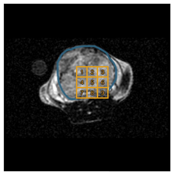
¹H image of the slice of interest. A large tumor, outlined in blue, fills a significant portion of the slice. Numbered volumes used to extract trajectories for parameter estimation are outlined in gold.

Datasets were acquired using three time-varying flip angle sequences. The T₁-effective and RF-compensated sequences, shown in Figs. 5a and 5b respectively, aim to distribute observed magnetization evenly across acquisitions, leading to roughly constant observed signals over time. The RF-compensated sequence does so by accounting for magnetization lost due to repeated RF excitation, but ignoring exchange between chemical compounds and T₁ relaxation [28]. In contrast, the T₁-effective sequence accounts for exchange and T₁ relaxation as well as RF excitation in attempting to achieve a flat time profile [9]. We compare these two sequences against our sequence, shown in Fig. 3, that has been optimized with respect to the Fisher information about k_PL.

B. Resulting data

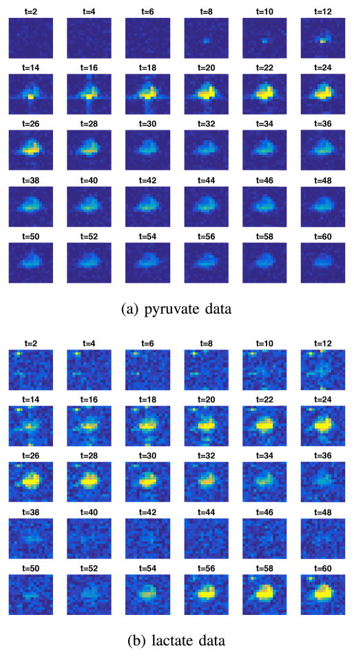
An example of the collected data, from the experiment with the Fisher information-optimized flip angles, is shown in Fig. 11. Experimentally-estimated values for the noise parameters are given in Table III.

Fig. 11.

Data collected using the optimized flip angles shown in Fig. 3. The field-of-view of these images is identical to the ¹H image in Fig. 10.

TABLE III.

Maximum-likelihood estimates of the noise parameter ${\sigma }_k^2$ For each of the three data sets collected

	T1 effective	RF compensated	Fisher information
${\sigma }_1^2$ (pyruvate)	1.84 × 104	2.05 × 104	2.21 × 104
${\sigma }_2^2$ (lactate)	2.14 × 104	1.97 × 104	3.26 × 104

C. Flip angle profile modelling

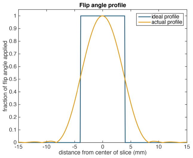
Due to an imperfect (non-rectangular) slice profile, flip angles applied in practice vary spatially across the slice. This can lead to excess signal coming from regions near the boundary of the slice at later time points in the acquisitions, a phenomenon known as the slice profile effect [30], [31]. We have found that it is necessary to account for this effect in order to accurately fit the experimental data.

We consider the actual slice profile π(z) shown in Fig. 12 which corresponds to the spatial response of the RF pulse used experimentally. We assume that at each time step t and for each compound k (i.e. k = 1 corresponding to pyruvate, k = 2 corresponding to lactate) we can choose a real parameter α_k,t such that the flip angle applied at location z is θ_k,t(z) = α_k,t π(z). To generate a finite-dimensional model of the dynamics, we consider the magnetization dynamics at a discrete set of z coordinates {z₁,..., z_N}. The magnetization at location z_i in the slice is then governed by the equations

Fig. 12.

Comparison between an ideal flip angle profile across the slice and the actual profile for the RF excitation pulse used.

$$x_{i,t+1}=A_d\left[\begin{array}{cc}cos({\alpha }_{1,t}\pi (z_i))& 0\\ 0& cos({\alpha }_{2,t}\pi (z_i))\end{array}\right]x_{i,t}+B_d{u}_t(p)$$

and the total magnetization measured is then assumed to be distributed

$$\begin{array}{ll}\hfill {\stackrel{\sim }{x}}_t& =\sum _{i=1}^N\frac{1}{z_{i+1}-z_i}\left[\begin{array}{cc}sin({\alpha }_{1,t}\pi (z_i))& 0\\ 0& sin({\alpha }_{2,t}\pi (z_i))\end{array}\right]x_{i,t}\hfill \\ \hfill Y_{k,t}& ~\mathit{Rice}({\stackrel{\sim }{x}}_{k,t},{\sigma }^2).\hfill \end{array}$$

This approach accounts for the slice profile effects by modelling the dynamics across the actual slice profile.

D. Parameter estimation

We begin by extracting time evolutions of the measured pyruvate and lactate signal from n = 9 voxels in the slice. The chosen volumes from which these signals are extracted are illustrated in Fig. 10. As in Section IV, parameter estimation is performed in two steps. First, a single arterial input function and value for the parameter R_1L are estimated based on the spatial average of the time series extracted from the tumor region. Second, the estimated input function and R_1L value are held fixed while model parameters k_TRANS and k_PL are fit individually to the time series extracted from each of the voxels. To ensure practical identifiability of the model, the parameter R_1P is fixed to a value of 0.05 during both steps.

E. In vivo results and discussion

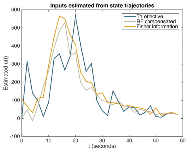
Estimates of the arterial input corresponding to each of the three flip angle sequences are shown in Fig. 13. We see that the estimated inputs are reasonably consistent between the three data sets, but have some variation due to measurement noise in the pyruvate signal. Our optimized sequence yields the most smoothly-varying input function, which suggests that it is likely the most reliable of the three estimated AIFs.

Fig. 13.

Estimated arterial input functions corresponding to each of the three flip angle sequences given in Figs. 3 and 5.

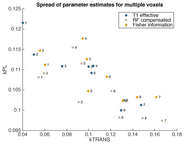
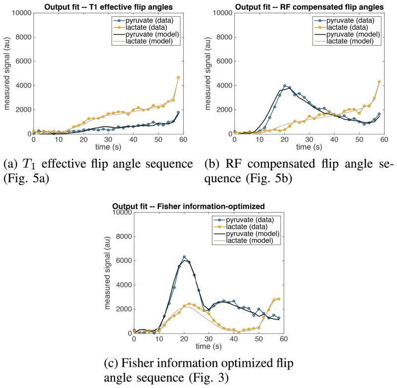
Parameter estimates corresponding to each of the nine voxels are compared between the three flip angle sequences in Fig. 14. Examples of the quality of the fit corresponding to a particular voxel are shown in Fig. 15. We see that the estimated parameter values are consistent between the three flip angle sequences and that our model is able to reliably reproduce the observed data in all three cases. This provides evidence that the model we have used in this paper accurately describes the dynamics of magnetization exchange in vivo, and hence that the decision to use this model for the numerical reliability experiments of Section IV is well-founded.

Fig. 14.

Maximum likelihood estimates of the parameters k_TRANS and k_PL for time series trajectories extracted from various voxels, labelled 1 through 9. The resulting estimates are compared between data sets collected using the three flip angle sequences shown in Figs. 3 and 5.

Fig. 15.

Model fit to a collection of experimentally measured time series data corresponding to voxel number 5. Each of the three data sets was collected using a different flip angle sequence.

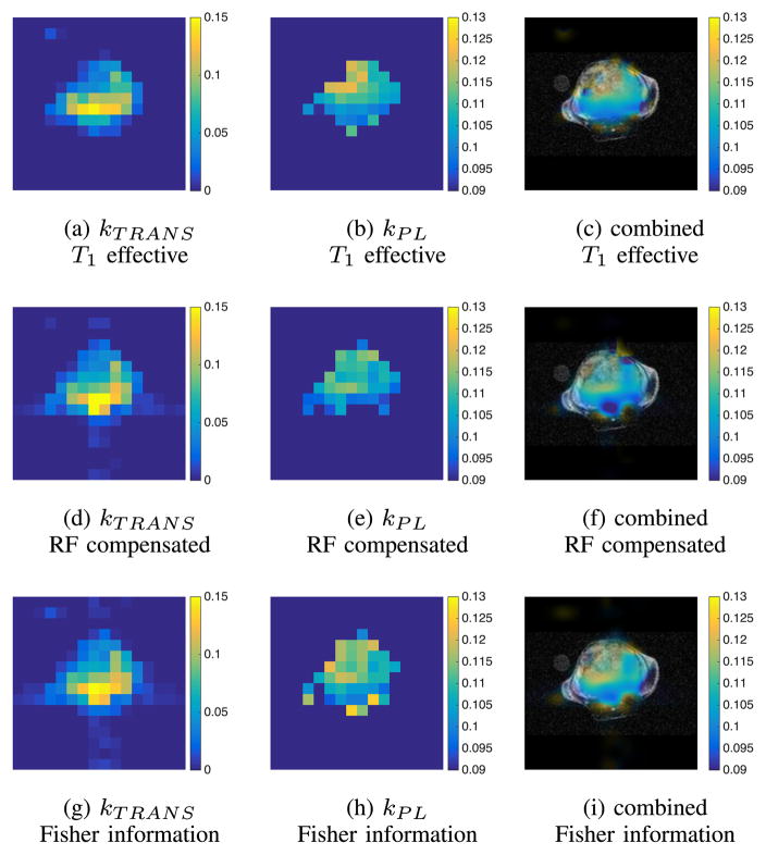
We also present maps that show the spatial distribution of estimated metabolic and perfusion rates in Fig. 16. We see that the range and spatial distribution of parameter estimates are consistent between acquisition sequences.

Fig. 16.

Maps of the perfusion rate parameter k_TRANS and metabolic rate parameter k_PL corresponding to each of the three flip angle sequences. The k_PL maps are masked outside the perfused region using a threshold of k_TRANS = 0.02. A single map combining anatomic, perfusion and metabolism information is shown on the right. In this map, the color is determined by the estimated k_PL value while the transparency of the map is set using the perfusion rate parameter k_TRANS such that in highly-perfused tissues where the estimates of the metabolic rate parameter are more reliable the map is less transparent. The combined image data are zero-filled from 16 × 16 to 256 × 256 to match the resolution of the ¹H images.

VI. Conclusion

We have presented a method of generating optimal flip angle sequences for estimating the metabolic rate in a model of pyruvate metabolism. This method uses the Fisher information about the parameter of interest as the objective function that we wish to maximize. We have shown that the resulting flip angle sequence leads to smaller variance in the parameter estimates due to noise in the measured signal. We have demonstrated this in silico where we can explicitly compare the estimated model parameter values against the ground truth value. In this simulation experiment we demonstrated that our flip angle sequence leads to a 20% to 90% decrease in the uncertainty of the estimated metabolic rate, when compared with existing sequences. We also performed in vivo experiments to provide evidence that the model used in the in silico experiments is well-founded and demonstrate the feasibility of metabolic rate estimation and parameter mapping using this novel sequence. Based on the reliability results demonstrated in silico and the in vivo experiments demonstrating the appropriateness of the model used for the in silico experiments we argue that, for experiments that aim to quantitatively compare metabolic rates, optimizing flip angle sequences based on the Fisher information will probably lead to more reliable estimates of the model parameters of interest.

References

- 1.Golman K, Petersson SJ. Metabolic imaging and other applications of hyperpolarized 13C1. Academic Radiology. 2006 Aug;13(8):932–942. doi: 10.1016/j.acra.2006.06.001. [DOI] [PubMed] [Google Scholar]
- 2.Day SE, Kettunen MI, Gallagher FA, Hu D-E, Lerche M, Wolber J, Golman K, Ardenkjær-Larsen JH, Brindle KM. Detecting tumor response to treatment using hyperpolarized 13C magnetic resonance imaging and spectroscopy. Nature Medicine. 2007;11:1382–1387. doi: 10.1038/nm1650. [DOI] [PubMed] [Google Scholar]
- 3.Kazan SM, Reynolds S, Kennerley A, Wholey E, Bluff JE, Berwick J, Cunningham VJ, Paley MN, Tozer GM. Kinetic modeling of hyperpolarized 13C pyruvate metabolism in tumors using a measured arterial input function. Magnetic Resonance in Medicine. 2013;70(4):943–953. doi: 10.1002/mrm.24546. [DOI] [PubMed] [Google Scholar]
- 4.Nelson SJ, Kurhanewicz J, Vigneron DB, Larson PEZ, Harzstark AL, Ferrone M, van Criekinge M, Chang JW, Bok R, Park I, Reed G, Carvajal L, Small EJ, Munster P, Weinberg VK, Ardenkjær-Larsen JH, Chen AP, Hurd RE, Odegardstuen LI, Robb FJ, Tropp J, Murray JA. Metabolic imaging of patients with prostate cancer using hyperpolarized [1-13C]pyruvate. Science Translational Medicine. 2013;5(198):198ra108. doi: 10.1126/scitranslmed.3006070. [DOI] [PMC free article] [PubMed] [Google Scholar]
- 5.Bahrami N, Swisher CL, von Morze C, Vigneron DB, Larson PEZ. Kinetic and perfusion modeling of hyperpolarized 13C pyruvate and urea in cancer with arbitrary RF flip angles. Quantitative Imaging in Medicine and Surgery. 4(1):2014. doi: 10.3978/j.issn.2223-4292.2014.02.02. [DOI] [PMC free article] [PubMed] [Google Scholar]
- 6.Swisher CL, Larson PEZ, Kruttwig K, Kerr AB, Hu S, Bok RA, Goga A, Pauly JM, Nelson SJ, Kurhanewicz J, Vigneron DB. Quantitative measurement of cancer metabolism using stimulated echo hyperpolarized carbon-13 MRS. Magnetic Resonance in Medicine. 2014;71(1):1–11. doi: 10.1002/mrm.24634. [DOI] [PMC free article] [PubMed] [Google Scholar]
- 7.Ardenkjær-Larsen JH, Fridlund B, Gram A, Hansson G, Hansson L, Lerche MH, Servin R, Thaning M, Golman K. Increase in signal-to-noise ratio of > 10,000 times in liquid-state NMR. Proceedings of the National Academy of Sciences. 2003 Sep;100(18):10 158–10 163. doi: 10.1073/pnas.1733835100. [DOI] [PMC free article] [PubMed] [Google Scholar]
- 8.Golman K, Ardenkjær-Larsen JH, Petersson JS, Mansson S, Leunbach I. Molecular imaging with endogenous substances. Proceedings of the National Academy of Sciences. 2003;100(18):10 435–10 439. doi: 10.1073/pnas.1733836100. [DOI] [PMC free article] [PubMed] [Google Scholar]
- 9.Xing Y, Reed GD, Pauly JM, Kerr AB, Larson PE. Optimal variable flip angle schemes for dynamic acquisition of exchanging hyperpolarized substrates. Journal of Magnetic Resonance. 2013;234:75–81. doi: 10.1016/j.jmr.2013.06.003. [DOI] [PMC free article] [PubMed] [Google Scholar]
- 10.Machingal SI. Master’s thesis. University of California; San Francisco, USA: 2014. Sampling strategies for hyperpolarized carbon-13 imaging. [Google Scholar]
- 11.Schulte RF, Sperl JI, Weidl E, Menzel MI, Janich MA, Khegai O, Durst M, Ardenkjaer-Larsen JH, Glaser SJ, Haase A, Schwaiger M, Wiesinger F. Saturation-recovery metabolic-exchange rate imaging with hyperpolarized [1-13C] pyruvate using spectral-spatial excitation. Magnetic Resonance in Medicine. 2013;69(5):1209–1216. doi: 10.1002/mrm.24353. [DOI] [PubMed] [Google Scholar]
- 12.Brindle KM. NMR methods for measuring enzyme kinetics in vivo. Progress in Nuclear Magnetic Resonance Spectroscopy. 1988;20(3):257–293. [Google Scholar]
- 13.Harrison C, Yang C, Jindal A, DeBerardinis RJ, Hooshyar MA, Merritt M, Dean Sherry A, Malloy CR. Comparison of kinetic models for analysis of pyruvate-to-lactate exchange by hyperpolarized 13C NMR. NMR in Biomedicine. 2012;25(11):1286–1294. doi: 10.1002/nbm.2801. [DOI] [PMC free article] [PubMed] [Google Scholar]
- 14.Lygeros J, Tomlin C, Sastry S. Hybrid systems: Modeling, analysis and control. UC Berkeley / ETH Zurich lecture notes. 2008 [Online]. Available: https://web.archive.org/web/20100723205138/http://www-inst.cs.berkeley.edu/~ee291e/sp09/handouts/book.pdf.
- 15.Chen C-T. Linear System Theory and Design. 3. New York, NY, USA: Oxford University Press, Inc; 1998. [Google Scholar]
- 16.Gudbjartsson H, Patz S. The Rician distribution of noisy MRI data. Magnetic Resonance in Medicine. 1995;34(6):910–914. doi: 10.1002/mrm.1910340618. [DOI] [PMC free article] [PubMed] [Google Scholar]
- 17.Pukelsheim F. Optimal design of experiments. Wiley; 1993. ser. Probability and mathematical statistics. [Google Scholar]
- 18.Walter É, Pronzato L. Identification of parametric models from experimental data. Springer; 1997. ser. Communications and control engineering. [Google Scholar]
- 19.Cramér H. Mathematical Methods of Statistics. Princeton University Press; 1946. [Google Scholar]
- 20.Noubiap RF, Seidel W. A minimax algorithm for constructing optimal symmetrical balanced designs for a logistic regression model. Journal of Statistical Planning and Inference. 2000;91(1):151–168. [Google Scholar]
- 21.Duarte BPM, Wong WK. A semi-infinite programming based algorithm for finding minimax optimal designs for nonlinear models. Statistics and Computing. 2013;24(6):1063–1080. [Google Scholar]
- 22.Chaloner K, Verdinelli I. Bayesian experimental design: A review. Statistical Science. 1995;10:273–304. [Google Scholar]
- 23.Maidens J, Larson P, Arcak M. Optimal experiment design for physiological parameter estimation using hyperpolarized carbon-13 magnetic resonance imaging. Proceedings of the American Control Conference; 2015. [Google Scholar]
- 24.Albers MJ, Bok R, Chen AP, Cunningham CH, Zierhut ML, Zhang VY, Kohler SJ, Tropp J, Hurd RE, Yen YF, Nelson SJ, Vigneron DB, Kurhanewicz J. Hyperpolarized 13C lactate, pyruvate, and alanine: Noninvasive biomarkers for prostate cancer detection and grading. Cancer Research. 2008;68(20):8607–8615. doi: 10.1158/0008-5472.CAN-08-0749. [DOI] [PMC free article] [PubMed] [Google Scholar]
- 25.Schroeder MA, Cochlin LE, Heather LC, Clarke K, Radda GK, Tyler DJ. In vivo assessment of pyruvate dehydrogenase flux in the heart using hyperpolarized carbon-13 magnetic resonance. Proceedings of the National Academy of Sciences. 2008;105(33):12 051–12 056. doi: 10.1073/pnas.0805953105. [DOI] [PMC free article] [PubMed] [Google Scholar]
- 26.The MathWorks, Inc. MATLAB and Optimization Toolbox Release 2013b. Natick; Massachusetts, United States: [Google Scholar]
- 27.Nocedal J, Wright S. Numerical Optimization. Springer; 2006. [Google Scholar]
- 28.Zhao L, Mulkern R, Tseng CH, Williamson D, Patz S, Kraft R, Walsworth RL, Jolesz FA, Albert MS. Gradient-echo imaging considerations for hyperpolarized 129Xe MR. Journal of Magnetic Resonance Series B. 1996;113(2):179–183. [PubMed] [Google Scholar]
- 29.Gordon JW, Machingal S, Kurhanewicz J, Vigneron D, Larson P. Ramp-sampled, symmetric EPI for rapid dynamic metabolic imaging of hyperpolarized 13C substrates on a clinical MRI scanner. Proceedings of the 23rd Annual Meeting of ISMRM; Toronto, Ontario. 2015. Abstract 4717. [Google Scholar]
- 30.McRobbie DW, Lerski RA, Straughan K. Slice profile effects and their calibration and correction in quantitative NMR imaging. Physics in Medicine and Biology. 1987;32(8):971–983. [Google Scholar]
- 31.Deppe MH, Teh K, Parra-Robles J, Lee KJ, Wild JM. Slice profile effects in 2D slice-selective MRI of hyperpolarized nuclei. Journal of Magnetic Resonance. 2010;202(2):180–189. doi: 10.1016/j.jmr.2009.11.003. [DOI] [PubMed] [Google Scholar]