The learning curve: Implications of a quantitative analysis

Abstract

The negatively accelerated, gradually increasing learning curve is an artifact of group averaging in several commonly used basic learning paradigms (pigeon autoshaping, delay- and trace-eye-blink conditioning in the rabbit and rat, autoshaped hopper entry in the rat, plus maze performance in the rat, and water maze performance in the mouse). The learning curves for individual subjects show an abrupt, often step-like increase from the untrained level of responding to the level seen in the well trained subject. The rise is at least as abrupt as that commonly seen in psychometric functions in stimulus detection experiments. It may indicate that the appearance of conditioned behavior is mediated by an evidence-based decision process, as in stimulus detection experiments. If the appearance of conditioned behavior is taken instead to reflect the increase in an underlying associative strength, then a negligible portion of the function relating associative strength to amount of experience is behaviorally visible. Consequently, rate of learning cannot be estimated from the group-average curve; the best measure is latency to the onset of responding, determined for each subject individually.

Conditioning paradigms are used to study learning in laboratory animals, like the pigeon, the mouse, and the rat. They play a fundamental role in attempts to identify the neurobiological basis of learning and memory. They come in two basic categories. In the first, motivationally important “reinforcements” (typically, food delivery or shock to the feet) are signaled by a neutral stimulus, called the conditioned stimulus (CS). The reinforcement, also called the unconditioned stimulus (US), comes whether the subject responds to the CS or does not. After some number of trials, the subject responds to the CS in anticipation of the reinforcement. This procedure is called classical or Pavlovian conditioning. The anticipatory response is called the conditioned response. The term “reinforcement” is indicative of the conceptual framework in which this learning has always been understood, namely, that the motivationally important event strengthens an underlying connection: an association. Different theorists have posited connections between stimuli and reinforcers, between stimuli and responses, and between responses and reinforcers (outcomes), but in all cases, the learning involves the strengthening of an association between two elements of experience.

In the second category of conditioning paradigms, whether the reinforcing event happens is contingent on the animal's making an appropriate response. These are called instrumental or operant conditioning paradigms. They include maze paradigms, in which the animal learns to go to the location where it finds the reinforcement. Here, too, it is generally assumed that the reinforcement strengthens a connection, but in this case, the emphasis is on the connection between the response and the reinforcing event (the outcome).

The learning curve is the plot of the magnitude or frequency of the conditioned response as a function of the number of reinforcements. Although conditioning has been studied for more than a century, there have been few attempts to specify the quantitative properties of the learning curve in individual subjects. This neglect is surprising because, as we will see, they are relevant to our conception of the learning process, and they place constraints on what may be inferred from the learning curve about the underlying changes in the nervous system.

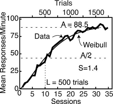
Group-learning curves have often been published. Fig. 1 is an example. In such a curve, the behavioral measures have been averaged across subjects; and often, across blocks of trials, or even whole sessions, as in Fig. 1. It is often assumed, either explicitly or implicitly, that the properties of the group curve are those of the individual curves. It has, however, long been recognized that averaging across subjects might give a misleading picture of what occurs in individual subjects (1–8). If the progress of conditioning in each individual subject is step-like, but the step occurs early in some subjects and later in others, averaging across subjects will suggest a gradual increase. Averaging across trials will also make rapid transitions appear to be more gradual.

Fig. 1.

Group-average (n = 20 pigeons) rate of key pecking (the conditioned response in the pigeon autoshaping paradigm) as a function of number of sessions (with 50 trials per session). Coordinate frame and jagged data line were traced from Gamzu and Williams (figure 2 in ref. 10, p. 227). We have superposed a Weibull function approximation (smooth curve), to show that this function, y = A {1 – 2^{^} – [(x/L)^{^}S]} can capture the kind of prolonged increase seen in these averages. A is the asymptote and L is the onset latency or location (the value of x at which y is half of its asymptotic value). Note the value (1.4) of the shape parameter S, which determines the shape and steepness of the function.

The potentially misleading nature of the group learning curve becomes serious when modelers try to make their model of acquisition process approximate the group curve, rather than the curve typical of the individual subject. For example, Kakade and Dayan (9) set as a criterion for a successful model of conditioning its ability to capture the prolonged increase in performance seen in Fig. 1 (which they also take from figure 2 in ref. 10, p. 227). We now show that in most subjects, in most paradigms, the transition from a low level of responding to an asymptotic level is abrupt.

Visualizing Acquisition

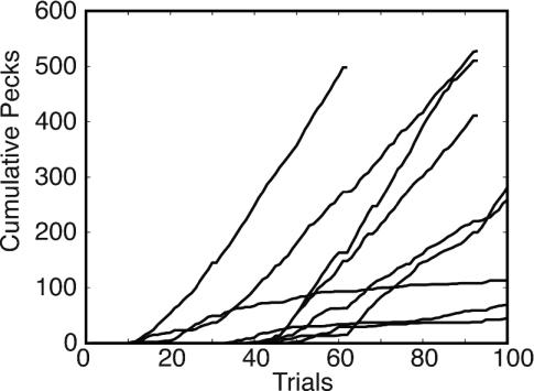
One way to visualize the course of acquisition is to plot the cumulative record of conditioned responses as a function of trials or reinforcements. The cumulative record is the running sum of the successive behavioral measurements. Changes in the slope of this record correspond to changes in the level of performance. Fig. 2 shows these plots for nine pigeons in one experimental group in an autoshaping paradigm, a commonly used appetitive Pavlovian paradigm. The illumination of a round key on the wall of the experimental chamber is the CS. The reinforcement is the brief presentation of a hopper filled with grain, which coincides with the end of the CS. The conditioned response is the pecking of the key. The pigeon pecks the key despite the fact that its pecking has no effect on food delivery. In this case, key illumination (the CS) lasted 6 sec and terminated with 4 sec of access to grain (the US). The average interval between key illuminations was 54 sec.

Fig. 2.

The cumulative number of pecks versus the number of trials for the nine birds in Condition CR_CS6_IT9.

Five things are apparent in these plots. First, the conditioned behavior seems to appear abruptly. The plots do not show the prolonged acceleration they would show if acquisition in the individual pigeon looked like the group average in Fig. 1. (This appearance, however, depends rather strongly on a choice of vertical scale. We describe methods for quantifying abruptness later in the text.) Second, asymptotic levels of performance (terminal slopes) differ greatly between subjects. Third, the latency, that is, the number of trials before the abrupt appearance of responding, also differs greatly between subjects. Fourth, there is little correlation between the two parameters; some records of shallow slope begin early and some begin late; conversely, some records with steep slope begin early and some late. Finally, it is not uncommon for the level of behavior to decrease later on, well below the level it had when it first appeared, as indicated by downward deflections in the slope of the cumulative record.

A second way to visualize the acquisition of conditioned responding is to plot the pecks on each trial (Fig. 3). This plot is the (discrete) derivative of the cumulative record plot. In some cases, it is readily intelligible (Fig. 3 Upper), whereas in others, the trial-to-trial variability in the number of pecks, makes it hard to see what is going on (Fig. 3 Lower). Other disadvantages of this visualization are that the parameters of acquisition (latency, abruptness, and asymptote) are not so readily visible, and, finally, one cannot make more than one plot per figure, to show differences and similarities between subjects.

Fig. 3.

Two examples of Pecks versus Trials plots. The dashed curve in each panel is the best-fitting Weibull function. (Upper) The subject did not respond at all for ≈40 trials; then, within the space of ≈10 trials, it transitioned to making between 5 and 15 pecks on each trial. These data are summarized fairly well by the best-fitting Weibull function. (Lower) The subject did not respond at all for the first 30 trials; then, it began to make between zero and three pecks per trial. This pattern of weak and highly intermittent responding persisted for 600 more trials. Although the plot is visually confusing, the Weibull function again captures the structure of the data. The asymptote is at 0.5 pecks per trial because the subject did not peck on substantially more than half the trials. The function rises with step-like abruptness, because after the first trial on which there was a peck (Trial 30), there was no further increase in the weak and intermittent pecking tendency. In fact, there was a modest decrease after Trial 200.

Quantifying Acquisition

In quantifying the appearance of conditioned behavior in individual subjects, we want to know at least three things: (i) how long it took for it to appear; (ii) how abruptly it attained its asymptotic level; and (iii) what the asymptotic level was. We now describe how to obtain these parameters from each kind of plot, beginning with the second kind.

Our approach to these questions is descriptive rather than model-driven. We use two different representations to test whether the conclusions one draws about acquisition depend on the choice of a representation.

We summarize the plots of pecks versus trials by fitting a continuous function to the data. The Weibull function is often used to summarize psychometric plots. When applied to the pecks-versus-trial data, the function is

Its parameters, A, L, and S, correspond to the aspects of acquisition just mentioned: asymptote (A), latency (L), and abruptness of onset (S).

Different values for the S parameter of the Weibull function cause it to assume widely different forms so it can approximate most monotonically increasing data sets. When S is close to 1, it approximates the inverse exponential. When S is >1.5, it is sigmoidal; asymmetrically so for values around 2, and symmetrically for values of 4 and higher. As S goes to infinity, it becomes a step function. Roughly speaking, the higher the value of S, the more abrupt the rise. However, it is important to bear in mind that this measure of abruptness is normalized to the L of behavioral onset, because S is the power to which the ratio Trials/L is raised. When the onset L is short, low values of S may be found in data that show a rapid initial rise in the level of performance (for example, see Fig. 7).

Fig. 7.

Determination of the dynamic interval, by using either the Weibull representation or the steps representation. This data set had the lowest value (0.49) for the S parameter of the Weibull function among the 105 data sets analyzed. Nonetheless, the initial rise is very rapid because the onset latency is so short (seven trials). The dynamic interval based on the Weibull representation is the number of trials between the first and ninth decile. The dynamic interval based on the Slopes representation is the number of trials between the first upward change point and the change point at which the postchange point slope is >80% of the asymptotic rate.

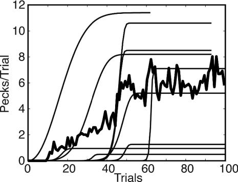
Summarizing the Pecks versus Trials plots with Weibull functions allows one to plot the results from all subjects on a single graph. Such a plot (Fig. 4) confirms the impression one has from the plot of the cumulative records: acquisition is generally abrupt, there are striking between subject differences in both onset latency and asymptotic level, and these differences do not covary.

Fig. 4.

Best-fitting Weibull functions for the Pecks versus Trials plots of the nine subjects whose data were first shown in Fig. 2 (smooth curves). The heavy jagged line is the group-average pecks per trial.

The Weibull function is monotonic; it cannot capture multistep changes in behavior, particularly when these postacquisition steps are both up and down. For that result, our second approach, based on the cumulative record is needed. We think that, generally speaking, the cumulative record is the best way to make the characteristics of the raw data immediately intelligible (cf. 11 and 12), because changes in behavior appear as changes in its slope. The points where such changes occur are change points. We have generalized a recursive algorithm (13) so that it may be applied to the finding of change points in any kind of cumulative record.

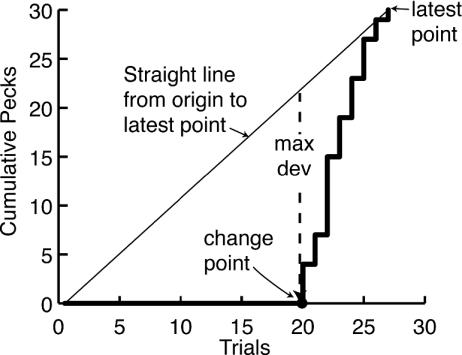
The algorithm has four stages: In the first stage, it identifies for each point in the cumulative record a putative change point in the record before that point. To find this earlier point, it in effect draws a straight line between the start of the record and the latest point and finds the earlier point that deviates maximally from this straight line (see Fig. 5). In the second stage, it computes for each putative change point, the strength of the evidence that it is a true change point. The strength of the evidence is the log of the odds against the null hypothesis of no change (the logit). In the third stage, it finds the first change point for which the evidence exceeds a user-specified decision criterion, and it truncates the data at that point. In the fourth stage, it begins over again, taking the change point as the origin and the first datum after the change point as the first observation.

Fig. 5.

In this illustration, the algorithm for finding change points is applied to the cumulative record as of Trial 27. (In practice, it is applied iteratively to each successive point in the cumulative record.) In this record, there were no pecks until Trial 20, where pecking began. The slanted dashed line is a straight line drawn between the origin and the cumulative record at end of Trial 27. The cumulative record deviates maximally from this straight line between Trials 19 and 20, so that is the putative change point. It divides the record up to Trial 27 into two portions: Trials 1–19 and Trials 20–27. If the change point is accepted as valid, then the algorithm begins over again, with the pecks on Trial 20 as the first datum.

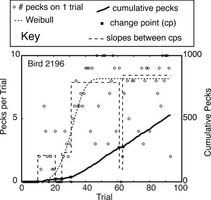
This procedure represents the behavior as a sequence of levels of performance. Each level is the slope of the cumulative record between two successive change points (Fig. 6). The number of successive levels in this representation depends on the decision criterion in the third stage of the parsing algorithm. The lower the decision criterion is, the more sensitive the algorithm is to possible changes in the level of performance; hence, the more change points it finds. For the representation in Fig. 6 (dashed steps), the decision criterion was set at logit = 2, which is rather sensitive. One may doubt that the two brief downward steps in the level of performance are to be taken seriously. It is likely that, at this level of sensitivity, the algorithm overfits the data, by using more segments than are necessary to capture the systematic structure of the data. One could use Bayesian and/or minimum-description-length techniques (14, 15) to limit the number of steps used to represent the complete record. However, these more complex methods are more appropriate when one is attempting to find a mathematical model of the process that generated the data. Here, we are only interested in a useable quantitative description. We routinely vary the sensitivity to see the effect that it has on the resulting representation and the summary statistics derived from it.

Fig. 6.

Different representations of the course of the acquisition of key pecking by a pigeon in a Pavlovian appetitive conditioning experiment. Data are either the number of pecks on each trial (left axis) or the cumulative number of pecks (right axis). The first representation is by means of a Weibull function fit to the pecks per trial (dotted curve). The second is by means of the slopes of the straight lines connecting successive change points in the cumulative record (dashed sequence of steps). These slopes are the average pecks per trial between two change points. The change points, as found by the change-point algorithm, are superposed on the cumulative record (▪).

With this approach to representing the data, the number of trials preceding the first upward change (the first significant increase in behavior) is the measure of the onset latency. The estimate of the asymptote is the mean response rate over the second half of the trials.¶ The abruptness of the transition is the number of trials between the first upward change point and the change point after which the postchange slope is ≥80% of the asymptotic rate. The measure depends on the decision criterion used in determining change points, so we repeat it by using criteria ranging from very sensitive to very insensitive.

The change-point-based measure of abruptness may be compared to an abruptness measure obtained by calculating the interval over which the best-fitting Weibull function rises from 10% to 90% of its asymptote.∥ Both approaches estimate the interval within which the rise in performance traverses 80% of its range. Fig. 7 illustrates the two measures of the dynamic interval.

Results

Autoshaped Key Pecking in the Pigeon. The choice of representation does not affect the conclusion that the appearance of autoshaped key pecking is abrupt. We subjected the data from 105 birds taught to key peck by continual reinforcement of transient key illuminations (that is, reinforcement on every illumination) in the laboratory of the late John Gibbon (Columbia University and New York State Psychiatric Institute). The data came from a variety of experiments, none of which was designed for the purpose of portraying the course of acquisition. The experiments differed widely in the duration of the CS, the duration of the intertrial interval, and some other parameters (e.g., whether there were one or two CSs and whether both or only one of them was reinforced). Depending on the analysis, between 22% and 56% of the birds went from a negligible level of responding to a nearly asymptotic level in a single trial. Between 45% and 57% made the transition in 10 trials or less. For 75% of the subjects, the dynamic interval was 34 trials or less, according to the change-point analysis with the most sensitive decision criterion, and 62 trials or less, according to both the Weibull analysis and the change-point analysis with the least sensitive criterion. Regardless of the analysis, ≈50% of the subjects made 10 or fewer responses within the dynamic interval.

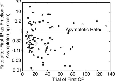
Another way to capture quantitatively the abruptness of the rise in conditioned behavior is to compute the rate of behavior after the first change point (that is, between the first and second change points) as a fraction of the asymptotic rate of behavior. We call this statistic the “first fraction.” Fig. 8 plots the first fractions as a function of the trial at the first change point. The median first fraction is 0.44, but the values range widely. To be noted, are the many cases in which the initial rate is higher than the asymptotic rate. Also to be noted is the lack of dependence on the latency: first fractions are not notably smaller in subjects with a long onset latency.

Fig. 8.

The rate of pecking between the first and second change points (determined by using t test and criterion = 2) as a fraction of the asymptotic rate of pecking, on a log scale, plotted as a function of the trial at the first change point.

The S parameter of the best-fitting Weibull function is a fourth way to index the relative abruptness of the rising phase: the higher the value of S, the more abrupt the transition, relative to the onset L, which, when the Weibull function is used, is the number of trials to a half-asymptotic level of performance. From the value of S, one can calculate what fraction of the period before and after the appearance of behavior is occupied by the transitional phase. For the median value of S, performance exceeds 10% of asymptote only when the number of trials has reached 82% of the onset latency. It attains 90% of the asymptotic level 0.15 log units later, when the trial count reaches 114% of the onset latency.

Correlations Between Parameters of Learning Curves. The correlation between the asymptote (A) and the onset latency (L) was weak (0.05) and insignificant, as was the correlation between the onset latency and the relative sharpness of the rise (–0.08). The correlation between the latency and the dynamic interval was positive (0.64). Thus, a late onset predicts a more gradual rise, when the rise is measured in absolute terms (number of trials over which rise occurs) but not when it is measured in relative terms (as a proportion of the onset latency or location, L). A late onset does not predict a lower asymptotic level of performance. Thus, the factors that determine how long it takes before conditioned behavior appears have little in common with the factors that determine how vigorous it is once it appears. This finding is important because the group-average learning curve confounds these two aspects of conditioned behavior: An early rise in the group average may indicate either that several subjects began to respond early or that a few subjects with a high postacquisition response rate happened to begin responding early.

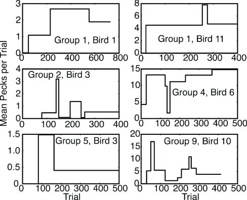
Bidirectional Changes in Performance Postacquisition. Representing the learning curve with a Weibull function presupposes that the increase in performance as a function of experience is monotonic. However, the algorithm that finds changes in the level of performance and represents performance as a sequence of levels reveals that this is often not the case. In the majority of the birds (56 of 105), there was at least one significant decrease in performance after the initial rise to “asymptote,” even when we used an extremely conservative decision criterion in the change-detecting algorithm, namely, logit = 6, which corresponds to odds of 1,000,000:1 against the hypothesis of no change (i.e., to P « 0.001). Fig. 9 shows examples chosen at random.

Fig. 9.

A random sample of the diverse but commonly seen ups and downs in the level of conditioned responding after its first appearance. The change points that generated these plots were detected by using the change-detecting algorithm, with a t test and a decision criterion (logit) of 6, which corresponds to a P value of <0.000001. Significant, substantial, and long-lasting decreases in performance are often seen. In other words, conditioned performance is asymptotically unstable.

As the diversity seen in examples in Fig. 9 makes clear, the pattern of postacquisition ups and downs in the level of performance varies greatly from subject to subject, and so resists summary. Some points, however, seem clear: First, postacquisition ups and downs in performance are large. Second, the level of performance seen hundreds of trials postacquisition may be a small fraction of the level seen soon after the first appearance of conditioned behavior. Third, the changeable character of postacquisition performance needs to be born in mind when one sees cases where there is a sequence of ascending steps. When both ascending and descending steps are common, then one expects to see occasional examples of an ascending sequence of several steps just from the chance arrangement (sequencing) of random steps of various size and sign. Finally, in this paradigm, the notion of running subjects until a stable asymptotic level of behavior is obtained is illusory, because up or down changes in the level of performance occur abruptly and unpredictably many hundreds of trials postacquisition.

Eye-Blink Conditioning in Rabbit and Rat. The eye-blink paradigm is a widely used aversive Pavlovian conditioning paradigm, particularly in neurobiologically oriented work. J. Kehoe (University of New South Wales, Sydney) kindly supplied data on 24 rabbits given delay eye-blink conditioning to a 650-ms tone (the CS), with one of three intervals; 200, 400, or 600 ms, between tone onset and the US (periorbital shock). There were 65 trials per 61-min session for the first 4 days and 80 trials per 75-min session for the remaining 3 days. The US was omitted on a random 8% of the trials. A conditioned response was scored when a blink followed the onset of the CS and preceded the US.

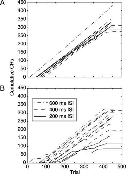
One subject never acquired a conditioned response. For 10 of the 23 subjects that did, the cumulative records show strikingly abrupt one-trial transition from no responding to a >80% probability of a conditioned blink (Fig. 10A). In the other subjects, either the transition or the subsequent responding is more variable (Fig. 10B), but the abrupt onset of nearly asymptotic responding predominates in the overall picture. When the records are analyzed with the change-point algorithm, using the binomial probability test with a decision criterion of 2 (equivalent to P < 0.01), the median dynamic interval is 1 trial and the median first fraction is 0.98.

Fig. 10.

Cumulative records of conditioned blinks from Kehoe's data. (A) Records of the most abrupt and steadiest rabbits. (B) The more variable records from Kehoe's data.

There is a significant negative correlation between onset latency (trials to first blink) and asymptotic responding, whether the asymptote is taken to be the blink probability over the second half of the trials (r =–0.73) or the maximum sustained blink probability (r = –0.59). Thus, a late onset predicts a lower asymptotic blink probability. The correlation between onset latency and the dynamic interval is insignificant (r = 0.11); a late onset does not predict a slow transition.

Similarly abrupt onsets of conditioned responding were seen in data supplied by D. Bangasser, D. Wexler, and T. Shors (Rutgers, The State University of New Jersey, New Brunswick) on the course of trace eye-blink conditioning in six rats. The CS was a 250-ms white noise. It was followed 500 ms after its offset by a mild periorbital electric shock. There were two sessions, with 200 trials each. The median dynamic interval was one trial and the median first fraction was 1.25.

There were large and prolonged fluctuations in postacquisition blink probability in both the rabbit and the rat data.

Conditioned Hopper Entry in the Rat. M. Bouton (University of Vermont, Burlington) kindly provided data from a hopper-entry autoshaping experiment conducted in his laboratory by M. Caniga, with eight rats as subjects. There were two 10-sec CSs, a 3,000-Hz tone, and a clicker, only one of which was reinforced. The positive, that is, reinforced CS was counterbalanced across subjects. Two food pellets were released into the feeding hopper at the conclusion of each positive CS; nothing happened at the conclusion of the negative (unreinforced) CS. The conditioned response was the anticipatory poking of the head into the feeding hopper. There were three presentations of the positive CS and three of the negative CS in each 90-min session, randomly intermixed. The interval between presentations varied about a mean of 15 min. The ratio between the intertrial interval and the signal interval (the trial duration) was much greater than in any of the pigeon autoshaping experiments. This ratio is known to lead to rapid acquisition (16), and it did so in this case. The mean acquisition latency in the Weibull analysis (the mean number of the trial at which performance attained half of its asymptotic value) was 5.8 (median 5.3). The mean and median of first change points were both 4.5, using a t test, with the decision logit set at 2.

The learning curves for rat autoshaping also rose abruptly. By using the change-point analysis, with the t test and a decision criterion (logit) of 2, the mean dynamic interval was 5.5 trials (median 6.5). (The asymptote estimates used in making this analysis were from the best-fitting Weibull functions.) The mean and median first fractions were both 0.61. The experiment stopped after 42 trials (14 sessions), so one cannot say whether one would see in this paradigm the postacquisition ups and downs seen in pigeon autoshaping and rabbit and rat eye-blink conditioning.

The Weibull A and the Weibull L (that is, trials to half-maximal responding) were weakly and insignificantly correlated (r = 0.26). The correlation between the trial at the first change point and the dynamic interval (interval between the first change point and the change point after which the slope exceeded 80% of the asymptotic slope) was –0.69. In words, the later the first appearance of conditioned behavior, the shorter the interval over which it rose.

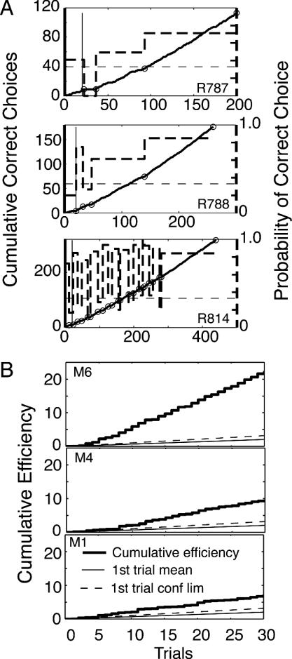
Plus Maze Learning in the Rat. D. M. Smith in the laboratory of S. Mizumori (University of Washington, Seattle) kindly provided data from 11 rat subjects in an experiment in which they learned to choose the baited arm in a four-armed maze in the shape of a plus. On each trial, the rat was placed facing the far end of a randomly chosen unbaited arm. In the first session, which consisted of 20 trials, the baited arm was chosen at random from one trial to the next. Thus, there was no possibility of nonchance performance. (There is a one-third probability of choosing the baited arm by chance.) After the first session, sessions consisted of 30 trials each. The baited arm changed half way through each session: for the first 15 trials of each session, the bait (two drops of chocolate milk) was at the end of the east arm; for the second 15, it was at the end of the west arm.

The measure of behavior in this paradigm is again binary (correct versus incorrect choice), so the change-detecting algorithm used the χ² test to assess the evidence that the frequency of correct choices after a putative change point was different from the frequency before.

Fig. 11A shows the cumulative correct choices for three of the 11 subjects. These are the solid lines plotted against the left axis of each panel. The small circles superposed on these lines are the change points found with a sensitive decision criterion (logit = 1.7, corresponding to a P value of 0.02). The heavy dashed lines plot the slopes between these change points against the right axis of each panel. These slopes are the probabilities of a correct choice. The end of the 20-trial pretraining period is indicated by a thin vertical line. The chance level of performance is indicated by a thin dashed horizontal line at 0.33 (right axis).

Fig. 11.

Spatial learning. (A) Three examples of cumulative correct choices in a plus maze (solid curves, plotted against the left axes) as a function of elapsed trials, with significant change points superposed (small circles). The slopes between the change points (heavy dashed lines) are plotted against the right axes (probability of correct choice). The chance level of performance (0.33) is indicated by the thin dashed lines. The thin vertical line at Trial 20 indicates the end of the pretraining period, during which the bait was randomly relocated from trial to trial. Data were from D. Smith and S. Mizumori. (B). Three examples of cumulative efficiencies for mice in a water-maze paradigm. The efficiency is the straight line distance from the point of placement to the platform divided by the distance swum. For reference, each plot also has lines with slopes equal to the group mean on the first trial and the group mean + 2 SE.

For most subjects, acquisition was abrupt and early. When we used the 1.7 decision criterion (P < 0.02), the median first fraction was 0.88 (0.90 when we used a still more sensitive decision criterion of 1.3, which corresponds to P < 0.05). The median dynamic interval was one trial. In 7 of 11 rats, the first positive increment in the probability of correct choice was >80% of the asymptotic increment. In the early sessions, some rats (notably, R814) did not adjust at first to the midsession reversal in the baited location, whereas others adjusted to this from the outset.

The majority of subjects began to choose correctly immediately after the end of pretraining: the first above-chance increment in correct choice probability was localized to within ± 5 trials of the end of pretraining in 6 of 11 rats (7 of 11 when we used logit = 1.3). This variability in the estimated change point reflects mostly the errors inherent in estimating exactly when the change occurred. Our procedure does not deliver a confidence limit for this estimate, but because the errors were as often negative as positive, that is, the change point was often located in the pretraining phase, where it could not in fact have fallen, we assume that all these changes in fact occurred at the start of the training phase, when the bait location first became predictable from trial to trial The first positive change point was within one trial of the first (east-west) reversal of bait location in one rat and within four trials of the beginning of the second training session in three rats.

In summary, what one sees in this appetitive spatial conditioning paradigm is one-trial learning. More often than not, the learning occurred on the first trial on which it could occur. In any case, what varied was not the gradualness with which correct choices emerged but rather the latency of the step-like appearance of an asymptotic level of correct choice. The data are consistent with the assumption that the subject notes the location on each trial and decides at some point that it is predictable from trial to trial.

Water-Maze Learning in the Mouse. In the water-maze paradigm, the subject is placed in a random location and orientation in a circular bath filled with opaque water, with a platform located somewhere just beneath the surface of the water. If it swims to the platform, it can stand on it. The platform must be discovered by random swimming on the first trial, but it remains in the same location on subsequent trials. With repeated trials, mice and rats learn to swim to it more directly. The paradigm is widely used in tests of the effects of genetic manipulations on spatial learning.

We applied our analytic procedures to data on the water maze learning of nine mice, kindly provided by R. Han and L. Matzel (Rutgers, The State University of New Jersey). On the first 30 trials of training, they videotaped the mice swimming until they reached and remained on the platform. From the tapes, they computed the efficiency of the mouse's swim, which is the straight-line distance between where it was placed and the platform divided by the distance the mouse swam in getting to and standing on the platform. Fig. 11B shows the cumulative efficiency records for three of the mice; the best, the median mouse, and the worst. For comparison, each record shows a line with a slope equal to the mean efficiency of all nine mice on the first trial (when they could not know where the platform was). It also shows a second (dashed) line with a slope equal to twice the SE of this mean. From this result, it can be seen that all mice achieved a greater efficiency than would be expected from the first-trial performance of the group. However, there were striking individual differences, and these differences were apparent from the outset. Some mice did much better than others.

These records were analyzed for change points by using the t test, with a decision criterion of 2.0 (P < 0.01). Most mice only had a single upward change point. There were three cases with two successive upward steps, but in two of them, the second upward step was followed by a downward step. In other words, there was no gradual improvement in the performance of any of these mice. Their performance went abruptly to asymptote. In short, these results are consistent with the previously ventured generalization: the learning of a spatial location generally requires but a single experience. Several trials may, however, be required to convince the subject that the location is predictable from trial to trial.

Discussion

The Nature of Learning. The change in conditioned behavior that occurs in the course of a typical conditioning experiment does not extend over many trials. Conditioned behavior commonly makes its appearance abruptly, going from its initially measured level to approximately its final level in the span of 1–10 trials.

The psychometric function for the detection of a light flash under optimal circumstances in the human observer undergoes 80% of its rise over an interval of ≈0.5 common log units of light intensity (17). The psychometric function for the detection of a tone embedded in noise undergoes 80% of its rise over of an interval of ≈0.9 common log units increase in sound intensity (18). By comparison, the median learning curve in pigeon autoshaping undergoes 80% of its rise in the span of a 0.15 log unit increase in training duration. Thus, the transition from the initial response level to vigorous responding in many conditioning experiments is more abrupt than the transition from undetectable to perfectly detectable in sensory threshold experiments.

The purely empirical conclusion that the typical learning curve undergoes most of its rise in the span of a few trials is not consistent with the totality of the following common theoretical assumptions: (i) underlying the appearance of simple learned behavior is the gradual strengthening of one or more associative connections; (ii) the relation between associative strength and number of reinforcements obeys, at least to a first approximation, first-order kinetics: it grows rapidly at first and then more slowly, approaching an asymptote exponentially; and (iii) measures of the strength of the learned response reflect this growth over an appreciable range of associative strengths. In other words, gradations in the behavioral measures reflect gradations in the underlying associative strengths. If all three of these assumptions were true, then individual acquisition curves would look like the group-average curve in Fig. 1, but they do not; they look like the curves in Fig. 4. Therefore, one or more of these assumptions is likely to be wrong. In this section, we consider alternatives to them.

One alternative is that learning is not associative, even in simple Pavlovian appetitive and aversive conditioning paradigms. From an information-processing perspective (16, 19–22), learning is the extraction from experience of information about the world, which is carried forward in memory to inform subsequent behavior. On this view, the brain computes from the information carried forward in memory the value of decision and control variables. A conditioned response appears when the value of the relevant decision variable exceeds a decision criterion (threshold). Once sufficient experienced has accrued so that the subject has decided to respond to the CS, the value of the decision variable is irrelevant to subsequent performance. Other variables, some experiencedependent, some not, determine the vigor of the postacquisition (postdecision) responding.

From an information-processing perspective on learning, the appearance of conditioned behavior is likely to be abrupt, for the same reason that psychometric functions in stimulus detection experiments are abrupt. Decision variables, unlike associative strengths, reflect the strength of the evidence that a behaviorally relevant state of the world actually obtains (for example, the strength of the evidence that the CS reliably predicts reinforcement). The strength of the evidence may be an accelerating function of the amount of experience. In this information-processing view, the abruptness of the onset of conditioned behavior is jointly determined by the steepness of this function as it crosses the decision threshold, the noise in the decision variable and the noise in the threshold. If the signal-to-noise ratio in the vicinity of the decision criterion is of the same order of magnitude as the derivative (slope) of the decision variable as it crosses the decision criterion, then conditioned responding will appear at full strength within the span of a few trials.

Within the associative framework, one can accommodate the step-like nature of the learning curve in individual subjects in at least two ways. One can assume that the underlying process of association formation is itself step-like. There is precedent for this in the older verbal learning literature (5, 23, 24), where it was shown that learning to recall a given word in a list of repeatedly presented words occurs in an all-or-nothing manner. This result led quite naturally to the assumption that the formation of an association was all or none.

However, the assumption that associative connection is all or nothing has no currency in the literature on animal learning and the neurobiology of learning. It requires, among other things, that one abandon the notion of a rate of learning, which is commonly understood to be the magnitude of the increment in associative strength on a reinforced trial normalized by the difference between the pretrial associative strength and the maximum possible strength.

Alternatively, one can continue to assume that simple conditioned behavior is mediated by the gradual, negatively accelerated increase in the strength of an underlying associative connection (or connections) but that performance factors prevent our observing this in the behavior itself. It is commonly and plausibly assumed that there is a behavioral threshold, below which an associative connection has no behavioral manifestation. Furthermore, the behavioral manifestation of a given increment in associative value may translate into different behavioral changes depending on where one is on a performance function (25, 26). It is also plausible that there is a behavioral saturation level for associative strength, a level above which further increases in associative strength produce no further increase in the vigor, rate, or probability of a conditioned response. The question then is whether the behavioral threshold and the saturation level are sufficiently far apart for any appreciable range of associative strengths to be manifest in a range of behavioral strengths. The narrow dynamic intervals that predominate in the individual learning curves analyzed here imply that the behavioral threshold and the saturation level are so close together that a negligible portion of the function relating associative strength to number of reinforcements is visible.

Under these narrow-window assumptions about the performance function, the common associative model becomes similar in important respects to the information-processing model. There is in both an underlying quantity that grows with experience until it crosses a threshold, above which its value is behaviorally irrelevant. The conclusion that the performance function (the narrow distance between threshold and saturation levels) makes only a negligible portion of the associative growth function behaviorally visible implies that neither the form nor the parameters of the underlying growth function may be estimated even approximately directly from the behavioral learning curve. Because, by assumption, the asymptote, if any, of the underlying function lies above the behavioral saturation level, the asymptotic strength of the measured behavior does not depend on the asymptote of the growth function. In other words, asymptotic behavioral strengths do not provide even an ordering of the underlying associative strengths. The latency to behavioral onset is similarly uninformative. It may be increased or decreased either by raising or lowering the narrow behavioral window, by decreasing or increasing the rate of learning (the steepness with which the underlying growth function rises), or by increasing or decreasing asymptotic associative strength. The implications of this conclusion for the interpretation of results from experiments that look for genetic or pharmacological effects on the rate of learning are unpalatable. From the learning curve alone, it would not seem possible to distinguish effects on performance factors from effects on association formation.

None of these conclusions will surprise some students of animal learning, who have generally ignored the effects of training variables on the learning curve in favor of designs that compared the effects of various treatments on the asymptotic level of behavior. However, these designs rarely test whether behavior has in fact attained an asymptote, and they often rely on the assumption that asymptotic strength and rate of acquisition covary and that the ordering of asymptotic behavioral strengths indicates the ordering of underlying associative strengths. Our analysis shows that none of these assumptions is empirically justified.

The Elusive Asymptote. We have referred repeatedly to the behavioral asymptote, and we often made use of an estimate of it in our analyses, while at the same time, presenting evidence that throws doubt on the existence of an asymptote in the strict sense. Strictly speaking, a performance asymptote exists only if there is a stable value to which performance approaches arbitrarily closely as one extends training for arbitrarily many trials. The performance of many subjects in many different paradigms appears never to attain an asymptote in that sense. Rather, it appears to fluctuate irregularly. The postacquisition instability of conditioned behavior would be consistent with the presence of substantial 1/f noise in these repeated behavioral measurements. This kind of variability, is ubiquitous in repeated behavioral measurements (27). The f in 1/f noise refers to the frequency parameter in a Fourier analysis of the sequence of behavioral measures. The inverse of the frequency is the period of an oscillation, the number of trials, or the temporal interval required for a complete oscillation. In 1/f noise, the amplitude of the oscillation, how far it diverges from its mean value, is proportional to the period of fluctuation. Thus, long-lasting variations in performance are large; indeed, the longer lasting they are, the larger they are. In data, with 1/f noise, there is no asymptote in the strict sense. Moreover, estimating the mean about which the data fluctuate is complicated by the fact that the longer the period of the fluctuations one observes, the larger are their amplitudes. Thus, extending the period over which the mean is estimated may not improve the estimate. There may be no alternative to the kind of rough-and-ready estimate we have used.

Implications for Good Practice. The group-average learning curve confounds three independent parameters of individual learning curves, onset latency, dynamic interval, and asymptote. From the group-average curve, it is not possible to determine which of these parameters differs between the groups, or even if there are consistent differences.

The methods we have elaborated in these analyses show how to improve the common practice. Whatever is measured on each trial, it possible to produce from it a cumulative record, by computing trial by trial the cumulative (running) sum. When plotted, this cumulative record allows one to see at a glance the onset latency, the abruptness or gradualness of the approach to asymptote, and the asymptotic level (terminal slope), if there is one. A dozen or more cumulative records can be plotted on a single graph (Figs. 2 and 10). Thus, it is possible to lay the plots for the subjects in the control and experimental groups side by side or one above the other, giving a visually comprehensible, information-rich presentation of the data from every subject in every group. The algorithm for computing change points and the slopes between them translates what the viewer sees into a representation of the record, from which summary statistics are easily computed. The algorithm is included in the supporting information, which is published on the PNAS web site.

The obvious summary statistics are the onset latency (the number of trials to the first change point), the dynamic interval and the first fraction (measures of the abruptness of the behavioral transition), some measure of the notional asymptote, and possibly, also, a measure of the postacquisition stability of the behavior. An example of the latter would be the maximum difference between postacquisition slopes (rates), divided by the notional asymptote. This measure gives an indication of the amplitude of prolonged postacquisition fluctuations in behavior.

Conclusion

The acquisition of conditioned behavior is probably not always abrupt. However, the range of data analyzed here establish a presumption of abruptness. In most cases, the learning curve for individual subjects may be assumed to rise from the level seen in the naive subject to a level characteristic of a well trained subject in <10 trials (indeed, often in a single trial). The postacquisition level of responding often shows large, prolonged fluctuations. Additionally, there is no consistent correlation between the latency to the onset of conditioned behavior and its subsequent vigor.

Given the abruptness with which conditioned behavior appears and the lack of consistent correlation between latency, abruptness and asymptote in the individual curves, the group-average learning curve cannot give a meaningful measure of rate of learning. The best measure of would appear to be the latencies to the onset of responding.

References

- 1.Lashley, K. S. (1942) J. Gen. Psychol. 26, 241–265. [Google Scholar]
- 2.Krechevsky, I. (1932) Psychol. Rev. 39, 516–532. [Google Scholar]
- 3.Estes, W. K. (1956) Psychol. Bull. 53, 134–140. [DOI] [PubMed] [Google Scholar]
- 4.Estes, W. K. (2002) Psychon. Bull. Rev. 9, 3–25. [DOI] [PubMed] [Google Scholar]
- 5.Restle, F. (1965) Psychol. Bull. 64, 313–325. [DOI] [PubMed] [Google Scholar]
- 6.Brown, S. & Heathcote, A. J. (2003) Behav. Res. Methods Instrum. Comput. 35, 11–21. [DOI] [PubMed] [Google Scholar]
- 7.Hanson, S. J. & Killeen, P. R. (1981) J. Exp. Psychol. Anim. Behav. Processes 7, 129–139. [Google Scholar]
- 8.Cousineau, D., Hélie, S. & Lefebvre, C. (2003) Behav. Res. Methods Instrum. Comput. 35, 493–503. [DOI] [PubMed] [Google Scholar]
- 9.Kakade, S. & Dayan, P. (2002) Psychol. Rev. 109, 533–544. [DOI] [PubMed] [Google Scholar]
- 10.Gamzu, E. & Williams, D. R. (1973) J. Exp. Anal. Behav. 19, 225–232. [DOI] [PMC free article] [PubMed] [Google Scholar]
- 11.Skinner, B. F. (1976) J. Exp. Anal. Behav. 25, 218–221. [DOI] [PMC free article] [PubMed] [Google Scholar]
- 12.Killeen, P. R. (1985) The Behavior Analyst 8, 177–183. [DOI] [PMC free article] [PubMed] [Google Scholar]
- 13.Gallistel, C. R., Mark, T. A., King, A. P. & Latham, P. E. (2001) J. Exp. Psychol. Anim. Behav. Processes 27, 354–372. [DOI] [PubMed] [Google Scholar]
- 14.Pitt, M. A., Myung, I. J. & Zhang, S. (2002) Psychol. Rev. 109, 472–491. [DOI] [PubMed] [Google Scholar]
- 15.Myung, I. J. & Pitt, M. A. (1997) Psychon. Bull. Rev. 4, 79–95. [Google Scholar]
- 16.Gallistel, C. R. & Gibbon, J. (2000) Psychol. Rev. 107, 289–344. [DOI] [PubMed] [Google Scholar]
- 17.Hecht, S., Shlaer, S. & Pirenne, M. H. (1942) J. Gen. Physiol. 25, 819–840. [DOI] [PMC free article] [PubMed] [Google Scholar]
- 18.Green, D. M. (1960) J. Acoust. Soc. Am. 32, 1189–1203. [Google Scholar]
- 19.Gallistel, C. R. (1990) The Organization of Learning (Bradford Books/MIT Press, Cambridge, MA).
- 20.Gallistel, C. R. (1999) in The Cognitive Neurosciences, ed. Gazzaniga, M. S. (MIT Press, Cambridge, MA), 2nd Ed., pp. 1179–1191.
- 21.Gallistel, C. R. & Gibbon, J. (2002) The Symbolic Foundations of Conditioned Behavior (Lawrence Erlbaum Associates, Mahwah, NJ).
- 22.Gallistel, C. R. (2003) Behav. Proc. 62, 89–101. [DOI] [PubMed] [Google Scholar]
- 23.Estes, W. K. (1960) Psychol. Rev. 67, 207–223. [DOI] [PubMed] [Google Scholar]
- 24.Rock, I. & Steinfeld, G. (1963) Science 140, 822–824. [DOI] [PubMed] [Google Scholar]
- 25.Rescorla, R. A. (2002) J. Exp. Psychol. Anim. Behav. Processes 28, 406–415. [PubMed] [Google Scholar]
- 26.Rescorla, R. A. (2000) J. Exp. Psychol. Anim. Behav. Processes 26, 428–438. [DOI] [PubMed] [Google Scholar]
- 27.Gilden, D. L., Thornton, T. & Mallon, M. W. (1995) Science 267, 1837–1839. [DOI] [PubMed] [Google Scholar]
Associated Data
This section collects any data citations, data availability statements, or supplementary materials included in this article.