

Abstract
Motivation: The vast amount of already available and currently generated read mapping data requires comprehensive visualization, and should benefit from bioinformatics tools offering a wide spectrum of analysis functionality from just one source. Appropriate handling of multiple mapped reads during mapping analyses remains an issue that demands improvement.
Results: The capabilities of the read mapping analysis and visualization tool ReadXplorer were vastly enhanced. Here, we present an even finer granulated read mapping classification, improving the level of detail for analyses and visualizations. The spectrum of automatic analysis functions has been broadened to include genome rearrangement detection as well as correlation analysis between two mapping data sets. Existing functions were refined and enhanced, namely the computation of differentially expressed genes, the read count and normalization analysis and the transcription start site detection. Additionally, ReadXplorer 2 features a highly improved support for large eukaryotic data sets and a command line version, enabling its integration into workflows. Finally, the new version is now able to display any kind of tabular results from other bioinformatics tools.
Availability and Implementation: http://www.readxplorer.org
Contact: readxplorer@computational.bio.uni-giessen.de
Supplementary information: Supplementary data are available at Bioinformatics online.
1 Introduction
During the last years next-generation sequencing (NGS) technologies (Bentley et al., 2008; Margulies et al., 2005) vastly changed the field of DNA and RNA sequencing by drastically reducing the costs while increasing the sequencing yield per run at the same time (Reuter et al., 2015). Nowadays NGS has a broader scope as ever and is currently entering the field of clinical microbiology for infectious disease diagnostics and epidemiology (Buchan and Ledeboer, 2014; Goldberg et al., 2015).
Whole genome sequencing and transcriptome sequencing (RNA-Seq) data sets are huge and comprise millions of reads, requiring proper and scalable data handling. A typical analysis workflow requires mapping of the reads to a reference genome followed by the respective analyses. This requires easily applicable automatic analyses and comprehensive visualization for read mapping data as implemented in the flexible ReadXplorer software (Hilker et al., 2014). The software is based on a quality classification of the read mappings and offers single nucleotide polymorphism and deletion–insertion polymorphism detection, genomic feature and general coverage analysis, RNA secondary structure prediction, differential gene expression analysis, transcription start site (TSS) detection, operon detection and RPKM value and read count calculations. Although not optimal, it is still common practice to exclude reads mapping to more than a single position from downstream analyses (Li et al., 2015) and many read mapping analysis tools do not address multiple mapped reads (e.g. TSSPredator (Dugar et al., 2013), TSSer (Jorjani and Zavolan, 2014) and TSSAR (Amman et al., 2014) for TSS detection or VarScan 2 [(Koboldt et al., 2012) for single nucleotide polymorphism (SNP) detection]. For the latter tools, we assume that they incorporate all reads present in the data set provided by the user. A notable exception is the RNA-Seq analysis tool Rockhopper (McClure et al., 2013). It uses all optimal alignments of a read, but it remains unclear how multiple mapped reads are taken into account when measuring the read count for a gene.
In contrast to common practice, various publications (Robert and Watson, 2015; Treangen and Salzberg, 2012) have shown the importance of properly handling multiple mapped reads instead of discarding them. Generally, relying on a single randomly chosen mapping position for a read leads to a possibly erroneous choice about read placement (Treangen and Salzberg, 2012), while in RNA-Seq experiments the exclusion of multiple mapped reads leads to underestimation of the data (Robert and Watson, 2015).
To accommodate these issues, the first version of ReadXplorer already featured a read mapping classification unique among read mapping visualization tools. For the current work, we focused on a further refinement of this read classification. Hereby, an even more detailed view on the mapping data is enabled and allows for easy configuration of the mapping classes included in all downstream analyses.
Besides the classification, the analysis capabilities of the software have been largely enhanced to offer both more detailed [differential gene expression, read count and normalization analysis and TSS detection] and new automatic analysis functions (genome rearrangement detection and correlation analysis). Further, we introduce technical improvements enabling integration of ReadXplorer 2 into larger pipelines or workflow systems such as our Galaxy server, improving speed, broaden the support of large eukaryotic data sets and simplifying the connection between GNU R (R Core Team, 2014) and Java.
2 Enhanced analysis capabilities
In the following, we present the enhanced read mapping classification, newly implemented analysis functions and substantial enhancements of existing analysis functions.
2.1 Extended read classification
For a more detailed distinction of the reads in comparison to the first ReadXplorer version, two additional read mapping classes have been added to the three existing ones (Perfect Match—a mapping without mismatches, Best Match—a mapping with less deviations than all other mappings of the read, and Common Match—a mapping of a multiple mapped read with better mappings with less deviations elsewhere) (see Table 1):
The Single Perfect Match class contains all reads with exactly one (single) perfect match.
The Single Best Match class contains all mappings that cannot be allocated to another position in the reference with the same number or fewer mismatches than at the current position - they exactly have one (single) best match.
Table 1.
Read mapping classification in ReadXplorer 2
| Read Mapping Classification | Properties |
|---|---|
| Single Perfect Match | Read has only one mapping without mismatches, may have additional Common Match mappings |
| Single Best Match | Read has one mapping with less deviations than all other mappings, may have additional Common Match mappings |
| Perfect Match | Read has multiple mappings without mismatches |
| Best Match | Read has multiple mappings with the same number of deviations from the reference |
| Common Match | Read has better mappings with less deviations to the reference |
The Perfect and Best Match mapping classes contain multiple mapped reads with equally good mapping positions, e.g. two perfect mappings without mismatches at different genomic positions. In contrast, the Single Perfect Match and Single Best Match class contain both uniquely mapped reads and the distinctive best mapping of multiple mapped reads. This extended classification enables quick discrimination of reads with only one distinctive best mapping from mappings with multiple equally scoring mappings, while not requiring the read to be uniquely mapped. Reads from both Single Match classes can have more mappings with lower quality, falling in the Common Match class. Thus, this classification is not as strict as only considering uniquely mapped reads with exactly one valid mapping to the reference. The extended read classification is not only used for visualization (Fig. 1) but also for read selection during the wizard based setup of all analysis tools offered by ReadXplorer 2. Hereby, additional use cases are enabled for the automatic analysis of read mapping data. As one example, the ‘Coverage Analysis’ can now be used to identify almost identical repetitive regions. By only selecting the Perfect, Best and Common Match mapping classes, only genomic intervals covered by multiple mapped reads—representing repetitive regions in the genome—are returned by the analysis. Such a region is depicted in Figure 1 by the light yellow, red and light green areas.
Fig. 1.
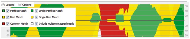
The five read mapping classifications in the coverage plot. Read counts per base of input sequence are shown separated by strand and colored by mapping classification. Reads aligning at the borders of the figure have a distinctive best mapping (Single Perfect and Single Best Match classes in rich green and yellow), while the light green (Perfect Match), light yellow (Best Match) and red (Common Match) mappings display a repetitive region
2.2 Read count normalization
The first ReadXplorer version featured an RPKM (total exon reads per million mapped read per kilobase of exon model) (Mortazavi et al., 2008) based read count analysis. This analysis has been enhanced by two additions: the model for assigning reads to a genomic feature was improved to allow for a more accurate way of read assignment to a feature and the TPM (Transcripts per million) (Li et al., 2010) normalization method was added to the analysis.
RPKM is meant to reflect relative molar concentrations of transcripts by normalizing for transcript length and library size. This type of normalization is necessary for reasonable comparisons of transcript abundances both within one and among multiple samples. TPM was proposed as an improvement to RPKM, because TPM has the advantage of being invariant between samples and species (Li et al., 2010) while RPKM values may change when the mean expressed transcript length changes due to different sets of active genes in two samples.
TPM is defined according to (Li et al., 2010) as
where c is the number of mappable reads for genomic feature i and j is an integer ranging from 1 to the number of genomic features of the same type (e.g. genes).
To take into account that reads of a given length cannot start at each position in a transcript, the effective length of transcripts can optionally be used for the normalization instead of the whole transcript length l. The effective length of transcript i was first defined by (Trapnell et al., 2010) as
where x is one of the observed read length values in transcript i of length li, and λF is the fraction of reads for i with length x.
The model for assigning reads to a transcript needs to be as precise as possible, because the normalization outcome is determined by the chosen transcript boundaries and the inclusion model for the reads. Our analysis offers to either use the given boundaries of genomic features or define a fixed offset for start and stop positions, separately. Using an offset can be useful when most of the 5′ and 3′UTRs are not taken into account by the genomic features of the reference. Additionally, automatically annotated gene start and stop positions might be incorrect, leading to data loss.
The implemented read assignment model for read mappings overlapping multiple genomic features (e.g. genes or coding sequence (CDS)) is similar to the union model of HTSeq-count (Anders et al., 2014) with one difference: we include read mappings of the two cases marked as ambiguous by HTSeq-count’s union model instead of discarding them (Supplementary Fig. S1). In the first case, reads fully contained in the first feature and overlapping the start of a second feature are associated to the first feature. In the second case, reads fully contained in two overlapping feature are counted proportionally for each of the overlapped features.
In addition to the general export functionality, the TPM or RPKM-value distribution of the analyzed data set can be visualized in a log-scaled histogram (see Fig. 2). All bin borders are dynamically calculated according to the percentage they contribute to the result.
Fig. 2.
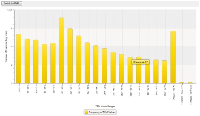
The histogram comfortably visualizes the frequency of TPM values observed within the data set at log scale. The actual number of features belonging to one bar is shown in the tooltip. It can be switched to show RPKM values
2.3 TSS analysis
The TSS detection has been substantially enhanced towards a more detailed analysis of TSS properties. In some cases the coverage increases in steps at a TSS. To consider this case, an option was implemented to associate all predicted TSSs within a small user-defined bp window to the statistically most significant TSS. Hereby, neither several predicted TSS appear for one gene, nor is any of them lost.
To identify at a glance if evidence for alternative TSSs exist, all identified TSSs within a user defined window are classified. The statistically most significant position is designated as ‘primary’ TSS, while all other TSSs on the same strand are marked as ‘secondary’. In many microbial organisms the majority of transcripts contains a leader, but transcripts can also be leaderless (Pfeifer-Sancar et al., 2013). To distinguish both cases easily, leaderless transcripts are flagged in the result and can thus be retrieved instantly. The maximum distance of a TSS to the actual translation start site can be adjusted in the wizard. To offer a deeper insight into novel transcripts identified by the analysis, the TSS detection further computes the next start codon on the respective strand, the leader length and the next in-frame stop codon. The novel transcript length is deduced from the assigned start and stop codons. Another new feature is the option to configure the length of exported upstream and downstream regions for promoter analysis.
2.4 Differential gene expression with DESeq2
To offer easy access to one of the most recent analysis tools for differential gene expression analysis, we added DESeq2 (Love et al., 2014) to the set of integrated tools. With baySeq (Hardcastle and Kelly, 2010) and the original DESeq (Anders and Huber, 2010) already integrated, ReadXplorer 2 offers three widely used analysis tools for identifying differentially expressed genes. The settings for the analysis can be easily specified by a step-by-step wizard in the same fashion as for the already integrated tools (Supplementary Fig. S2–S6).
2.5 Genome rearrangement detection
Genome rearrangements or structural variations (SVs) are associated to many diseases including cancer (Iafrate et al., 2004). In addition, genome rearrangement detection is useful for the phylogenetic analysis of eukaryotic and prokaryotic organisms.
In general, the tools for SV detection are command-line based. Integrating an established SV detection tool into ReadXplorer 2 makes genome rearrangement detection accessible for researchers unfamiliar with command-line tools and enables immediate visual inspection of read pair configurations in genomic regions with predicted SVs (see Fig. 3).
Fig. 3.

Visualization of genome rearrangement events using GASV (Sindi et al., 2009). ReadXplorer 2 offers an effortless exploration of the data underlying the genome rearrangements detected by GASV (table at the bottom). The region of the deletion selected in the table is centered simultaneously in the reference, track and read pair viewer. In the example, the hypothetical protein PA0343 is deleted in P. aeruginosa strain B420 from the study by Hilker et al. (2015). No reads map to the corresponding region of P. aeruginosa PAO1 and many read pairs are observed in B420 with an enlarged distance of about 1200 bp instead of the expected 300 bp
We chose Geometric Analysis of Structural Variants (GASV) 2.0 (Sindi et al., 2009, http://compbio.cs.brown.edu/projects/gasv/) for integration. Its development focused on the human genome, but it has also been tested successfully on other genomes like yeast (Zeitouni et al., 2010). GASV supports a broad range of rearrangements: insertions, deletions, inversions, translocations and can handle more divergent rearrangement events, i.e. resulting from multiple rearrangements at the same locus.
To guarantee flexibility for the user, the GASV wizard in ReadXplorer 2 offers all options available for the command line version of GASV.
Note that only Single Perfect Match and Single Best Match mappings are allowed for the GASV analysis. Testing different mapping classifications with different example data sets showed that it is inevitable to use only these two classes to produce reasonable results. Otherwise, repeat regions lead to many false positive rearrangement predictions obscuring the correct predictions.
2.6 Correlation analysis
A correlation coefficient can be used to identify regions of two tracks mapped to the same reference showing very similar or completely different coverage to identify similarities and differences in the data sets automatically. Two exemplary applications are: The comparison of two RNA-Seq data sets (e.g. a whole transcriptome and a 5′ enriched one) to identify all TSS regions correlating in both tracks and retrieval of all genomic regions with correlating expression patterns. To compare two tracks, we divide the genome into intervals of user defined length and perform statistical correlation analysis of the coverage value pairs for each position within each interval. The options are configured on a single wizard page, where the user can choose the correlation method and additional parameters. The two implemented methods to calculate the correlation coefficient are (i) the Bravais-Pearson (Pearson, 1895) product-moment and (ii) the Spearman’s rank (Spearman, 1904) correlation coefficient.
Spearman’s rank correlation coefficient has the advantage that no assumptions on the underlying probability distribution have to be made and no linear relationship is required between the random variables.
2.7 Visualization of split read mappings
For a correct visualization of eukaryotic RNA-Seq reads spanning an exon-intron boundary, the user interface was enhanced to display split read mappings in the Track Viewer, the Alignment Viewer and the Histogram Viewer. Analysis functions also take the mapped blocks of split read mappings into account.
2.8 Other analysis enhancements
Minor, but notable new features include: (i) Each analysis now offers the option to select the strand on which the reads are mapped in relation to genomic features (same, opposite or combine reads of both strands). (ii) The read classes of the reads used for an analysis can be selected and a minimum mapping quality threshold (Phred scale) can be set. (iii) All analysis results that are displayed in a tabular form can be exported as a comma separated values (CSV) file in addition to the Microsoft Excel file (XLS) export. (iv) The SNP detection was enhanced by base quality filter options (minimum average and minimum PHRED scaled base quality) and a minimum average mapping quality option. (v) The coverage analysis offers a button to export the underlying sequences of the intervals identified by the analysis to use them for downstream analyses (e.g. motif search, BLAST). (vi) The feature coverage analysis additionally lists the mean interval coverage. (vii) For reproducibility, each exported analysis table contains the ReadXplorer version number it was created with.
3 Technical improvements
ReadXplorer 2 is now based on Java 1.8 and Netbeans Platform 8. For an easy installation we offer stand-alone installers with an integrated Java Runtime Environment for Windows, Linux and Mac OS X.
3.1 Command line interface
In order to cope with data sets consisting of many tracks and to enable the integration of ReadXplorer 2 into automatic analysis pipelines, the software now provides a command line interface (CLI).
Via this new interface it is possible to concurrently import reference and mapping files, perform analyses and export results by providing corresponding parameters without the need for user interaction. Thus, executing a whole workflow is less time consuming than before. For the sake of usability all import and analyses preferences can be set in a separate configuration file which can be reused for future analyses.
This new feature allows command line users an easy and flexible integration of ReadXplorer 2 in any command line pipeline or automatic analysis scripts.
3.2 Rserve integration
For the differential gene expression analysis ReadXplorer 2 primarily relies on established tools only available for GNU R (R Core Team, 2014). In order to use these tools a Java to GNU R interface is needed. In ReadXplorer 2 we changed this interface to Rserve (Urbanek, 2003), offering an easier setup and a more stable execution of the analysis tasks. On Windows machines an automatic setup is offered, for Linux and Mac OS X the connection to an Rserve instance can easily be configured via the options menu.
3.3 Other implementation enhancements
ReadXplorer 2 can import tabular results (CSV, XLS, variant call format (VCF)) either created by itself or any other tool. This enables comparisons of ReadXplorer 2 generated results with the results created by other established tools and offers flexible visualization of analysis results from command-line tools.
A link was added for cross-linking genomic features with an EC-number to a user configurable enzyme database (default: ExPASy, http://www.expasy.org/).
The graphical user interface now offers a detailed viewer for combined tracks. Additionally, the alignment view of the detailed viewer is now zoomable and the bases are colored based on quality. The track viewer supports additional feature types for displaying (ncRNA, 5′, 3′UTR, RBS, −35_signal, −10_signal) and offers a new option to display all reads from both strands on the forward or reverse strand only. This is especially useful for visualizing data sets originating from non-strand-specific RNA-Seq experiments.
The complete mapping statistics of all tracks can now be exported from the database.
3.4 Web service
To ease the use of ReadXplorer 2, we added it to the toolbox of our Galaxy server at https://www.computational.bio.uni-giessen.de/galaxy/. The server is available for registered users only, but registration is free of charge. Here, we use the CLI to automatically create a ReadXplorer database for the user data and allow downloading the full data package after project calculation.
4 Results
We used ReadXplorer 2 for the evaluation of an Arabidopsis thaliana RNA-Seq test data set that was generated for this purpose. Several of the aspects described above were addressed, namely extended read classification, improved handling of eukaryotic data and the DESeq2 integration. The experiment focused on differential gene expression analysis between the A. thaliana Col-0 wild-type and a myb11-12-111 triple-mutant line (Supplementary Materials); array-based data for this biological material are available (Stracke et al., 2007). Three biological replicates, each of them consisting of two technical replicates, were created from wild-type and mutant each. The 12 samples produced ∼183 million usable reads that were mapped to the TAIR 10 A. thaliana Col-0 reference. Besides visual inspection, we started the analysis with a “read count and normalization calculation”, to check the integrity of the biological and technical replicates. This was achieved by plotting their TPM values against each other to check for correlation (Supplementary Fig. S7). For all except one technical replicate, the resulting expression values corresponded to each other (were located close to the 45° diagonal). Thus, the problematic technical replicate was excluded from further analysis. Further investigation showed that in the problematic sample rRNA removal was incomplete. This experimental complication occurs at low frequency with the RNA-Seq kits from Illumina.
To identify differentially expressed genes between the wild type and the mutant and simultaneously monitor the effect of employing the extended read mapping classification, we applied DESeq2 via ReadXplorer 2 twice with different included read mapping classes. Once, we only used the uniquely mapped reads and in the second case, we used the Single Perfect and Single Best Match mapping classes—also including reads with a distinctive best mapping. The latter selection enabled us to include on average 1 400 000 more reads per data set in the analysis (Supplemental Table S1), leading to more accurate gene expression values and minimizing underestimation of expression levels. This effect can be observed even in the most differentially expressed genes (Fig. 4). Two examples are the genes AT5G46900 and AT4G12510. Their mean expression is increased from 299 to 379 reads in the first case and from 135 to 189 reads in the second case. These and other examples (Supplementary Table S2) convincingly show that the level of differential gene expression is underestimated if only uniquely mapped reads are used. In total, the expression of 13 850 of all 28 775 annotated genes is underestimated. Of these, 1896 genes can be assigned > 100 and 153 genes > 1000 additional mappings when applying the extended read classification. The comparison of the DESeq2 results between only incorporating uniquely mapped reads and using the Single Perfect and Single Best Match mapping classes is shown in Supplementary Table S3.
Fig. 4.

The difference of the read coverage between only uniquely mapped reads (middle row) and using the ‘Single Perfect Match’ and ‘Single Best Match’ mapping classes is shown for the genes AT5G46900 and AT4G12510 (upper row). In total numbers 144 and 78 more reads can be included in the analysis respectively when using the extended read mapping classification (Color version of this figure is available at Bioinformatics online.)
Additionally, we show in Supplementary Table S4 that ReadXplorer 2 offers several unique features and combines many useful features that are not present in this composition in one of the other commonly used read mapping visualization tools like Savant (Fiume et al., 2012), Integrated Genome Browser (IGB) (Nicol et al., 2009), Artemis (Carver et al., 2012), Integrative Genomics Viewer (IGV) (Robinson et al., 2011) and GenomeView (Abeel et al., 2012).
Finally, we assessed the performance of analysis functions offered by ReadXplorer 2. We benchmarked the performance on small (∼6 mb), medium (∼120 mb) and large (∼3 gb) reference genomes (Supplementary Table S5). This assessment also includes a comparative runtime benchmark between ReadXplorer 1 and ReadXplorer 2 (Supplementary Table S6). The results show that on the same hardware the new version of our software significantly outperforms the older release when the same tasks are executed.
5 Discussion
The comprehensive read mapping data visualization and automatic analysis tool ReadXplorer 2 features substantially enhanced capabilities from one source. The major improvement presented here is the extended read mapping classification which leads to more specific analysis results as shown in the results section. Further, the extended classification enables meaningful integration of multiple mapped reads and creates awareness for the different types of multiple mapped reads, e.g. to identify repetitive regions (Fig. 1). Moreover, two newly implemented analysis functions and substantial improvement of existing analyses widen the spectrum covered by ReadXplorer 2 and enable the user to screen for genome rearrangements and correlation between two data sets without the need to install additional software. The read count normalization can now be compared between different samples as the added TPM normalization is invariant between samples. With DESeq2 another widely used differential gene expression analysis package is available from within the software. The enhanced TSS detection allows deeper insights into the TSS landscape by analyzing additional properties of the TSS and presenting them to the user. The application range of ReadXplorer 2 is further broadened by improving the handling of eukaryotic data.
Using our A. thaliana RNA-Seq data set, we were able to successfully evaluate the new features and could show that the enhanced read classification helps to improve the analysis results. With the new CLI, integration into automatic analysis pipelines is enabled. This allows handling experiments with many samples more efficiently than in the graphical user interface as only a single command is needed to import all data and subsequently run all desired analyses. Finally, integration of results from multiple tools and viewing the read mapping data along with analysis results is important for researchers. Therefore, the new possibility to import arbitrary data tables starting with a genomic position column aids this need.
Supplementary Material
Acknowledgements
The authors thank the members of the Bioinformatics Core Facility of the Justus-Liebig University Giessen, the members of the Genome Research Team and the Bioinformatics Resource Facility at the Bielefeld University for their excellent assistance and support.
Funding
This work has been supported by the German Center for Infection Research (DZIF) project ‘DZIF Bioinformatics Platform’ 8000 701-3 (HZI), by the BMBF grant FKZ 031A533 within the de.NBI network, by the CLIB-Graduate Cluster Industrial Biotechnology co-financed by the Ministry of Innovation of North Rhine-Westphalia, by the LOEWE focus group Medical RNomics (State of Hessen, Germany) and by the Deutsche Forschungsgemeinschaft (DFG) within the Transregional Collaborative Research Centre 81 (TRR81).
Conflict of Interest: none declared.
References
- Abeel T. et al. (2012) GenomeView: a next-generation genome browser. Nucleic Acids Res., 40, e12–e12. [DOI] [PMC free article] [PubMed] [Google Scholar]
- Amman F. et al. (2014) TSSAR: TSS annotation regime for dRNA-seq data. BMC Bioinformatics, 15, 89. [DOI] [PMC free article] [PubMed] [Google Scholar]
- Anders S., Huber W. (2010) Differential expression analysis for sequence count data. Genome Biol., 11, R106.. [DOI] [PMC free article] [PubMed] [Google Scholar]
- Anders S. et al. (2015) HTSeqa Python framework to work with high-throughput sequencing data. Bioinformatics, 31, 166–169. [DOI] [PMC free article] [PubMed] [Google Scholar]
- Bentley D.R. et al. (2008) Accurate whole human genome sequencing using reversible terminator chemistry. Nature, 456, 53–59. [DOI] [PMC free article] [PubMed] [Google Scholar]
- Buchan B.W., Ledeboer N.A. (2014) Emerging Technologies for the Clinical Microbiology Laboratory. Clin. Microbiol. Rev., 27, 783–822. [DOI] [PMC free article] [PubMed] [Google Scholar]
- Carver T. et al. (2012) Artemis: an integrated platform for visualization and analysis of high-throughput sequence-based experimental data. Bioinformatics, 28, 464–469. [DOI] [PMC free article] [PubMed] [Google Scholar]
- Dugar G. et al. (2013) High-resolution transcriptome maps reveal strain-specific regulatory features of multiple Campylobacter jejuni isolates. PLoS Genet., 9, e1003495. [DOI] [PMC free article] [PubMed] [Google Scholar]
- Fiume M. et al. (2012) Savant Genome Browser 2: visualization and analysis for population-scale genomics. Nucleic Acids Res., 40, W615–W621. [DOI] [PMC free article] [PubMed] [Google Scholar]
- Goldberg B. et al. (2015) Making the leap from research laboratory to clinic: challenges and opportunities for next-generation sequencing in infectious disease diagnostics. mBio, 6, e01888-15. [DOI] [PMC free article] [PubMed] [Google Scholar]
- Hardcastle T.J., Kelly K.A. (2010) baySeq: empirical Bayesian methods for identifying differential expression in sequence count data. BMC Bioinformatics, 11, 422.. [DOI] [PMC free article] [PubMed] [Google Scholar]
- Hilker R. et al. (2015) Interclonal gradient of virulence in the Pseudomonas aeruginosa pangenome from disease and environment. Environ. Microbiol., 17, 29–46. [DOI] [PubMed] [Google Scholar]
- Hilker R. et al. (2014) ReadXplorer - Visualization and Analysis of Mapped Sequences. Bioinformatics, 30, btu205. [DOI] [PMC free article] [PubMed] [Google Scholar]
- Iafrate A.J. et al. (2004) Detection of large-scale variation in the human genome. Nat. Genet., 36, 949–951. [DOI] [PubMed] [Google Scholar]
- Jorjani H., Zavolan M. (2014) TSSer: an automated method to identify transcription start sites in prokaryotic genomes from differential RNA sequencing data. Bioinforma. Oxf. Engl., 30, 971–974. [DOI] [PubMed] [Google Scholar]
- Koboldt D.C. et al. (2012) VarScan 2: somatic mutation and copy number alteration discovery in cancer by exome sequencing. Genome Res., 22, 568–576. [DOI] [PMC free article] [PubMed] [Google Scholar]
- Li B. et al. (2010) RNA-Seq gene expression estimation with read mapping uncertainty. Bioinforma. Oxf. Engl., 26, 493–500. [DOI] [PMC free article] [PubMed] [Google Scholar]
- Li J. et al. (2015) Global mapping transcriptional start sites revealed both transcriptional and post-transcriptional regulation of cold adaptation in the methanogenic archaeon Methanolobus psychrophilus. Sci. Rep., 5, 9209. [DOI] [PMC free article] [PubMed] [Google Scholar]
- Love M.I. et al. (2014) Moderated estimation of fold change and dispersion for RNA-seq data with DESeq2. Genome Biol., 15, 550. [DOI] [PMC free article] [PubMed] [Google Scholar]
- Margulies M. et al. (2005) Genome sequencing in microfabricated high-density picolitre reactors. Nature, 437, 376–380. [DOI] [PMC free article] [PubMed] [Google Scholar]
- McClure R. et al. (2013) Computational analysis of bacterial RNA-Seq data. Nucleic Acids Res., 41, e140–e140. [DOI] [PMC free article] [PubMed] [Google Scholar]
- Mortazavi A. et al. (2008) Mapping and quantifying mammalian transcriptomes by RNA-Seq. Nat. Methods, 5, 621–628. [DOI] [PubMed] [Google Scholar]
- Nicol J.W. et al. (2009) The Integrated Genome Browser: free software for distribution and exploration of genome-scale datasets. Bioinformatics, 25, 2730–2731. [DOI] [PMC free article] [PubMed] [Google Scholar]
- Pearson K. (1895) Notes on regression and inheritance in the case of two parents. In: Proceedings of the Royal Society of London (1854–1905), 58, 240–242. [Google Scholar]
- Pfeifer-Sancar K. et al. (2013) Comprehensive analysis of the Corynebacterium glutamicum transcriptome using an improved RNAseq technique. BMC Genomics, 14, 888. [DOI] [PMC free article] [PubMed] [Google Scholar]
- R Core Team. (2014) R: A Language and Environment for Statistical Computing.
- Reuter J.A. et al. (2015) High-throughput sequencing technologies. Mol. Cell, 58, 586–597. [DOI] [PMC free article] [PubMed] [Google Scholar]
- Robert C., Watson M. (2015) Errors in RNA-Seq quantification affect genes of relevance to human disease. Genome Biol., 16, 177.. [DOI] [PMC free article] [PubMed] [Google Scholar]
- Robinson J.T. et al. (2011) Integrative genomics viewer. Nat. Biotechnol., 29, 24–26. [DOI] [PMC free article] [PubMed] [Google Scholar]
- Sindi S. et al. (2009) A geometric approach for classification and comparison of structural variants. Bioinformatics, 25, i222–i230. [DOI] [PMC free article] [PubMed] [Google Scholar]
- Spearman C. (1904) The proof and measurement of association between two things. Am. J. Psychol., 15, 72–101. [PubMed] [Google Scholar]
- Stracke R. et al. (2007) Differential regulation of closely related R2R3-MYB transcription factors controls flavonol accumulation in different parts of the Arabidopsis thaliana seedling. Plant J., 50, 660–677. [DOI] [PMC free article] [PubMed] [Google Scholar]
- Trapnell C. et al. (2010) Transcript assembly and quantification by RNA-Seq reveals unannotated transcripts and isoform switching during cell differentiation. Nat. Biotechnol., 28, 511–515. [DOI] [PMC free article] [PubMed] [Google Scholar]
- Treangen T.J., Salzberg S.L. (2012) Repetitive DNA and next-generation sequencing: computational challenges and solutions. Nat. Rev. Genet., 13, 36–46. [DOI] [PMC free article] [PubMed] [Google Scholar]
- Urbanek S. (2003) Rserve - A fast way to provide R functionality to applications. In: Proceedings of the 3rd International Workshop on Distributed Statistical Computing (DSC). Vienna, Austria: 2013. https://www.r-project.org/conferences/DSC-2003/Proceedings/. [Google Scholar]
- Zeitouni B. et al. (2010) SVDetect: a tool to identify genomic structural variations from paired-end and mate-pair sequencing data. Bioinformatics, 26, 1895–1896. [DOI] [PMC free article] [PubMed] [Google Scholar]
Associated Data
This section collects any data citations, data availability statements, or supplementary materials included in this article.