Advances and challenges in logical modeling of cell cycle regulation: perspective for multi-scale, integrative yeast cell models

Abstract

The eukaryotic cell cycle is robustly designed, with interacting molecules organized within a definite topology that ensures temporal precision of its phase transitions. Its underlying dynamics are regulated by molecular switches, for which remarkable insights have been provided by genetic and molecular biology efforts. In a number of cases, this information has been made predictive, through computational models. These models have allowed for the identification of novel molecular mechanisms, later validated experimentally. Logical modeling represents one of the youngest approaches to address cell cycle regulation. We summarize the advances that this type of modeling has achieved to reproduce and predict cell cycle dynamics. Furthermore, we present the challenge that this type of modeling is now ready to tackle: its integration with intracellular networks, and its formalisms, to understand crosstalks underlying systems level properties, ultimate aim of multi-scale models. Specifically, we discuss and illustrate how such an integration may be realized, by integrating a minimal logical model of the cell cycle with a metabolic network.

This article discusses the development of logical modeling of cell cycle regulation in Saccharomyces cerevisiae and perspectives for its integration with cellular networks for multi-scale models.

INTRODUCTION

High-throughput screenings and technologies that allow the detailed investigation of single cells are providing biologist with an enormous amount of data. Understanding this repertoire is challenging the biological community to move towards a systems level perspective and to confront the difficulties of incorporating information across scales that differ by orders of magnitude. From the gene, to the cell, to the organism, systems biology aims to provide theoretical frameworks for understanding how observable biological properties arise from complex systems. Linking computation to experimentation has proved to be a challenge, and has led to the development of theories and computational techniques able to answer fundamental biological questions.

The cell cycle is a complex system, conserved across evolution from yeast to human, with many properties that have made it attractive to investigate with mathematical modeling. A variety of modeling techniques have been employed to investigate the genetic regulatory network governing the cell cycle, in particular for the model organism Saccharomyces cerevisiae. Without a doubt, the most successful models use ordinary differential equations (ODEs) to model the concentrations of molecular players in time across the cell cycle. Modeling approaches have proved helpful to unravel the dynamics of cell proliferation by modeling a complete cell cycle (Chen et al.2000, 2004; Barberis et al.2012; Kraikivski et al.2015) or its crucial phase transitions (Queralt et al.2006; Barberis et al.2007; Manzoni et al.2010; Vinod et al.2011; Adames et al.2015; Palumbo et al.2016). A basic challenge for models based on differential equations is the need to estimate many unknown kinetic constants that describe the reactions among the model's species. To avoid estimating these parameters, one may endeavor to produce a qualitative description of the cell cycle from much simpler information. Logical models, also referred to as discrete models or Boolean models, are a type of dynamic modeling regime that does not rely on the biochemical minutia and attempts to produce realistic dynamics based on the colloquial language of biologist, e.g. X activates Y or Y inhibits Z. It may seem unrealistic that logical models, with their highly abstracted version of reality, can provide insights into the physiology of systems of variable complexity (Naldi et al.2015; Abou-Jaoudé et al.2016). However, their power does not lie in their ability to present a complete and detailed picture of systems behavior, but in their falsifiability. That is, a model generated based on a set of assumptions is tested for some basic verisimilitude, and the consequences of those assumptions as properties of the model are observed. Properties of the model then become predictions whose verification or falsification renders a verdict on the veracity of the underlying assumptions (Gunawardena 2014). Much of the literature on logical modeling of the cell cycle of budding yeast does not complete this set of steps. A few experiments have been motivated by the predictions of a logical model, leaving the majority of modeling efforts in the first stages: identifying modeling assumptions and checking the basic representation of reality given by such a model. If logical modeling is to inform our understanding of the budding yeast cell cycle, more attention must be paid to formulating verifiable questions that arise from model assumptions.

Several foundational logical models that have been developed represent the budding yeast cell cycle with surprising accuracy, the results of which, together with inquiries into the sensitivity of underlying modeling assumptions, are presented below. Although most of the cell cycle models presented in this review feature inputs from signaling, regulatory systems or cellular phenomena, only a few efforts have been pursued to integrate explicitly these functions. The molecular switches that characterize progression throughout the cell cycle are triggered by changes of environmental cues or intracellular signals that may impinge on the functionality of the cell. Thus, crosstalk among intracellular pathways is of interest in order to understand how systems properties, e.g. cell growth, genome duplication and cell division, are achieved. Furthermore, this integration is at the basis of the endeavor to create a whole-cell model and attain systems level understanding of biological complexity.

Here we review the current advances of logical models for the budding yeast cell cycle, and present methodologies/formalisms that may be employed to integrate these models with other biological networks. We discuss and illustrate how such an integration may be realized, by integrating a minimal logical model of the cell cycle with a metabolic network. With these computational efforts, we aim at elucidating assumptions, posing questions and hopefully inspiring novel experiment.

LOGICAL MODELING OF THE BUDDING YEAST CELL CYCLE

Underlying all computational models of the budding yeast cell cycle is the work of Paul Nurse, which allows to associate for each phase of the cell cycle a particular cyclin/CKI profile (Hayles et al.1994; Correa-Bordes and Nurse 1995). A cyclin is the regulatory subunit that activates its partner Cdk kinase, and CKI is a stoichiometric inhibitor of the cyclin/Cdk1 activity that phosphorylates substrates in the course of cell cycle progression. Each model originates with a description of the cell cycle in terms of these cyclins and how they shall be interpreted. The G1 phase is associated with active (or activating) Cln3 and active CKIs; the S phase is associated with the activation of Cln1, Cln2 and Clb5 along with the inactivation of CKIs; the G2 phase is associated with the inactivation of the S phase cyclins and the activation of the primary mitotic cyclin Clb2; M phase is associated with the inactivation of Clb2 and the re-activation of CKIs. Furthermore, models may provide an interpretation of dynamic events, such as cell size dynamics and activation of checkpoints, the surveillance mechanisms that the cell activates when unfavorable conditions or cellular damage occur. Each model has its idiosyncrasies reflecting the specific assumptions, such as representing several cyclins as a single node or other simplifications. In the following, we summarize the logical modeling efforts to represent cell cycle dynamics, together with the description of their underlying features.

The Li model

The model presented by Tang and colleagues stands as the backdrop against which most other models are constructed (Li et al.2004). The authors construct a logical network consisting of 11 nodes each representing cyclins, inhibitors of cyclin/Cdk1 complexes (CKI, degraders, competitors) or transcription factor selected to represent the progression through the cell cycle. The wiring diagram—a graph whose vertices correspond the nodes—is shown in Fig. 1, where lines with arrowheads represent activators with weight 1 and lines with barbs represent inhibitors with weight –1. Though not depicted in Fig. 1, the nodes Cell Size, Clb5,6, Mcm1/SFF, Swi5, Cdc20,Cdc14 and Clb1,2 have a self-inhibition of weight –1. This type of update function is called a threshold function, as a node will be (1) active in the next step of a trajectory if there is more activation than inhibition; (2) inactive if there is more inhibition than activation; and (3) will stay the same if the activation and inhibition are in balance. In this model, the checkpoints are assumed to stop cell cycle progression if a problem is detected.

Figure 1.

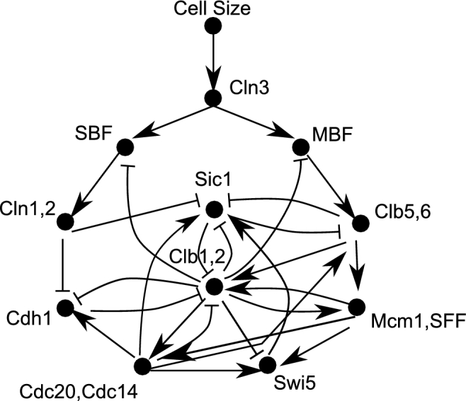
The wiring diagram for the Li threshold model. The network includes cyclins (the G1 cyclins Cln3 and Cln1,2, and the S/M cyclins Clb5,6 and Clb1,2, which all form binary complexes with the kinase Cdk1), the inhibitors of the cyclin/Cdk1 complexes (Sic1, Cdh1, Cdc20, Cdc14), the transcription factors (SBF, MBF, Swi5 and Mcm1,SFF), and the checkpoint Cell Size. Lines with arrowheads represent activators, whereas lines with barbs represent inhibitors. When a yeast cell grows, Cell Size is active (the cell responds to nutrients), leading to the activation of the cyclin Cln3 (G1 phase), which in turn activates by phosphorylation the transcription factors SBF and MBF that activate transcription of the genes of cyclins Cln1,2 and Clb5,6, respectively. Clb5,6 (S phase) activate by phosphorylation the transcription factors Mcm1,SFF that activate transcription of Clb1,2, which continue to promote by phosphorylation the activation of Mcm1,SFF and the inactivation of SBF. Mcm1, SFF also activates transcription of Swi5, which in turns activates transcription of Sic1 that binds to, and inhibits the activity of, the cyclins Clb5,6 and Clb1,2. Cln1,2 and all Clb cyclins phosphorylate and inactivate Sic1, and Clb1,2 (entry into M phase) phosphorylate Swi5 to prevent its entry into the nucleus and inactivate Sic1 transcription. Clb1,2 phosphorylate and activate Cdc20,Cdh1 and Cdh1, which in turn degrades and inactivate Clb1,2 itself (exit from M phase), thus promoting activation of Sic1 (G1 phase). For modeling purposes, the kinase Cdk1, partner of both Cln and Clb cyclins, is not indicated in the network because its activity is driven by the cyclins. Adapted from Li et al. (2004).

The state space—the set of all possible states of the system—of this network has seven fixed points, one of which is consistent with the G1 phase of the cell cycle: the cyclin/Cdk1 inhibitors Sic1 and Cdh1 are active while all other nodes are inactive. This definite state space is referred to as an attractor, a collection of states which is closed with respect to the trajectory, and where each state is visited infinitely often (see Supporting Information for details about the basics of logical modeling). The trajectory that has as its initial condition the G1 fixed point—with the exception of the node Cell Size, which is the only checkpoint always active, indicating that the critical cell size has been reached—models the activity profile of the cell cycle and converges to the G1 fixed point. This trajectory, given in Table 1, verifies that some basic aspects of the cell cycle are representable in a model by using the simplest possible assumptions. Of the seven fixed points, or attractors, only the G1 attractor represents an observable biological state. The others are deemed spurious. However, the basin of attraction—the collection of initial conditions whose trajectories arrive at the attractor—of the G1 attractor is by far the largest. Of the 2048 states in the state space, the basin of attraction for the G1 attractor consists of 1764 states, while the next largest one consists of 151 states (Li et al.2004). This indicates that, for the vast majority of initial conditions, the trajectory will converge to the G1 attractor. Furthermore, it is argued that there is a large overlap between trajectories in this basin of attraction and, thus, there is a ‘convergence of trajectories’.

Table 1.

The trajectory leading to the G1 attractor in the logical cell cycle models.

Time	Cell Size	Cln3	MBF	SBF	Cln1,2	Cdh1	Swi5	Cdc20,14	Clb5,6	Sic1	Clb1,2	Mcm1,SFF	Phase
0	1	0	0	0	0	1	0	0	0	1	0	0	Critical Size
1	0	1	0	0	0	1	0	0	0	1	0	0	Start
2	0	0	1	1	0	1	0	0	0	1	0	0	G1
3	0	0	1	1	1	1	0	0	0	1	0	0	G1
4	0	0	1	1	1	0	0	0	0	0	0	0	G1
5	0	0	1	1	1	0	0	0	1	0	0	0	S
6	0	0	1	1	1	0	0	0	1	0	1	1	G2
7	0	0	0	0	1	0	0	1	1	0	1	1	M
8	0	0	0	0	0	0	1	1	0	0	1	1	M
9	0	0	0	0	0	0	1	1	0	1	1	1	M
10	0	0	0	0	0	0	1	1	0	1	0	1	M
11	0	0	0	0	0	1	1	1	0	1	0	0	M
12	0	0	0	0	0	1	1	0	0	1	0	0	G1
13	0	0	0	0	0	1	0	0	0	1	0	0	Fixed G1

To understand the origins of these features, Li et al. compared the structural properties of their model to random threshold networks with the same number of nodes and edges as well as to networks found by structurally perturbing the cell cycle network. Having a fixed point, or attractor, within such a large basin of attraction, and having many overlapping trajectories is specific to the cell cycle network as compared to random networks with a similar structure. Furthermore, these features are fairly well preserved when making small perturbations to the structure of the cell cycle network, e.g. deleting or adding an edge, or switching an edge between an activator and an inhibitor. This later stability, however, appears to be common to all threshold networks of sufficient size. Li et al. (2004) concluded that this cell cycle logical network is robustly designed. Analysis aside, it is most provocative that a qualitative representation of the cell cycle may be discovered in such a simplistic model. It suggests that the correct ordering of cell cycle events may be determined by an overall logical structure as opposed to the details and mechanisms of specific interactions. Thus, the challenge is to find the appropriate balance between abstraction and specificity, in order to allow construction of computer models that are useful to biologists.

The Fauré and Irons models

The models presented by Thieffry and colleagues (Fauré et al.2009) and Irons (Irons 2009) are intended to be a more realistic representation of the yeast cell cycle. Both models have more nodes and abandon the threshold logic. The update functions for each node are built by summarizing the literature of interactions involving a given node into its update function. Both models incorporate phenomenological nodes, such as a node to indicate whether a cell has initiated budding or has entered cytokinesis. These nodes are also used to incorporate checkpoints. For example, in the Irons model, the DNA damage checkpoint is modeled by fixing the node S/MBF to zero, as Rad53—kinase required for cell cycle arrest upon DNA damage—has phosphorylated the transcription factor Swi6 and prevented the formation of SBF (indicating the Swi4/Swi6 complex) and MBF (indicating the Mbp1/Swi6 complex). For this network, the main attractor, a fixed point, corresponds to a state where Cln3, CKI and Cdh1 are active and all other nodes are inactive. This is the profile of a cell that has been arrested in the G1 phase, consistent with the main attractor found by Li et al.

In order to verify the verisimilitude of these models with the Li model, both authors investigate several mutant phenotypes. It is generally assumed that a knockout may be modeled by setting the corresponding node to zero and changing its update function so that it remains inactive. The models of Fauré and Irons find a qualitative agreement between many model mutants and the corresponding experimental phenotypes. For example, the double mutant swi4Δswi6Δ is known to arrest in the G1 phase (Nasmyth and Dirick 1991). The Irons model incorporates these two proteins into a single node S/MBF whose activity indicates formation of the transcriptional complexes SBF and MBF. Thus, this double mutant is modeled by fixing the node S/MBF to zero. The model finds an attractor with a G1 profile whose basin of attraction consists of 64% of the state space, thus indicating that the model arrests in this cell cycle phase (Irons 2009). Notice that, within the model, there is no difference between this mutant behavior and that of the DNA damage checkpoint. Similar analysis has been performed by Thieffry and colleagues for a vast collection of mutants (Fauré et al.2009). The difference between the two models can be underlined in light of how they implement thresholds into the network logic. The Irons model addresses the variety of time scales among the network reactions by using dummy nodes—empty templates to build new nodes later—to allow for delayed activation or deactivation. These delays can be interpreted in several ways, such as a requirement of an input to reach a threshold or to enforce a sustained activation. With a similar idea, in the Fauré model some nodes follow the binary, Boolean logic, while a range of values are assigned to others. Furthermore, the Fauré model employs a semisynchronous updating scheme referred to as priority classes. That is, most nodes in the network are updated at the same time, or synchronously, however, several of the phenomenological nodes are given priority. For example, if the state of the network is such that the node CYTOKINESIS is active, then this occurs before the update of other nodes (Fauré et al.2009). While both models are built from modules governing individual cell cycle phases, the update function receives more attention in the Fauré model.

The question remains, are these models an improvement of the Li model, and do they provide insights that may inspire further experimentation? In Irons’ study, both the wild type and all viable model mutants are represented by a single attractor. Assuming that the spurious attractors in the Li model do not represent unknown cell types, this is an improvement. In addition, the Irons model shows that the existence of a single attractor is preserved in the absence of the delays that are incorporated into the model. As accurate results derive from (i) a more realistic logic and (ii) a more realistic interpretation of checkpoints, both the Fauré an and Irons models represent an advancement of the Li model. Furthermore, they show that the general order of cell cycle events is well represented by using the synchronous updating scheme. The analysis of mutants in both models does however lead to interesting questions. For example, the swi4Δswi6Δ mutant modeled by Irons has more than one attractor. It seems unlikely that the new attractor represents a real cell type; however, understanding how the network shall be modified to ensure that for this mutant only the G1 attractor is found may lead to new insights. It should be noted that Fauré's mutant analysis is compared to the outcome of the differential equation model for the cell cycle developed by Chen et al. (2004). For example, the latter model shows that the quadruple mutant cln1Δcln2Δcln3Δcdh1Δ arrests in telophase while in the Fauré model it maintains the appropriate order of cell cycle events. Interestingly, the behavior of this mutant is inferred by Chen et al. by assuming that its behavior is similar to yet another mutant (see mutant documentation at http://mpf.biol.vt.edu/research/budding_yeast_model/pp/tyson.php#). While inferring behavior of mutants is a common practice, for the most effective use of mathematical models modelers and the experimenters shall be working together to address yet unknown phenotypes. An example is given by the work of Chasapi et al., where the back and forth between models and experiments lead to a prediction of a counterintuitive mutant phenotype in the fission yeast Schizosaccharomyces pombe which was then validated experimentally (Chasapi et al.2015).

The Barberis model: from a kinetic model to the binary logic

Differently from the aforementioned modeling efforts, the model presented by Barberis and colleagues aims to capture cell cycle dynamics with a minimal set of components. Specifically, the model derives from a previous work of the authors, where a kinetic model was used to predict a novel role for the CKI Sic1, inhibitor of the Clb/Cdk1 complexes active from S-through-M phase (Barberis 2012), in coordinating the timely oscillations of waves of Clb cyclins throughout cell cycle progression (Barberis et al.2012). This model was converted to a Boolean logic, where a prior knowledge network (PKN) with four nodes—comprehending the cyclins Clb5, Clb3 and Clb2, and the CKI Sic1—was generated (Linke et al.2017) incorporating the novel interactions found experimentally (Barberis et al.2012). The wiring diagram is shown in Fig. 2. The authors generated different versions, of variable complexity, of the network where all possible interactions (edges) among the nodes were tested for reproducing qualitatively the oscillatory behavior observed for both Clb cyclins and Sic1 (Zachariae and Nasmyth 1999). The interactions considered (either positive or negative) include one, two, three or four nodes that may influence the activation/inhibition of other nodes. Starting from all possible edges (640), 36 minimal models were generated that were able to reproduce the Clbs/Sic1 oscillatory behavior of a wild-type cell as well as definite Sic1 mutants. Specifically, an attractor was found with the four nodes oscillating in wild type and SIC1 overexpression, and a steady state with all Clb cyclins active in a sic1Δ strain, as experimentally observed (Barberis et al.2012). After simulating the 36 models with SQUAD, a tool that converts logical attractors to ODEs (Di Cara et al.2007), six of them reproduced the Clbs/Sic1 timely oscillations, with sic1Δ loosing Clb oscillations, and SIC1 overexpression delaying the formation of Clb waves. Among these six models, only two were able to match the experimental profile of CLB2 overexpression (Linke et al.2017). Intriguingly, regardless of the number of interactions within these two models, a common, novel regulatory design is identified that connects the three Clb cyclins, which allows for their timely occurrence in a wave-like fashion. That is, all Clb/Cdk1 complexes phosphorylate the transcription factor Fkh2 by a linear regulation, where Fkh2 in turn transcribes for both CLB3 and CLB2 genes, thus coordinating the timely appearance of waves of Clb cyclins (Linke et al.2017).

Figure 2.

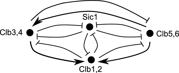
The wiring diagram for the model of Barberis and colleagues. The network includes the S cyclins Clb5,6 and the G2/M cyclins Clb3,4 and Clb1,2, which all form binary complexes with the kinase Cdk1, and the inhibitors of the Clb/Cdk1 complexes Sic1. Lines with arrowheads represent activators, whereas lines with barbs represent inhibitors. In G1 phase, all Clb cyclins are inhibited by Sic1. When Sic1 is degraded and inactivated at the G1/S transition, Clb5,6 (S phase) promote the transcription of CLB3 and CLB2 genes, thus activating both Clb3,4 (G2 phase) and Clb1,2 (M phase) through phosphorylation of the transcription factor Fkh2. Clb3,4 also promotes the transcription of CLB2 gene through Fkh2 phosphorylation. All Clb cyclins phosphorylate and inactivate Sic1. Furthermore, the cyclins that are activated later inhibit the ones activated earlier: (1) Clb1,2 phosphorylate and activate Cdc20 and Cdh1, which in turn degrades and inactivate Clb5,6 and Clb3,4, and (2) Clb3,4 inactivate Clb1,2, thus promoting activation of Sic1 (G1 phase). For modeling purposes, the kinase Cdk1, partner of Clb cyclins, is not indicated in the network because its activity is driven by the cyclins. Adapted from Linke et al. (2017).

Altogether, the logical structure of the cell represented by the models described above is sufficient to provide a blueprint for ordering the rise and fall of cyclins and CKIs—or, wider, of cyclin/Cdk1 competitors—throughout the cell cycle. These models may then be used to make falsifiable predictions, which will help to evaluate the validity of model assumptions, although they represent a simplistic view of the cell cycle processes.

ROBUSTNESS OF THE CELL CYCLE STRUCTURE

Tan and colleagues already suggested that the size of the basin of attraction in the state space graph is a measure of robustness (Li et al.2004); that is, biological systems have to be robust to perturbations to adapt to stress, environmental changes, etc. However, other notions of robustness have been explored. Horowitz and colleagues sought to find out how robust the Li model's cell cycle trajectory and the G1 attractor are to deviations from a synchronous update (Mangla, Dill and Horowitz 2010). They investigated every path in the asynchronous state space graph that starts at the excited G1 state (time 0 in Table 1) in order to determine if each of them ends at the G1 attractor, by using the model checker software NuSMV (Cimatti et al.2000). Mangla et al. referred to a non-biological (non-realistic) update in the trajectory as a hazard; by diagnosing each such hazard, the authors propose changes to the logic of the network in order to eliminate all of them. For example, in the Li model, there is a path where the degrader Cdc20 is deactivated before the activation of the degrader Cdh1, leading the cell cycle to halt. Mangla et al. revised the model so that Cdc20 negative self-regulation was replaced by a Cdh1-mediated negative regulation. Also, Clb2 is expanded beyond a Boolean variable to take on values 0, 1 or 2, and the logic was appropriately changed. Furthermore, Cln3 negative self-regulation was replaced with the inhibition by SBF and MBF. By introducing these modifications, the authors generate a logical network where every path in the asynchronous state space graph starting at the excited G1 state ends at the G1 attractor (Mangla, Dill and Horowitz 2010). A number of these changes also appear in other models. For example, the model of Ding and Wang (2011) includes Cdh1 as a negative regulator of Cdc20. These examples show how the analysis of logical models can be used to elucidate new regulatory interactions between species in a genetic network.

Shin and colleagues brought this analysis further, investigating whether each path in the asynchronous state space graph starting at the G1 excited state ended at the G1 attractor was biologically relevant (Hong et al.2012). In particular, the authors identify in the Li model and Mangla's amended model trajectories where Cdc20 is activated before the activation of Clb2. Therefore, the models were revised by adjusting the weights in several of the logical functions (all of these networks use threshold functions): assigning to a number of nodes variable activity levels (for example, Swi5 = 0, 1 or 2), and adding new interactions (for example, a positive feedback between Clb2 and Mcm1). The result is a logical threshold network where the evolution from the excited G1 states to the G1 attractor actually models the evolution of the cell cycle, regardless of the order used to update the nodes (Hong et al.2012). Furthermore, the authors perform a similar attractor analysis as in the work of Li et al. and find similar results: a G1 attractor with a very large basin of attraction.

Instead of a synchronous update, Goles, Montalva and Ruz (2013) define an update schedule, that is, the order in which the nodes are updated. With a given schedule, the network is updated deterministically. The authors develop tools specific to threshold logical networks that account for a vast number of update schedules to consider—even for a small network such as the one of Li et al.—and conclude that the G1 attractor of the Li model is a fixed point for every update schedule, and has the largest basin of attraction (Goles, Montalva and Ruz 2013).

Braunewell and Bornholdt (2007) develop a more elaborated analysis on the Li model, as the logical network is converted to a system of differential equations, and show that it is robust to small stochastic variations in the update order. As noted by Mangla, Dill and Horowitz (2010), the cell cycle itself is not robust such that any order of activations is permissible; thus, a fully asynchronous network to model the cell cycle may be as questionable as using a fully synchronous network. How this relates to the actual biology of the cell cycle is unclear. It is true that in general the difference between synchronous and asynchronous can be quite dramatic. Strikingly, the fact that the yeast cell cycle logic seems to constrain these differences may result from evolutionary pressures; evolvability may in fact select robust and flexible processes that can adapt to changes in environmental cues (Kirschner and Gerhart 1998) that may impinges on the functionality of the cell.

The models above provide insights in the understanding of those nodes that are key to the ordering of cell cycle events. Tang and colleagues address this question by investigating the feature(s) that a (threshold) logical network must have in order to reproduce the cell cycle trajectory found by Li et al. (Lau, Ganguli and Tang 2007). By enumerating the threshold networks with 11 nodes, the authors found that 10 interactions in the Li network are required to observe the cell cycle trajectory. They are as follows: (i) activation of SBF by Cln3; (ii) activation of MBF by Cln3; (iii) activation of Clb1,2 by Clb5,6; (iv) activation of Mcm1/SFF by Clb5,6; (v) inhibition of Sic1 by Cln1,2; (vi) inhibition of Cdh1 by Cln1,2; (vii) inhibition of Clb1,2 by Sic1; (viii) inhibition of Cdh1 by Clb1,2; (ix) activation of Mcm1/SFF by Clb1,2; (x) activation of Swi5 by Cdc20/Cdc14. The networks that contain these interactions have, on average, larger basins of attraction and, correspondingly, fewer attractors. Boldhaus and Klemm (2010) took a similar approach by analyzing the structural properties of the ensemble of logical threshold networks with 11 nodes that realize the cell cycle trajectory found by Li et al. Even among those networks that generate the cell cycle trajectory, the Li network stands out: it has fewer interactions, and the basin size of the G1 attractor is actually smaller than the average network that produces the cell cycle trajectory.

Essentially, all the modeling efforts presented here support the structure of the Li model, and investigate only logical networks with threshold functions. The models of Fauré and Irons abandon this assumption and, thus, the analyses do not extend to those models. As highlighted by Glass and colleagues, the structure of the genetic networks of the budding yeast cell cycle determines robust dynamics (Perkins, Wilds and Glass 2010); thus, it represents a scaffold that may integrated with regulatory layers that crosstalk together to drive cellular functions.

Implementation of stochasticity

Further analyses of the Li network have been performed by incorporating stochasticity (Zhang et al.2006a,b; Ge, Qian and Qian 2009; Lee and Huang 2009), with the aim to understand the robustness of the cell cycle network with respect to noise in the update function. Zhang et al. and Lee and Huang extended the Li model to an irreducible time-independent Markov chain. To do this, the authors assigned a probability, or noise, ρ so that a given node in the network would follow the defined update function with probability 1−ρ while it would update randomly with probability ρ. The details of how these modeling efforts introduced this noise differ, but the analysis that follows is similar, as both examine the details of the steady-state distribution of Markov chain (Zhang et al.2006a,b; Lee and Huang 2009). In both studies, the state of maximum likelihood corresponded to the G1 attractor identified in the Li model, and the most likely trajectory corresponded to the Li's cell cycle trajectory. Furthermore, the studies also found that a phase transition occurs: when the noise passes a critical level, the steady-state distribution of the Markov chain no longer favors the G1 attractor, nor the cell cycle trajectory, and the network behavior becomes essentially random.

In Ge et al., the same network built by Zhang et al. was considered, but a more sophisticated analysis was performed by using circulation theory for Markov chains (a topic beyond the aim of this work). Even in the context of this analysis, a similar result was found: the Li network shows remarkable robustness to noise in the network update rules (Ge, Qian and Qian 2009). Stoll et al. also study the Li network with perturbation by using the stationary distribution of the corresponding Markov chain. In addition, checkpoints are added externally. Using concepts from information such as entropy and mutual information, the authors show that several essential interactions, including all of the negative self-regulations, contribute to the proper behavior of the Li network with perturbation (Stoll, Rougemont and Naef 2006). Interestingly, a different set of regulatory interactions was found as compared to Lau, Ganguli and Tang (2007); in addition, a significant amount of symmetry was observed in the Li network that contributes to its stability.

Most of the analyses presented in this section seek to identify the origins of different types of robustness, or to inquiry into the prudence of particular modeling choices. In some ways, these questions overlap and arise naturally in the context of logical modeling. The analyses presented are in line with one of the basic conclusions of Irons: ‘the exact timing of events, and the order in which the nodes update, does not alter the fundamental behavior of the system’ (Irons 2009). While there are features common to many models as well as results from different analyses that point to common features, it is clear that the details of certain choices are critical to understand from a biological point of view, such as the choices made when defining the update functions. As noted by Fauré et al., ‘detailed analysis of the mutants reveals that, in some cases, incorporation of refined information about expression … may be necessary to fully reproduce some properties of the system’ (Fauré et al.2009). Investigating the robustness of the cell cycle trajectory with respect to update order of deletion of edges has a natural interpretation in the cell, such as the timing of interactions, explanation of deletion mutants, and so on. However, the robustness being measured by incorporating noise in the update function should somehow be related to the stochasticity inherent in gene expression (Rao, Wolf and Arkin 2002; Raj and van Oudenaarden 2008). The effect of stochastic gene expression as perturbation in a logical network should be explored in more detail.

ADVANCES IN LOGICAL MODELING: PREDICTING BIOLOGICAL SCENARIOS

Recently, several studies have been presented that include a more detailed verification of the models aforementioned, make detailed predictions or combine predictions with detailed experimentation. The three studies that will be presented in the following, Todd and Helikar (2012), Alcasabas et al. (2013) and Rubinstein et al. (2013), have their foundations in the work of Li, Fauré or Irons. Todd and Helikar (2012), while adapting their model from the one of Irons (Irons 2009), investigated the cell cycle logical network as a Markov chain where stochasticity is not interpreted as noise but as continuous activity level. Specifically, if a node has probability p of being active, then this probability is interpreted as its activity level. While the study does not make direct predictions or suggest specific experiments, it demonstrates that logical information can be used to derive continuous activation curves for the species represented in the model. Furthermore, in the study of Todd and Helikar, the time is incorporated only relative to the cell size. This is a significant departure from the notion that the steps in a trajectory of a logical network are the only way that time can be incorporated. As previously noted, several authors investigate Markov chain versions of the yeast cell cycle network. In those studies, stochasticity was included by using the concept of a noise; as such, the notion of an attractor was no longer applicable. However, the results of Todd and Helikar support the idea that irreducible sets of states, also called ergodic sets, of a Markov chains are the natural extension of the attractor as previously noted (Ribeiro and Kauffman 2007). The model, unlike a traditional logical network, is not autonomous. The model contains input nodes that stand for external conditions, the cell size in particular. Thus, the authors show that the activities of the primary cyclins are highly robust to variations in what they term ‘cell size signal’, i.e. the cell cycle network is robust to variations in the external environment. A qualitative similarity was observed when comparing the analytically calculated results of Todd and Helikar with the experimental ones found by Cho et al. regarding the mRNA transcript profile of the network components throughout cell cycle progression (compare Cho et al.1998 and Todd and Helikar 2012). Furthermore, the model reproduces a secondary activation for the G1 cyclins that occurs later in the cell cycle, as observed experimentally (Cho et al.1998). In addition, the model reproduces qualitatively experimental results of Charvin et al. (2010), showing that the checkpoint START driving cells through the G1/S transition is reversible without a positive feedback loop involving Cln1,2.

The work of Oliver and colleagues is based on the Fauré model and employs a logical model to predict how variation in the copy number of genes influencing growth rate may modulate progression throughout the mitotic cell cycle. The authors use the standard interpretation of time as steps in a trajectory but, similar to the work of Todd and Helikar, they use stochasticity to model node activation. To test the effect of growth, sequential deletions of alleles in tetraploid yeast cells were conducted, with mutants expressing 0%, 25%, 50% and 75% of the wild-type dosage, corresponding to 0, 1, 2 and 3 gene copies (Alcasabas et al.2013). The gene dosages were then modeled by probabilities. That is, if a gene is to have 25% of the wild-type dosage, then the corresponding node is assumed to take the value 1 for the 25% of the time, and the value 0 for the remaining 75% of the time. As the model is stochastic, attractors are not well defined, with the exception of the wild-type or the homozygous deletion mutants (0% and 100%, respectively). In the wild-type model (a direct descendent of the Fauré model), the trajectory starting in an excited G1 state ends at a stationary G1 state and, as with the other models, the activations of the species match that expected in the course of the cell cycle. This trajectory has 31 steps and, thus, establishes a time against which the behaviors of deletion mutants may be compared (Alcasabas et al.2013). In the stochastic model, trajectories will differ over each iteration. To determine the number of cell cycles that occur over a given trajectory, the activation and deactivation of the nodes START, CYTOKINESIS and MASS are verified. The authors then calculate the length of individual cell cycles and compare the length of the various deletion mutants to the wild-type length of 31 steps. The model predicted a phenotypic difference in growth rate between deletion mutants with low copy numbers for CLB1 and CLB2 cyclin genes—which regulate the timing of cell division together with the kinase Cdk1—that was observed experimentally (Alcasabas et al.2013). Furthermore, the model shows that different dosages of the kinase Cdk1 can result in phenotypic variation. In fact, as CDK1 gene dosage decreases from the wild-type levels to 50% of that level, an increasing number of cells accumulate in the G2 phase, about 2.5 times the wild-type level. Noticeably, this is consistent with a connection between gene dosage and phenotypic variation (Ouahchi, Lindeman and Lee 2006). These results suggest that novel predictions can emerge from logical modeling. However, the authors also identify several deviations between model predictions and experimental results. In particular, the growth rate predicted for the low copy numbers of SWE1, negative regulator of the Cdk1 kinase, was slower as compared to the experimental observation (Alcasabas et al.2013).

Kassir and colleagues develop a threshold logical model where the nodes take values in {0, 1, …, 9}, and it can be considered to descend from the Li model. However, this model is significantly larger, containing 65 nodes that represent RNA, proteins and cellular events (Rubinstein et al.2013). The authors show that when the model starts at an excited G1 state the system falls into an attractor that, as in the Li model, mimics the activation levels of the nodes. Furthermore, the model is able to reproduce the behavior of several mutants and the cell cycle response to nitrogen depletion (Rubinstein et al.2013). Strikingly, the model is able to make detailed predictions. It has been suggested that the transcription factor Hcm1 is a Cdk1 target (Ubersax et al.2003); thus, the authors have examined three possible ways by which Hcm1 can be activated by phosphorylation by the kinase complexes: (i) Cln3/Cdk1, (ii) Cln1/Cdk1 and (iii) Clb5/Cdk1. The model predicts that if Cln3/Cdk1 activates Hcm1, there is a premature decline in the transcription of the CLB2 cyclin gene during the S phase (Rubinstein et al.2013). Contrarily, if Cln1/Cdk1 or Clb5/Cdk1 activates Hcm1, the basic behavior of the cell cycle is observed; a simulation of the response to pheromone treatment suggested that Cln1/Cdk1 is more likely the activator of Hcm1.

For each of the three models presented in this section, scale is a significant challenge. While Helikar and Todd characterize the entire state space of their model, such computations are not feasible for systems that are substantially larger. On the other hand, the models of Alcasabas et al. and Rubinstein et al. are so large that the full state spaces can hardly be explored. For example, the state space of the Rubinstein et al. model, which contains 65 nodes, has about as many states as there are seconds in 1.6 trillion years (2⁶⁵ states). Perhaps more incredibly, a cyclic attractor is found at all.

More recently, Barberis and colleagues provide another example of a sophisticated use of modeling and traditional bench biology (Linke et al.2017). In particular, a simple logical model containing four nodes (Fig. 2), each representing a cell cycle phase, was used to inform the experimentation and to explain the results. Two types of logical modeling were employed: (i) a multi-valued model satisfying the behavior of known experimental conditions (Barberis et al.2012) that was analyzed using GenYsis, a tool developed to reproduce the logical attractors (Garg et al.2008); and (ii) a stochastic exploration of the asynchronous state space using Gillespie's stochastic sampling algorithm using the software MaBoSS (Stoll et al.2012). The model of Barberis and colleagues was validated against the Clb2 overexpression phenotype, showing that an increase of Clb2 level upon a certain threshold leads to a reduction in the number of Clb waves (Linke et al.2017). This outcome is compatible with the inhibition of mitotic exit, as experimentally observed (Cross et al.2005). Furthermore, the model predicted that waves of expression of mitotic CLB cyclin genes are the result of cyclin/Cdk1-dependent linear regulation on the transcription factor Fkh2 (Linke et al.2017), which is the main regulator of CLB2 transcription (Koranda et al.2000; Kumar et al.2000). The contribution of the logical model, based on the minimal number of interactions needed to capture the information flow of the Clb/Cdk1 network, is 2-fold: first, it captures the current knowledge of the regulation among Clb cyclins and the Clb/Cdk1 inhibitor Sic1; second, it predicts and independently verifies the interactions—proven experimentally—among the nodes without assuming any prior regulatory knowledge, but only by reproducing the expected behaviors known from the literature. Strikingly, the model was able to predict a novel principle of design in cell cycle regulation, i.e. a linear transcriptional cascade of activation of mitotic CLB genes that is required to reproduce the sequential appearance of waves of Clb cyclins (Linke et al.2017). This continue iteration among modeling and experimentation, typical of the systems biology circle, proves to be increasingly successful to provide a rational explanation of cellular functions by identifying regulatory mechanisms previously unraveled.

A summary of the logical models of cell cycle regulation and their properties is presented in Table 2. All of the models discussed above remain in the qualitative regime and may be predictive; however, they are divided in explanatory or predictive, according to the use they have been built for.

Table 2.

Logical models of cell cycle regulation and their properties.

Model	Nodes	A/Synchronous	Stocastic/Deterministic	Use
Li et al.	12	Synchronous	Deterministic	Explanatory
Irons	18	Synchronous	Deterministic	Explanatory
Fauré et al.	27	Mixed	Deterministic	Explanatory
Todd and Helikar	20	Synchronous	Stochastic	Explanatory
Rubinstein et al.	67	Synchronous	Deterministic	Predictive
Alcasabas et al.	52	Mixed	Stochastic	Predictive
Zhang et al.	12	Synchronous	Stochastic	Explanatory
Linke et al.	4	Synchronous	Deterministic and Stochastic	Predictive

THE CHALLENGE: BINARY LOGIC IN MULTI-SCALE MODELING OF CELLULAR REGULATION

The physiological responses of a cell are governed by a flux of information that is integrated through complex processes. Cellular communication, metabolism, signaling networks, gene regulation and cell cycle machinery have to be tightly regulated to sustain cellular homeostasis (Gonçalves et al.2013). Whereas modeling approaches in the past have focused on cellular processes delimited by spatiotemporal scale or function, they are now increasingly being integrated (Kitano 2002). The cell cycle models described above often implicitly accounted for multiple scales and functions. Boundary conditions such as cell cycle checkpoints, cell size and other phenomena are summarized in phenomenological nodes, making assumptions about processes carried out by other functions occurring at different spatial and/or temporal scales. Examples are the models of Irons (Irons 2009) and Fauré (Fauré et al.2009), which contain phenomenological nodes representing budding and cytokinesis, and the model of Li (Li et al.2004), which contains a phenomenological node accounting for the cell size that a cell has reached when the G1 Cln3/Cdc28 complex approaches its critical level. Even so, these models cannot be regarded as multi-scale, as multi-scale models have to account for processes and functions on different temporal and spatial scales in an explicit way. Furthermore, multi-scale models must carry additional information about the merged subsystems not present in the exploration of the independent systems. Thus, information must be carried over borders of spatiotemporal scales (Walpole, Papin and Peirce 2013).

As elements in functional systems differ in the way they are logically connected to each other and in the way information is gathered about them, no single formalism is able to correctly and conveniently model all different functions and scales. To illustrate, metabolism is usually modeled with stoichiometric models employing a constraint-based approach such as Flux Balance Analysis (FBA, see below and Supporting Information for details), although smaller subsystems can be represented more accurately by using kinetic models (Gombert and Nielsen 2000; Lewis, Nagarajan and Palsson 2012). Models of signaling networks use a wide range of formalisms including Bayesian networks, logical, stochastic and rule-based models, sets of ordinary differential and partial differential equations (ODE, PDE), constrained fuzzy logic (Terfve and Saez-Rodriguez 2012; Gonçalves et al.2013). Cell networks and tissues are often modeled using an agent-based method (Walpole, Papin and Peirce 2013). For an oversight of the common use of modeling formalisms for different scales, see Walpole, Papin and Peirce (2013). An up-to-date oversight of all popular modeling, formal analysis approaches and tools to carry them out can be found in Bartocci and Lió (2016).

There are several explicit difficulties in bridging the gap between individual biological subsystems and scales. Often mechanistic knowledge about the connection between different subsystems is lacking, as it is the case for the interconnection between metabolism and cell cycle in yeast (Cai and Tu 2012). Furthermore, combining two different formalisms might lead to inconsistencies. For example, when stochastic and deterministic approaches are used to model the same reaction, completely different phenomena can be observed, as illustrated in Qu et al. (2011). Finally, finding the right relative temporal scale for submodules can be challenging. A successful example of bridging different temporal scales and biological process is provided by Papin and colleagues, who developed a model of budding yeast based on an FBA variant called integrated dynamic FBA (idFBA, see below) (Lee et al.2008). In this study, the authors integrate metabolism, signaling and gene regulation by coupling fast and slow reactions, to generate quantitative, dynamic predictions.

To date, very few efforts have been made to create multi-scale integration models of cell cycle with other cellular or intercellular processes. Notably, Covert and colleagues constructed a whole-cell model of the human pathogen Mycoplasma genitalium which simulates processes, among others DNA replication and cell division, in a chronology that resembles events occurring throughout its life cycle (Karr et al.2012). However, the intricate interplay of cyclins, CKIs and transcription factors is not represented in their attempt. To our knowledge, the only case in which the cell cycle, represented by a logical model, has been integrated in a multi-scale fashion is the model for avascular tumor growth by Jiang et al. (2005). Integration of other subsystems, such as gene regulation with metabolism, might provide insights that can be used to integrate the cell cycle in its wider environment. Table 3 presents an overview of modeling approaches that integrate binary logic with other modeling strategies in budding yeast as well as in other organisms. In the following, we provide an overview of the efforts that have been made to employ logical modeling in multi-scale models, where the binary logic has been used as the only strategy, or where stoichiometry, kinetic and hybrid modeling strategies and data-driven models have been integrated with the logical modeling. Furthermore, approaches currently under development will be presented, where appropriate. These may serve as basis for the generation of multi-scale models in budding yeast.

Table 3.

Computational efforts integrating binary logic with various modeling strategies.

Modeling strategy	Formalisms	Subsystems	Source
rFBA (regulatory)	Boolean, FBA (constraint)	Metabolism, gene regulation	Covert and Palsson (2002)
srFBA (steady-state regulatory)	Boolean, FBA (constraint)	Metabolism, gene regulation	Shlomi et al. (2007)
iFBA (integrated)	Boolean, FBA (constraint), ODE	Metabolism, gene regulation, signaling	Covert et al. (2008)
idFBA (integrated dynamic)	Boolean, FBA (constraint)	Metabolism, gene regulation, signaling	Lee et al. (2008)
Multi-scale tumor model	Boolean, ODE, Discrete lattice Monte Carlo	Cell cycle, metabolism, cellular responses (growth, volume, proliferation)	Jiang et al. (2005)
Hybrid systems theory	Boolean, ODE	Gene regulation, signaling	Sneddon, Faeder and Emonet (2011); Tenazinha and Vinga (2011); Ryll et al. (2014)
Hybrid modeling	Boolean, PLDE	Cell cycle	Singhania et al. (2011)
Hybrid modeling (GESSA)	Probabilistic Boolean, Stochastic, ODE	Gene regulation, signaling, environmental stimuli	Fertig et al. (2011)
Data-driven model	Boolean, Data-driven (statistical)	Cell cycle, gene regulation, signaling	Melas et al. (2011)
Boolean–Boolean extension	Boolean	Gene regulation, signaling	Schlatter et al. (2012)
Boolean–Boolean integration	Boolean	Metabolism, gene regulation	Silva-Rocha et al. (2011)

BINARY LOGIC INTEGRATING REGULATORY LAYERS

In a few cases, multi-scale models are generated by using exclusively a binary logic. De Lorenzo and colleagues bridge the gap between subsystems with an all-Boolean model by creating a regulatory circuit describing a system that combines three levels of regulation: metabolism, transcription factors and gene regulation (Silva-Rocha et al.2011). The authors investigate the mechanisms of m-xylene biodegradation by Pseudomonas putida by integrating conventional regulatory elements—such as transcriptional regulators and sigma factors—alongside with less conventional elements—such as metabolic enzymes, intermediate metabolites and histone-like proteins—and phenomena such as growth and temperature, represented as nodes in a logical network. The presence and/or activity of former elements discretized into Boolean values determines the presence and/or activity of other elements through Boolean functions. As such, the model can account for the fact that enzymes and substrates/products physically or functionally interact with transcription factors. The model was not validated experimentally, and served as a visualization of the knowledge about the m-xylene degradation pathway. By using a similar, all-Boolean strategy, Dandekar and colleagues integrated existing logical models by coupling two logical models of hepatocyte signal transduction: one describing the proliferation/apoptosis pathways within a cell and the other one considering cell–cell interactions (Schlatter et al.2012). The integration between the two models occurs where nodes overlap. Modeling standards for logical models are proposed to ensure smooth model integration between modules.

INTEGRATING BINARY LOGIC WITH STOICHIOMETRY

Constraint-based modeling is a widely adopted approach to study biochemical networks, especially suited for metabolic networks (Gianchandani, Chavali and Papin 2010; Orth, Thiele and Palsson 2010; Lewis, Nagarajan and Palsson 2012). A number of multi-scale models that employ a logical component, integrate it with a FBA component. FBA calculates the flux of metabolites through a constrained network while optimizing for an objective function (often represented by the biomass equation), assuming the system being at steady-state (see Supporting Information). FBA can predict growth rate, production rate of important metabolites and/or changes in metabolite flux due to changing environmental conditions. Since no kinetic parameters are needed for model generation, large networks can be reconstructed and simulated, by imposing a relatively low computational demand and by creating the possibility to run simulations using wide ranges of starting conditions and perturbations. These advantages have led to metabolic models being available for at least 35 organisms (Orth, Thiele and Palsson 2010). However, because FBA is carried out at steady-state, only fluxes can be analyzed and no information about the concentration of metabolites can be retrieved. Furthermore, regulation, either due to genetic or protein–protein interaction, is not intrinsically included in FBA, possibly leading to inaccurate predictions (Orth, Thiele and Palsson 2010).

Regulatory FBA

An integration of logical modeling with FBA has been proposed by Palsson and colleagues (Covert, Schilling and Palsson 2001). The authors have devised a method called regulatory FBA (rFBA) where FBA models may account for gene expression and gene product activity. In rFBA, a constraint-based FBA model is regulated by a Boolean regulatory network. Boolean equations restrict the value of gene transcription to 1 (gene transcribed) and 0 (gene not transcribed); as a consequence, transcription of genes determines the presence (1) or absence (0) of proteins (see Supporting Information for details). Palsson and colleagues have employed rFBA to integrate metabolism with transcriptional regulation in budding yeast (Herrgård et al.2006). The authors have reconstructed a minimal transcriptional network that is regulated by nutrient concentrations. In their model, 55 transcription factors regulate the transcription of 750 metabolic genes based on the concentration of 82 distinct intracellular and extracellular metabolites. A logical network is set so that the metabolites determine the state of a transcription factor, which in turn determines the transcription of a metabolic gene.

rFBA bridges the temporal scales of metabolism and gene regulation by introducing a discretized time step tuned to the scale of protein synthesis and degradation. As the time scale of metabolism is faster (milliseconds to tens of seconds) as compared to the transcriptional regulation (in the order of a few minutes or slower), the quasi steady-state of metabolism can be assumed to occur instantaneously after a new proteome is set. Applications of constraint-based modeling integrated with dynamic and regulatory information have started to be employed in the generation of multi-tissue and multi-scale models of higher organisms (Martins Conde Pdo, Sauter and Pfau 2016).

In the following, we will demonstrate the relevance of constraint-based modeling for incorporating the cell cycle within its cellular context. Specifically, we will show how rFBA methodologies may be integrated with logical modeling to explore the mutual regulatory interactions between cell cycle and metabolism.

Integrated dynamic FBA

Differently from rFBA and iFBA (see below), the integrated dynamic FBA (idFBA) developed by Papin and colleagues represents not only metabolic reactions, but also signaling pathways and gene transcription in a stoichiometric matrix (Lee et al.2008). This strategy converts logical networks describing signaling and gene transcription into a matrix, by using a formalism described by Palsson and colleagues (Gianchandani et al.2006). The idFBA framework, applied to a module of budding yeast that includes a portion of the high-osmolarity glycerol (HOG) response pathway, incorporates 26 reactions among 48 components. It aims to account quantitatively for the production and use of proteins in the cell, and it introduces a cost for the amino acids required for protein production. The integration of signaling with regulation, which occurs on a far slower time scale, with fast metabolism, creates a scale issue. To solve this issue, time is discretized into small steps (see Supporting Information for details).

Another issue within the idFBA methodology lies in the definition of the objective function. To define a relevant objective function, Papin and colleagues use an algorithm that defines objective functions based on network stoichiometry, and selects for relevancy by comparing with experimental flux data (Gianchandani et al.2008). Since the cell cycle is governed by a number of signaling cascades (such as PKA and TOR that regulate response to nutrients, or DNA damage signaling), as well as by gene regulation (in the form of transcription factors) and metabolism (in the form of growth), idFBA may be an interesting strategy to employ for the integration of these regulatory layers.

INTEGRATING BINARY LOGIC WITH KINETICS

Hybrid models, already proposed by Glass and Kaufmann in 1973, integrate discrete (logical) with continuous modeling, thereby opening the possibility to simulate modules that can be best represented with discrete values and modules best described using continuous equations (Glass and Kauffman 1973). Additionally, parts of modules that cannot be fully described using continuous modeling—due to a lack of knowledge on kinetic parameters—can be replaced by discrete modeling techniques (Tenazinha and Vinga 2011). An example is represented by a model of the mammalian cell cycle described by Tyson and colleagues, where the Boolean representation of the cyclins in the Li model is replaced by ODEs (Singhania et al.2011). Additionally, an equation is added to represent the exponential growth and division of the cell over time. The features of the model are the following: (i) Boolean states influence the rate of cyclin synthesis and degradation; (ii) cell growth and division are a function of time; (iii) Boolean states of the transcription factors are dependent only on the cell cycle phase where the cell grows, and not on the state of other transcription factors; (iv) the cell cycle phase is determined by time, cyclin concentration, cell mass or a combination of the former.

Fertig et al. present another example of a hybrid approach, named GESSA (Graphically Extended Stochastic Simulation Algorithm), used for multi-scale modeling by using a Boolean component (Fertig et al.2011). The authors model multi-cell signaling and transcriptional reprogramming by using a Pooled Probabilistic Boolean Network (PPBN) model of cell signaling and a stochastic simulation of transcription and translation model, which responds to a diffusion model of extracellular signals (Fertig et al.2011). The system is applied to simulate the development of Caenorhabditis elegans and predicted phenotypes are compared with the experimental ones. The PPBN model represents an abstraction of the signaling pathway to circumvent high computational cost and the need of parameters, whereas the gene transcription model—which occurs at a longer time scale—is modeled by using the stochastic simulation algorithm originally developed by Gillespie (1976). This allows for the simulation of the generation of transcripts and proteins by a small number of molecules. The diffusion model simulates the behavior of ligands that can diffuse in three dimensions from a constant point source. The three different modules are allowed to run asynchronously; each module has a specified (continuous or discrete) time step after which the organism state is updated, which is used to re-initiate the cell signaling and transcription/translation processes. This allows for a smooth integration of processes active on different temporal and spatial scales. Within the framework, an additional manual specifies how appropriate models can replace the ones used in the paper as examples. Interestingly, the inclusion of a cell cycle model has not been attempted yet.

Another hybrid, multi-scale model is presented by Jiang et al. (2005), and mimics the avascular tumor growth by integrating the G1/S cell cycle transition and growth to the extracellular microenvironment (production of waste, i.e. lactate, and consumption of nutrients, i.e. glucose). At the subcellular level, a Boolean logic regulates the protein network that control the expression of cell cycle proteins; the input for the Boolean network consists of continuous concentrations of different groups of molecules which can be above or below critical thresholds resulting in arrest, quiescence or necrosis. At the extracellular level, concentrations of components are determined by a set of differential equations describing their diffusion, consumption and production. At the cellular level, a lattice Monte Carlo model integrates growth, cell volume, proliferation, death and intercellular adhesion, resulting in a 3D simulation of spherical growth of the tumor cells. To integrate the different time scales, each cell has a clock that determines the cell cycle phase. For each iteration, first the cell lattice is evolved, next the chemical reaction diffusion equations are solved for ¾ h, after which the Boolean network is updated and all cells progress into a new cell cycle phase. Model behavior is compared quantitatively with experimental work in multicellular spheroids (Jiang et al.2005).

Another integrative framework is presented by Klamt and colleagues, where signaling and gene regulatory pathways are linked with metabolic models (Ryll et al.2014). Specifically, an ODE model of hepatocyte metabolism is linked to a logical model of signaling and gene regulation. First, the multiple interfaces between signaling and metabolism were classified. Subsequently, the Boolean network was converted to a system of logic-based ODEs by using the Odefy transformation method (Wittmann et al.2009). The resulting continuous value between 0 and 1 was then fed into the metabolic kinetics. The other way around, the output of the metabolic ODEs was normalized to the values 0 and 1 to feed back into the Boolean network. Finally, parameter values were recalibrated, since the submodules were previously parameterized independently. The model describes qualitatively the switch-like dynamics of hepatocytes in response to nutrients; however, focused experiments have not been performed yet to validate the model.

With the Network Free Stochastic Simulator, NFsim, Emonet and colleagues integrate binary logic and kinetic modeling, where parts of Boolean networks can be replaced for piecewise linear or hill functions as more fine grained knowledge about the system is gathered (Sneddon, Faeder and Emonet 2011). NFsim simulates complex dynamics where a detailed mechanistic knowledge is missing, and overcomes the computational cost associated with biochemical combinatorial issues. The methodology is suitable to model a wide range of systems, which at present include immune system signaling, microbial signaling, cytoskeletal assembly and oscillating gene expression (Sneddon, Faeder and Emonet 2011).

INTEGRATING BINARY LOGIC WITH KINETICS AND STOICHIOMETRY

Integrated FBA

A development of rFBA, called integrated FBA (iFBA), has been proposed by Covert et al. (2008) to integrate binary logic with kinetic and stoichiometric strategies. Specifically, in addition to the Boolean network, a module of the metabolic network for which kinetic parameters are known is replaced by a kinetic model consisting of a set of ODEs (see Supporting Information for details). An advantage of iFBA over rFBA is that the ODE modules contain far more detail than their FBA counterparts, and it enables the calculation of intracellular metabolite concentrations in specific areas of the metabolism where kinetic parameters are known. This is critical for events in which the regulation is depends on internal metabolite concentration. Another advantage of iFBA over rFBA is that it can restrict fluxes to non-zero values that would normally have no flux because they do not contribute to growth or other objective functions. This is especially relevant in the context of the possible integration of the cell cycle with an FBA model, since to define objective functions that will drive flux toward cell cycle proteins without perturbing their dynamics is a challenge. Remarks on multi-scale properties described for rFBA also apply to the iFBA strategy.

INTEGRATING BINARY LOGIC WITH DATA-DRIVEN MODELS

Logical, constraint-based and kinetic models can only be constructed with the knowledge about the connectivity between their components (bottom-up approach). In contrast, data-driven models provide a top-down approach for which the knowledge about the connectivity among entities is not always needed. For example, if gene expression data are used to constrain a metabolic model, it is sufficient to know how genes relate to the metabolic reactions (connectivity), but not which are the intermediate steps or the biological processes (mechanistic knowledge). An example of a data-driven approach combined with logical modeling is a method developed by Alexopulos and colleagues that integrates logical models of signaling pathways, optimized with high-throughput phosphoproteomic data, to cellular responses such as growth, death, differentiation, cytokine secretion and gene expression in order to investigate cellular responses in hepatocellular carcinoma (Melas et al.2011). A multi-linear regression algorithm was employed to generate regression coefficients that serve as weights for the connection of key phosphoproteins with cellular responses. The approach was validated by comparing the simulations with hepatocyte cellular responses and phosphoprotein activity. One issue, often mentioned, with multi-scale modeling is the lack of knowledge about submodule interfaces. Integrating logical and data-driven models provides support to fill the gap between data from observable cell features and detailed networks resulting from mechanistic knowledge.

PERSPECTIVES: INTEGRATING BINARY LOGIC WITH STOICHIOMETRY TO ADDRESS THE MUTUAL REGULATION BETWEEN CELL CYCLE AND METABOLIC YEAST NETWORKS

Recent interest has focused on the regulation between cell cycle and metabolism, both in budding yeast (Alberghina et al.2012; Cai and Tu 2012; Ewald et al.2016; Zhao et al.2016) and in mammalian cells (Lim and Kaldis 2013; Kaplon, van Dam and Peeper 2015). Building a new cell is dependent on a number of metabolic and biosynthetic reactions which impact on cellular growth, e.g. lipid production for membrane synthesis in the course of genome duplication, as well as for accumulating biomass. Furthermore, genome-scale, high-throughput metabolic data are available, but it is at present not known whether or not—and if so, to what extent—cell cycle events impinge on fluxes of metabolic reactions. These observations have prompted efforts to integrate these subsystems in a computational framework. By generating a model that simulates the dynamics of physical and/or genetic interactions between cell cycle and metabolism, hypotheses may be drawn to elucidate experimentally the mechanisms at the interface between these two networks. Genome-wide computer models of the budding yeast metabolism are available, and regulation of the cell cycle has been successfully simulated using Boolean networks, as described above. Thus, possibilities to develop integrative modeling strategies to unravel the mutual regulation between cell cycle and metabolism may be explored.

Here, we envision an example of such strategies, by integrating an FBA model of metabolism to a Boolean cell cycle network (L.v.d.Z. and M.B., in preparation) similar to the rFBA approach. Specifically, we present preliminary considerations about an exploratory model simulating the physical interactions between the minimal cell cycle network presented by Barberis and colleagues (Linke et al.2017) and the iMM904 metabolic map developed by Palsson and colleagues (Mo, Palsson and Herrgård 2009). In this model, we implicitly assume that the presence and/or activity of cell cycle proteins determines the activity of metabolic enzymes: the cell cycle proteins interact directly with the enzymes, thus activating or inhibiting them through a Boolean function. Metabolic adjustments to the flux distribution are assumed to be instantaneous as compared to the cell cycle dynamics, and synthesis and degradation delays are not taken into account. The modeling strategy is based on the definition of the nature (activatory or inhibitory) of interactions. For a given state in the cell cycle attractor, the state of the cell cycle nodes constrains the flux bounds of interacting metabolic reactions to 0 if inhibited (or not activated), or their normal value if activated (or not inhibited). Subsequently, metabolic fluxes are calculated for the cell cycle phase defined by the Boolean state. The procedure is repeated until a cell cycle attractor is reached. The integrative model has been validated by testing the regulation of trehalose degradation, which has been recently suggested to occur in both in vitro and in vivo experiments by Cdk1-mediated phosphorylation of the trehalase Nth1 (Ewald et al.2016; Zhao et al.2016). Since in vitro experiments suggested a Clb2/Cdk1-mediated phosphorylation of the trehalase Nth1, an activatory effect of Clb2 on Nth1 was simulated, as shown in Fig. 3. Time course measurements of trehalose concentrations following cell synchronization in G1 phase show that trehalose concentration peaks when 50% of cells are at the G1/S transition (Ewald et al.2016). Contrarily, our model simulations show that the flux of trehalase is present only during M phase—which is defined in the cell cycle model by the first Clb2 activity—and continues until the next G1 phase (Fig. 3). This result leads to the hypothesis that other cyclin/Cdk1 complexes may be involved in the activation of trehalase. Furthermore, indirect effects are seen throughout the whole central carbon metabolism, most of which are related to an increase of biomass production due to the extra carbon source available when trehalase is active (L.v.d.Z. and M.B., in preparation). It must be noted that in the current simulation the ratio of biomass constituents is fixed in the biomass reaction, as is prevailing in FBA models. In the light of cell cycle as regulator of metabolism, this implicit assumption shall be further investigated, as in the trehalose simulation it might have distorted the central carbon fluxes resulting from activation/inactivation of Nth1.

Figure 3.

The integrative model linking cell cycle to metabolism highlights a phase-dependent regulation of threalose metabolism. The minimal model of cell cycle regulation described in Fig. 2, including Sic1 (G1 phase), Clb5 (S phase), Clb3 (G2 phase) and Clb2 (M phase), has been connected to the iMM904 metabolic map (Mo, Palsson and Herrgård 2009). The presence of Clb2 stimulates the activity of the threalase Nth1, which converts threalose (TRE) into glucose (Glu_int). A flux of trehalase is observed in M phase when Clb2 is active (indicated in violet), which results in a high flux through the glycolysis (indicated in red). Conversely, no flux of threalase is observed in G1 and S phases (indicated in gray), inhibited by the absence of Clb2, which results in a reduced glycolytic flux (indicated in purple).

By using the knowledge about the regulatory system of gene transcription, signaling and protein production underlying a metabolic network, a more realistic representation of the presence, absence and activity of metabolic enzymes may be generated in the form of a Boolean network such as the one presented by Palsson and colleagues (Herrgård et al.2006) and discussed above. When protein amount of metabolic enzymes is explicitly considered, the effects of metabolism on cell cycle may be simulated. By replacing parts of the metabolic network with a set of ODEs, as in the iFBA approach (Covert et al.2008), potential effects of metabolites on metabolic enzymes and cell cycle proteins may be also considered. In fact, metabolite and enzyme concentrations may be explicitly taken into account in the ODEs, and a combination of Boolean delay functions may account for synthesis and degradation events. It is likely that by adding more connections and a more detailed representation of the cell cycle events will lead to more fine-grained results than the one presented above. However, one of the major issues when linking the cell cycle to metabolism is that the interface between the two subnetworks is usually described on a phenomenological rather than a mechanistic level. Through the Saccharomyces Genome Database (SGD) a large amount of high-throughput data is available regarding the possible entities connecting cell cycle and metabolism, potentially enabling the discovery of functional relationships. However, although the database provides information on the connections between entities, the nature of their (genetic or physical) interaction is not yet understood. Even when interactions are simplified to a Boolean ON/OFF logic, these may still be activatory or inhibitory; moreover, the direction can be from the cell cycle to metabolism or vice versa. We are currently developing a model that explores all possible combinations of directionality and nature of the interactions between cell cycle proteins and metabolic enzymes (L.v.d.Z. and M.B., in preparation). Comparing the simulation results with experimental data such as metabolic flux measurements, changing metabolite concentrations and details about cell cycle dynamics may provide hypotheses about the precise mechanisms of interaction between the two subnetworks to be tested experimentally.

OUTLOOK

Budding yeast has been employed as model organism to study cell cycle dynamics that reflect—although in a simpler, but not trivial, manner—that of the more complex eukaryotes.

These dynamics are triggered by changes of environmental cues and crosstalk among intracellular pathways that are responsible for functional properties, e.g. cell growth, genome duplication and cell division. Logical modeling has been employed to rationalize and predict temporal dynamics of cell cycle regulation; however, the integration of formalisms that underlie different computational methodologies is still a challenge.

Here we have summarized some of the formalisms that can provide systems biologists with a range of methodologies that may be employed to build multi-scale models. Although only time can tell which of these formalisms would be more appropriate to integrate the cell cycle into multi-scale models, or whether new formalisms will have to be developed, some remarks can be made about directions that can be taken. One of the most promising combinations to achieve this integration is that of constraint-based models regulated by a logical network. The examples presented by Palsson and colleagues (Covert, Schilling and Palsson 2001; Herrgård et al.2006) have shown that regulatory networks can be successfully combined with metabolic networks. One of the major issues, the fact that FBA models lead to a steady-state metabolite concentration, can be overcome by replacing parts of an FBA network with a set of differential equations (Covert et al.2008). Another issue is that, up to date, no model of budding yeast exists that explicitly accounts for the presence, synthesis and degradation of metabolic and other proteins. In addition, a minimal regulatory network has been created by Palsson and colleagues (Herrgård et al.2006), and comprehensive network integrations are still lacking.

To connect logical or other models of the cell cycle to a constraint-based model, a gene regulatory network as well as a metabolic enzyme and regulatory proteome should be included in the metabolic model in order to explicitly account for all the interactions between cell cycle and metabolism. Although high-throughput data have shed some light on the protein interactions between these subnetworks, the nature and direction of the interactions is often not known. Thus, before fully comprehensive multi-scale models can be created, further mechanistic insight into the connections has to be gained from experimentation. Curating manually the interconnections between regulatory elements and their targets as well as developing Boolean networks based on mechanistic knowledge can be time consuming. Data-driven approaches using algorithms to automatically infer regulatory networks such as PROM (probabilistic regulation of metabolism), which enables quantitative integration of high-throughput data into constraint-based modeling (Chandrasekaran and Price 2010), may be able to replace Boolean regulatory networks and speed up this process. The ON/OFF dynamics typical of Boolean networks may also be overcome using such an approach, by introducing probabilities to represent presence/activation states and cell cycle proteins–metabolic enzymes/metabolites interactions.

Any combination of formalisms used for network integration should lead to the formulation of new hypotheses about the regulatory interconnections between cell cycle and other subsystems. This will hopefully inspire effort within the systems biology community to reach the next level in the understanding of the functional properties of biological systems.

FUNDING

This work was supported by the SILS Starting Grant of the University of Amsterdam (UvA) and by the UvA-Systems Biology Research Priority Area Grant to MB.

AUTHOR CONTRIBUTION

MB conceived the idea and structure of the project, and designed computational analyses and concepts underlying these. LvdZ performed the computational analyses. MB, RGT and LvdZ wrote the paper, who was edited by MB. MB coordinated writing and provided scientific leadership.

Conflict of interest. None declared.

REFERENCES

- Abou-Jaoudé W, Traynard P, Monteiro PT et al. Logical modeling and dynamical analysis of cellular networks. Front Genet 2016;7:94. [DOI] [PMC free article] [PubMed] [Google Scholar]
- Alberghina L, Mavelli G, Drovandi G et al. Cell growth and cell cycle in Saccharomyces cerevisiae: basic regulatory design and protein–protein interaction network. Biotechnol Adv 2012;30:52–72 [DOI] [PubMed] [Google Scholar]
- Alcasabas AA, de Clare M, Pir P et al. Control analysis of the eukaryotic cell cycle using gene copy-number series in yeast tetraploids. BMC Genomics 2013;14:744. [DOI] [PMC free article] [PubMed] [Google Scholar]
- Adames NR, Schuck PL, Chen KC et al. Experimental testing of a new integrated model of the budding yeast Start transition. Mol Biol Cell 2015;26:3966–84 [DOI] [PMC free article] [PubMed] [Google Scholar]
- Barberis M. Sic1 as a timer of Clb cyclin waves in the yeast cell cycle—design principle of not just an inhibitor. FEBS J 2012;279:3386–410 [DOI] [PubMed] [Google Scholar]
- Barberis M, Klipp E, Vanoni M et al. Cell size at S phase initiation: an emergent property of the G1/S network. PLoS Comput Biol 2007;3:e64. [DOI] [PMC free article] [PubMed] [Google Scholar]
- Barberis M, Linke C, Adrover MÀ et al. Sic1 plays a role in timing and oscillatory behaviour of B-type cyclins. Biotechnol Adv 2012;30:108–30 [DOI] [PubMed] [Google Scholar]
- Bartocci E, Lió P. Computational modeling, formal analysis, and tools for systems biology. PLoS Comput Biol 2016;12:e1004591. [DOI] [PMC free article] [PubMed] [Google Scholar]
- Boldhaus G, Klemm K. Regulatory networks and connected components of the neutral space. Eur Phys J B 2010;77:233–7 [Google Scholar]
- Braunewell S, Bornholdt S. Superstability of the yeast cell-cycle dynamics: ensuring causality in the presence of biochemical stochasticity. J Theor Biol 2007;245:638–43 [DOI] [PubMed] [Google Scholar]
- Cai L, Tu BP. Driving the cell cycle through metabolism. Annu Rev Cell Dev Biol 2012;28:59–87 [DOI] [PubMed] [Google Scholar]
- Chandrasekaran S, Price ND. Probabilistic integrative modeling of genome-scale metabolic and regulatory networks in Escherichia coli and Mycobacterium tuberculosis. P Natl Acad Sci USA 2010;107:17845–50 [DOI] [PMC free article] [PubMed] [Google Scholar]
- Charvin G, Oikonomou C, Siggia ED et al. Origin of irreversibility of cell cycle start in budding yeast. PLoS Biol 2010;8:e1000284. [DOI] [PMC free article] [PubMed] [Google Scholar]
- Chasapi A, Wachowicz P, Niknejad A et al. An extended, Boolean model of the Septation Initiation Network in S. pombe provides insights into its regulation. PLoS One 2015;10:e0134214. [DOI] [PMC free article] [PubMed] [Google Scholar]
- Chen KC, Calzone L, Csikasz-Nagy A et al. Integrative analysis of cell cycle control in budding yeast. Mol Biol Cell 2004;15:3841–62 [DOI] [PMC free article] [PubMed] [Google Scholar]
- Chen KC, Csikasz-Nagy A, Gyorffy B et al. Kinetic analysis of a molecular model of the budding yeast cell cycle. Mol Biol Cell 2000;11:369–91 [DOI] [PMC free article] [PubMed] [Google Scholar]
- Cho RJ, Campbell MJ, Winzeler EA et al. A genome-wide transcriptional analysis of the mitotic cell cycle. Mol Cell 1998;2:65–73 [DOI] [PubMed] [Google Scholar]
- Cimatti A, Clarke E, Giunchiglia E et al. NuSMV: a new symbolic model checker. Int J STTT 2000;2:410–25 [Google Scholar]
- Correa-Bordes J, Nurse P. p25rum1 orders S phase and mitosis by acting as an inhibitor of the p34cdc2 mitotic kinase. Cell 1995;83:1001–9 [DOI] [PubMed] [Google Scholar]
- Covert MW, Schilling CH, Palsson B. Regulation of gene expression in flux balance models of metabolism. J Theor Biol 2001;213:73–88 [DOI] [PubMed] [Google Scholar]
- Covert MW, Palsson BØ. Transcriptional regulation in constraints-based metabolic models of Escherichia coli. J Biol Chem 2002;77:28058–64 [DOI] [PubMed] [Google Scholar]
- Covert MW, Xiao N, Chen TJ et al. Integrating metabolic, transcriptional regulatory and signal transduction models in Escherichia coli. Bioinformatics 2008;24:2044–50 [DOI] [PMC free article] [PubMed] [Google Scholar]
- Cross FR, Schroeder L, Kruse M et al. Quantitative characterization of a mitotic cyclin threshold regulating exit from mitosis. Mol Biol Cell 2005;16:2129–38 [DOI] [PMC free article] [PubMed] [Google Scholar]
- Di Cara A, Garg A, De Micheli G et al. Dynamic simulation of regulatory networks using SQUAD. BMC Bioinformatics 2007;8:462. [DOI] [PMC free article] [PubMed] [Google Scholar]
- Ding S, Wang W. Recipes and mechanisms of cellular reprogramming: a case study on budding yeast Saccharomyces cerevisiae. BMC Syst Biol 2011;5:50. [DOI] [PMC free article] [PubMed] [Google Scholar]
- Ewald JC, Kuehne A, Zamboni N et al. The yeast cyclin-dependent kinase routes carbon fluxes to fuel cell cycle progression. Mol Cell 2016;62:532–45 [DOI] [PMC free article] [PubMed] [Google Scholar]
- Fauré A, Naldi A, Lopez F et al. Modular logical modelling of the budding yeast cell cycle. Mol Biosyst 2009;5:1787–96 [DOI] [PubMed] [Google Scholar]
- Fertig EJ, Danilova LV, Favorov AV et al. Hybrid modeling of cell signaling and transcriptional reprogramming and its application in C. elegans development. Front Genet 2011;2:77. [DOI] [PMC free article] [PubMed] [Google Scholar]
- Garg A, Di Cara A, Xenarios I et al. Synchronous versus asynchronous modeling of gene regulatory networks. Bioinformatics 2008;24:1917–25 [DOI] [PMC free article] [PubMed] [Google Scholar]
- Ge H, Qian H, Qian M. Synchronized dynamics and non-equilibrium steady states in a stochastic yeast cell-cycle network. Math Biosci 2009;211:132–52 [DOI] [PubMed] [Google Scholar]
- Gianchandani EP, Chavali AK, Papin JA. The application of flux balance analysis in systems biology. Wiley Interdiscip Rev Syst Biol Med 2010;2:372–82 [DOI] [PubMed] [Google Scholar]
- Gianchandani EP, Oberhardt MA, Burgard AP et al. Predicting biological system objectives denovo from internal state measurements. BMC Bioinformatics 2008;9:43. [DOI] [PMC free article] [PubMed] [Google Scholar]
- Gianchandani EP, Papin JA, Price ND et al. Matrix formalism to describe functional states of transcriptional regulatory systems. PLoS Comput Biol 2006;2:e101. [DOI] [PMC free article] [PubMed] [Google Scholar]
- Gillespie DT. A general method for numerically simulating the stochastic time evolution of coupled chemical reactions. J Comput Phys 1976;22:403–34 [Google Scholar]
- Glass L, Kauffman SA. The logical analysis of continuous, non-linear biochemical control networks. J Theor Biol 1973;39:103–29 [DOI] [PubMed] [Google Scholar]
- Goles E, Montalva M, Ruz GA. Deconstruction and dynamical robustness of regulatory networks: application to the yeast cell cycle networks. Bull Math Biol 2013;75:939–66 [DOI] [PubMed] [Google Scholar]
- Gombert AK, Nielsen J. Mathematical modelling of metabolism. Curr Opin Biotechnol 2000;11:180–6 [DOI] [PubMed] [Google Scholar]
- Gonçalves E, Bucher J, Ryll A et al. Bridging the layers: towards integration of signal transduction, regulation and metabolism into mathematical models. Mol Biosyst 2013;9:1576–83 [DOI] [PubMed] [Google Scholar]
- Gunawardena J. Models in biology: ‘accurate descriptions of our pathetic thinking’. BMC Biol 2014;12:29. [DOI] [PMC free article] [PubMed] [Google Scholar]
- Hayles J, Fisher D, Woollard A et al. Temporal order of S phase and mitosis in fission yeast is determined by the state of the p34cdc2-mitotic B cyclin complex. Cell 1994;78:813–22 [DOI] [PubMed] [Google Scholar]
- Herrgård MJ, Lee BS, Portnoy V et al. Integrated analysis of regulatory and metabolic networks reveals novel regulatory mechanisms in Saccharomyces cerevisiae. Genome Res 2006;16:627–35 [DOI] [PMC free article] [PubMed] [Google Scholar]
- Hong C, Lee M, Kim DD et al. A checkpoints capturing timing-robust Boolean model of the budding yeast cell cycle regulatory network. BMC Syst Biol 2012;6:129. [DOI] [PMC free article] [PubMed] [Google Scholar]
- Irons DJ. Logical analysis of the budding yeast cell cycle. J Theor Biol 2009;257:543–59 [DOI] [PubMed] [Google Scholar]
- Jiang Y, Pjesivac-Grbovic J, Cantrell C et al. A multiscale model for avascular tumor growth. Biophys J 2005;89:3884–94 [DOI] [PMC free article] [PubMed] [Google Scholar]
- Kaplon J, van Dam L, Peeper D. Two-way communication between the metabolic and cell cycle machineries: the molecular basis. Cell Cycle 2015;14:2022–32 [DOI] [PMC free article] [PubMed] [Google Scholar]
- Karr JR, Sanghvi JC, Macklin DN et al. A whole-cell computational model predicts phenotype from genotype. Cell 2012;150:389–401 [DOI] [PMC free article] [PubMed] [Google Scholar]
- Kirschner M, Gerhart J. Evolvability. P Natl Acad Sci USA 1998;95:8420–7 [DOI] [PMC free article] [PubMed] [Google Scholar]
- Kitano H. Computational systems biology. Nature 2002;420:206–10 [DOI] [PubMed] [Google Scholar]
- Koranda M, Schleiffer A, Endler L et al. Forkhead-like transcription factors recruit Ndd1 to the chromatin of G2/M-specific promoters. Nature 2000;406:94–8 [DOI] [PubMed] [Google Scholar]
- Kumar R, Reynolds DM, Shevchenko A et al. Forkhead transcription factors, Fkh1p and Fkh2p, collaborate with Mcm1p to control transcription required for M-phase. Curr Biol 2000;10:896–906 [DOI] [PubMed] [Google Scholar]
- Kraikivski P, Chen KC, Laomettachit T et al. From START to FINISH: computational analysis of cell cycle control in budding yeast. NPJ Syst Biol Appl 2015;1:15016. [DOI] [PMC free article] [PubMed] [Google Scholar]
- Lau KY, Ganguli S, Tang C. Function constrains network architecture and dynamics: a case study on the yeast cell cycle Boolean network. Phys Rev E 2007;75:1–10 [DOI] [PubMed] [Google Scholar]
- Lee JM, Gianchandani EP, Eddy JA et al. Dynamic analysis of integrated signaling, metabolic, and regulatory networks. PLoS Comput Biol 2008;4:e1000086. [DOI] [PMC free article] [PubMed] [Google Scholar]
- Lee WB, Huang JY. Robustness and topology of the yeast cell cycle Boolean network. FEBS Lett 2009;583:927–32 [DOI] [PubMed] [Google Scholar]
- Lewis NE, Nagarajan H, Palsson BO. Constraining the metabolic genotype–phenotype relationship using a phylogeny of in silico methods. Nat Rev Microbiol 2012;10:291–305 [DOI] [PMC free article] [PubMed] [Google Scholar]
- Li F, Long T, Lu Y et al. The yeast cell-cycle network is robustly designed. P Natl Acad Sci USA 2004;101:4781–6 [DOI] [PMC free article] [PubMed] [Google Scholar]
- Lim S, Kaldis P. Cdks, cyclins and CKIs: roles beyond cell cycle regulation. Development 2013;140:3079–93 [DOI] [PubMed] [Google Scholar]
- Linke C, Chasapi A, González-Novo A et al. A Clb/Cdk1-mediated regulation of Fkh2 synchronizes CLB expression in the budding yeast cell cycle. NPJ Syst Biol Appl 2017, in press [DOI] [PMC free article] [PubMed] [Google Scholar]
- Mangla K, Dill DL, Horowitz MA. Timing robustness in the budding and fission yeast cell cycles. PLoS One 2010;5:e8906. [DOI] [PMC free article] [PubMed] [Google Scholar]
- Manzoni R, Montani F, Visintin C et al. Oscillations in Cdc14 release and sequestration reveal a circuit underlying mitotic exit. J Cell Biol 2010;190:209–22 [DOI] [PMC free article] [PubMed] [Google Scholar]
- Martins Conde Pdo R, Sauter T, Pfau T. Constraint based modeling going multicellular. Front Mol Biosci 2016;3:3. [DOI] [PMC free article] [PubMed] [Google Scholar]
- Melas IN, Mitsos A, Messinis DE et al. Combined logical and data-driven models for linking signalling pathways to cellular response. BMC Syst Biol 2011;5:107. [DOI] [PMC free article] [PubMed] [Google Scholar]
- Mo ML, Palsson BØ, Herrgård MJ. Connecting extracellular metabolomic measurements to intracellular flux states in yeast. BMC Syst Biol 2009;3:37. [DOI] [PMC free article] [PubMed] [Google Scholar]
- Naldi A, Monteiro PT, Müssel C et al. Cooperative development of logical modelling standards and tools with CoLoMoTo. Bioinformatics 2015;31:1154–9 [DOI] [PubMed] [Google Scholar]
- Nasmyth K, Dirick L. The role of SWI4 and SWI6 in the activity of G1 cyclins in yeast. Cell 1991;66:995–1013 [DOI] [PubMed] [Google Scholar]
- Orth JD, Thiele I, Palsson BØ. What is flux balance analysis? Nat Biotechnol 2010;28:245–8 [DOI] [PMC free article] [PubMed] [Google Scholar]
- Ouahchi K, Lindeman N, Lee C. Copy number variants and pharmacogenomics. Pharmacogenomics 2006;7:25–9 [DOI] [PubMed] [Google Scholar]
- Queralt E, Lehane C, Novak B et al. Downregulation of PP2A(Cdc55) phosphatase by separase initiates mitotic exit in budding yeast. Cell 2006;125:719–32 [DOI] [PubMed] [Google Scholar]
- Palumbo P, Vanoni M, Cusimano V et al. Whi5 phosphorylation embedded in the G1/S network dynamically controls critical cell size and cell fate. Nat Commun 2016;7:11372. [DOI] [PMC free article] [PubMed] [Google Scholar]
- Perkins TJ, Wilds R, Glass L. Robust dynamics in minimal hybrid models of genetic networks. Philos T Roy Soc A 2010;368:4961–75 [DOI] [PMC free article] [PubMed] [Google Scholar]
- Qu Z, Garfinkel A, Weiss JN et al. Multi-scale modeling in biology: how to bridge the gaps between scales?. Prog Biophys Mol Bio 2011;107:21–31 [DOI] [PMC free article] [PubMed] [Google Scholar]
- Raj A, van Oudenaarden A. Nature, nurture, or chance: stochastic gene expression and its consequences. Cell 2008;135:216–26 [DOI] [PMC free article] [PubMed] [Google Scholar]
- Rao CV, Wolf DM, Arkin AP. Control, exploitation and tolerance of intracellular noise. Nature 2002;420:231–7 [DOI] [PubMed] [Google Scholar]
- Ribeiro AS, Kauffman SA. Noisy attractors and ergodic sets in models of gene regulatory networks. J Theor Biol 2007;247:743–55 [DOI] [PubMed] [Google Scholar]
- Rubinstein A, Hazan O, Chor B et al. The effective application of a discrete transition model to explore cell-cycle regulation in yeast. BMC Res Notes 2013;6:311. [DOI] [PMC free article] [PubMed] [Google Scholar]
- Ryll A, Bucher J, Bonin A et al. A model integration approach linking signalling and gene-regulatory logic with kinetic metabolic models. Biosystems 2014;124:26–38 [DOI] [PubMed] [Google Scholar]
- Schlatter R, Philippi N, Wangorsch G et al. Integration of Boolean models exemplified on hepatocyte signal transduction. Brief Bioinform 2012;13:365–76 [DOI] [PubMed] [Google Scholar]
- Shlomi T, Eisenberg Y, Sharan R et al. A genome‐scale computational study of the interplay between transcriptional regulation and metabolism. Mol Syst Biol 2007;3:101. [DOI] [PMC free article] [PubMed] [Google Scholar]
- Silva-Rocha R, Tamames J, dos Santos VM et al. The logicome of environmental bacteria: merging catabolic and regulatory events with Boolean formalisms. Environ Microbiol 2011;13:2389–402 [DOI] [PubMed] [Google Scholar]
- Singhania R, Sramkoski RM, Jacobberger JW et al. A hybrid model of mammalian cell cycle regulation. PLoS Comput Biol 2011;7:e1001077. [DOI] [PMC free article] [PubMed] [Google Scholar]
- Sneddon MW, Faeder JR, Emonet T. Efficient modeling, simulation and coarse-graining of biological complexity with NFsim. Nat Methods 2011;8:177–83 [DOI] [PubMed] [Google Scholar]
- Stoll G, Rougemont J, Naef F. Few crucial links as- sure checkpoint efficiency in the yeast cell-cycle network. Bioinformatics 2006;22:2539–46 [DOI] [PubMed] [Google Scholar]
- Stoll G, Viara E, Barillot E et al. Continuous time Boolean modeling for biological signaling: application of Gillespie algorithm. BMC Syst Biol 2012;6:116. [DOI] [PMC free article] [PubMed] [Google Scholar]
- Tenazinha N, Vinga S. A survey on methods for modeling and analyzing integrated biological networks. IEEE/ACM Trans Comput Biol Bioinform 2011;8:943–58 [DOI] [PubMed] [Google Scholar]
- Terfve C, Saez-Rodriguez J. Modeling signaling networks using high-throughput phospho-proteomics. Adv Exp Med Biol 2012;736:19–57 [DOI] [PubMed] [Google Scholar]
- Todd RG, Helikar T. Ergodic sets as cell phenotype of budding yeast cell cycle. PLoS One 2012;7:e45780. [DOI] [PMC free article] [PubMed] [Google Scholar]
- Ubersax JA, Woodbury EL, Quang PN et al. Targets of the cyclin-dependent kinase Cdk1. Nature 2003;425:859–64 [DOI] [PubMed] [Google Scholar]
- Vinod PK, Freire P, Rattani A et al. Computational modelling of mitotic exit in budding yeast: the role of separase and Cdc14 endocycles. J R Soc Interface 2011;8:1128–41 [DOI] [PMC free article] [PubMed] [Google Scholar]
- Walpole J, Papin JA, Peirce SM. Multiscale computational models of complex biological systems. Annu Rev Biomed Eng 2013;15:137–54 [DOI] [PMC free article] [PubMed] [Google Scholar]
- Wittmann DM, Krumsiek J, Saez-Rodriguez J et al. Transforming Boolean models to continuous models: methodology and application to T-cell receptor signaling. BMC Syst Biol 2009;3:98. [DOI] [PMC free article] [PubMed] [Google Scholar]
- Zachariae W, Nasmyth K. Whose end is destruction: cell division and the anaphase-promoting complex. Gene Dev 1999;13:2039–58 [DOI] [PubMed] [Google Scholar]
- Zhang Y, Qian M, Ouyang Q et al. Stochastic model of yeast cell-cycle network. Phys D 2006a;219:35–9 [Google Scholar]
- Zhang Y, Yu H, Deng M et al. Nonequilibrium model for yeast cell cycle, Huang LK, Irwin GW, Computational Intelligence and Bioinformatics Berlin Heidelberg, Springer, 2006b, 786–91 [Google Scholar]
- Zhao G, Chen Y, Carey L et al. Cyclin-dependent kinase co-ordinates carbohydrate metabolism and cell cycle in S. cerevisiae. Mol Cell 2016;62:546–57 [DOI] [PMC free article] [PubMed] [Google Scholar]
Associated Data
This section collects any data citations, data availability statements, or supplementary materials included in this article.