Reducing Correlated Noise in fMRI Data

Abstract

The sensitivity of fMRI in detecting neuronal activation is dependent on the relative levels of signal and noise in the time-series data. The temporal noise level within a single voxel is generally substantially higher than the intrinsic NMR (thermal) noise, and the noise is often correlated between voxels. This work introduces and evaluates a method that allows fMRI sensitivity improvement by reduction of these correlated noise sources. The method allows model-free estimation of the correlated noise from brain regions not activated by the functional paradigm using a short (1–2 min) reference scan. A single regressor representing this noise-source estimate is added to the design matrix used in the data analysis. Results obtained from 5 volunteers show an average t-score improvement of 11.3 % and a 24.2 % increase in the size of the activated area.

INTRODUCTION

One of the main limitations of Blood Oxygen Level Dependent (BOLD) fMRI (1) is its relatively low sensitivity. In order to investigate brain activity, extensive temporal averaging is generally required, using an experimental paradigm that consists of blocks of stimuli interleaved by rest periods. Optimization of the fMRI sensitivity is important for minimization of the experimental duration.

The primary reason for the low BOLD fMRI sensitivity is the fact that the BOLD effect in response to controlled neuronal activity constitutes only a small fraction of the available MRI signal. The ability to detect this small BOLD effect from time-series data is compromised by the presence of a number of noise sources, including thermal (resistive) noise inherent to NMR, and non-thermal noise caused by instrumental instabilities, head motion, fluctuations in physiology (e.g. cardiac and respiratory cycles), and uncontrolled neuronal activity. As a result, time series standard deviation increases, resulting in a reduced temporal signal to noise ratio (SNR), i.e. a lower ratio of MRI signal and noise standard deviation.

Great strides have been made to suppress noise in fMRI. For example, the relative contribution of thermal noise has been reduced dramatically with the advent of high field MRI systems (2) and multi-channel coil arrays (3). Monitoring of field drift and spike noise have eliminated much of the instrumental instabilities (4). Head stabilization using foam padding and bite-bars can substantially reduce motion-induced signal fluctuation (5). Furthermore, motion correction can be achieved retrospectively (6) during data analysis or prospectively (7) using navigator echoes and motion detectors. Besides, a substantial reduction in physiologic noise can be achieved by methods based on monitoring of cardiac and respiratory rate (8,9) and end-tidal CO₂ (10). Lastly, additional noise suppression can be achieved in post-processing through sophisticated methods such as principal component analysis (PCA) (11) or independent component analysis (ICA) (12).

Despite the substantial improvements in fMRI sensitivity available with current noise suppression methods, generally a significant amount of non-thermal noise remains that coherently affects a large brain region or even the entire brain (13). In the current work, we introduce an alternative noise suppression method that exploits this temporal coherence to improve fMRI sensitivity. The new method, which is model-free and simple to implement, is demonstrated in BOLD fMRI experiments of the human visual system at 3.0 T.

METHODS

Noise suppression strategy

The proposed method aims at separating task-induced signals from noise. It seeks to suppress noise that is present in active brain regions and exhibits a substantial temporal correlation with voxels outside of the active regions. The (average) effect of such noise on the fMRI signal is estimated from a region outside the area(s) targeted with the stimulation paradigm. This reference region is determined using independent MRI data acquired during rest, which can either be in the form of a separate scan of the same volume, or by the acquisition of additional data either preceding or following the paradigm during the functional scan. The order of events in determining the correlated noise regressor is as follows:

1. An initial estimate of the active region, R_Act, is obtained using conventional statistical analysis on the functional data.

2. The average signal time-course in the reference rest data, S_RAct,Rest, for the voxels within this region R_Act is computed.

3. Each voxel in the reference dataset that is not a member of R_Act is correlated with S_RAct,Rest. Voxels that are found to correlate with S_RAct,Rest with more than a preset threshold are used to form reference region R_Ref.

4. In the functional data, the average signal time-course in this region R_Ref is then computed (referred to as S_RRef,Funct).

The time-course S_RRef,Funct(t) provides an estimate for correlated noise present in both R_Act and R_Ref, which can be separated from task-induced signal on a pixel-by-pixel basis using regression analysis. To estimate the effect of the method on the noise level in R_Act in the functional data, we can model the pixel signals S_i(t) as containing signals S_P induced by to the stimulus paradigm, a noise source N_C that is fully correlated within and between regions R_Act and R_Ref, and a fully uncorrelated noise source N_U:

$$S_i(t)=A_{P,i}·S_{P,i}(t)+A_{C,i}·N_{C,i}(t)+A_{U,i}·N_{U,i}(t)+S_{B,i}$$ (1)

where A_P,i, A_C,i and A_U,i describe the relative contribution of each component for a given voxel. S_B is the baseline signal in the experiment, which is not time-dependent. The average signals S_RAct and S_RRef follow from:

$$S_{\mathit{RAct}}(t)=\sum _{i\in R_{\mathit{Act}}}\left(A_{P,i}·S_{P,i}(t)+A_{C,i}·N_{C,i}(t)+A_{U,i}·N_{U,i}(t)+S_{B,i}\right)/N$$ (2a)

$$S_{\mathit{RRef}}(t)=\sum _{j\in R_{\mathit{Ref}}}\left(A_{P,j}·S_{P,j}(t)+A_{C,j}·N_{C,j}(t)+A_{U,j}·N_{U,j}(t)+S_{B,j}\right)/M$$ (2b)

with the summation being performed over the N pixels in area R_Act and the M pixels in area R_Ref respectively. Since N_U is not correlated within R_Act or R_Ref, and assuming that no stimulus related signal occurs in R_Ref, Equations (2a) and (2b) for large N and M simplify to:

$$S_{\mathit{RAct}}(t)=\sum _{i\in R_{\mathit{Act}}}\left(A_{P,i}·S_{P,i}(t)+A_{C,i}·N_{C,i}(t)+S_{B,i}\right)/N$$ (3a)

$$S_{\mathit{RRef}}(t)=\sum _{j\in R_{\mathit{Ref}}}\left(A_{C,j}·N_{C,j}(t)+S_{B,j}\right)/M,$$ (3b)

Equation 3b provides a direct relationship between S_RRef and the average value of correlated noise N_C in region R_Ref, and can be used as a regressor to extract the paradigm signal S_P from S_RAct.

S_RRef,Funct potentially contains some activation signal from the inclusion of voxels that were somewhat, but not significantly activated in step 1). If this is the case, and S_RRef,Funct were included in the design matrix used for the analysis of the fMRI data, the measured activation amplitude would be negatively affected. To overcome this, regression is performed on S_RRef,Funct using the design matrix that contains the functional paradigm (convoluted with a hemodynamic response function), as well as all other regressors that ultimately will be used in the actual fMRI analysis (typically the design matrix used in step 1)). The result of this analysis is used to orthogonalize S_RRef,Funct with respect to the other regressors. This orthogonalized noise-estimate regressor is referred to as S′_RRef,Funct. S′_RRef,Funct is then added to the design matrix, after which the functional data are reanalyzed using this expanded design matrix. Voxels in R_Ref are excluded from this final functional analysis step to assure that the correlated noise regressor was obtained from independent data.

The final implementation of the method deviated slightly from the way it was described above. In step 3) above, only the voxels in R_Act were barred from possible inclusion in R_Ref. The exclusion criterion was changed to bar all voxels that exceeded 75 % of the significance threshold determined in step 1) from possible inclusion in R_Ref. Although this somewhat stricter criterion possibly excludes some strongly-correlating voxels from contributing to S_RRef,Funct, it prevents these voxels from being excluded from the final functional analysis performed with the design matrix containing the correlated noise regressor.

The two penalties for using this method are the loss of a single degree of freedom during functional analysis, and the need to acquire a limited amount of additional data (on the order of one or a few minutes per volunteer per session).

MRI data acquisition

To evaluate the effectiveness of the proposed method, BOLD fMRI experiments were performed on a 3.0 Tesla GE Signa MRI scanner (GE Medical Systems, Milwaukee, WI, USA), using a 16-channel receive-only detector array (Nova Medical Inc., Wilmington, MA, USA) (3). Six normal volunteers were scanned under an IRB-approved protocol (n = 6, 2 females, 4 males, average age 32.2 years).

The imaging technique consisted of a single-shot echo-planar imaging (EPI) (14) acquisition, using a 50% ramp-sampling fraction. The image matrix size was 96 × 72 and the field of view was 210 × 158 mm². Slice thickness was 2.0 mm, slice gap 0.5 mm, resulting in a nominal voxel size of 2.3 × 2.3 × 2.0 mm³. Ten slices were scanned at an oblique-axial angle to cover the visual areas. The echo time (TE) and repetition time (TR) were 44 ms and 1000 ms respectively. The nominal excitation flip angle was 70°. A bipolar crusher gradient (b-value of 0.23 s·mm⁻²) was used to suppress signal from the largest vessels, resulting in flow suppression with the first null at an average velocity of 31 mm·s⁻¹.

Stimulus design

The fMRI experiment consisted of visual stimulation using a 5 minute, 30 s off/30 s on block paradigm, followed by a 5-minute rest period. During the block-paradigm stimulus on-periods, a 7.5 Hz contrast-reversing radial checkerboard was shown, occupying approximately 30 degrees of the volunteer’s visual field. The check size of the checkerboard stimulus increased logarithmically with eccentricity to elicit a strong response throughout the visual field. Rest (off) periods, as well as the 5-minute rest period that followed the block paradigm, consisted of a uniform 50 % grey disk. The visual stimuli were presented using back-projection on a translucent screen positioned directly behind the subject’s head using a U2-1200 DLP projector (PLUS Vision Corp., Tokyo, Japan). The subject was able to observe the screen via a mirror mounted on the detector array. The stimulus display was generated using Presentation 9.90 software (Neurobehavioral Systems, Inc., Albany, CA, USA), running on an AMD Athlon XP 2000+ based PC (Windows XP Pro SP2), and synchronized to the MRI scanner once in each TR interval using a scanner-generated TTL pulse. During the 10-minute task, alertness was monitored by presenting a response task with the visual stimuli in the form of small colored dot in the center of the visual field. The color of the dot was alternated between red and pink over time (at pseudo-random intervals), and subjects were instructed to press a button whenever they observed a color change. In addition, the colored dot functioned as a point for the subject to fixate on to reduce eye movement.

Data analysis

Unless otherwise noted, all data analysis was performed off-line using IDL 6.4 (ITT visual information solutions, Boulder, CO, USA). EPI images were reconstructed as described previously (14) and corrected for slice timing differences by sinc interpolation. Note that due to the circular nature of this procedure, the last image of the time series was mixed with the first. These volumes were however not used in the actual analysis (see below). Following slice timing correction, magnitude images were registered to the one-before-last image in the time-series, using C-code based on software developed by Thévenaz et al. (6), in order to correct for small head motion.

To ensure steady state of the spin system, the first 15 volumes were discarded. The volumes 16 though 315 were used as functional data (containing 5 ‘on’ blocks of 30 s, with onset times of 15, 75, 135, 195 and 255 s relative to the start of this subset). The block paradigm data were analyzed as described earlier (15), assuming a hemodynamic response function with a latency and full-width at half maximum (FWHM) of 3.5 s each. This IDL code detected (16) and corrected (17) serial correlation in the regression analysis. The code was modified from what was described in (15) to correct for temporal autocorrelation over more than one lag using a Tukey window with M=3, as is described in (18). A rather narrow windowing function was used since the temporal autocorrelation was found to be only significant for lag 1 and 2 for these data (results not shown). Part of the remainder of the data was used as the independent data for determining the reference region (R_Ref). The analysis was performed 5 times, using either 30, 60, 120, 180 or 270 volumes of these remaining rest data as reference data.

Due to the presence of spikes that affected signal stability in a large part of the brain at several time points, data from one of the volunteers were excluded.

RESULTS

The proposed correction method improved statistical performance of the fMRI experiment in all volunteers. This can be seen in Figure 1, which shows the t-score found when accounting for correlated noise using the proposed method as a function of t-score when not taking the noise-estimate regressor into account. All voxels in which statistically significant activation was found in the analysis without the correlated-noise regressor are shown, for all 5 volunteers combined. It can be seen that the t-score improves in the large majority of the voxels. This is further supported by Table 1, which shows the percent change in t-score and several other experimental parameters for the data obtained with the additional regressor compared to data obtained when not accounting for correlated noise. Results show that on average the t-score improves by 11.3±1.6 % and the number of activated voxels by 24.2±9.2 % (both errors are standard errors over the volunteers).

Figure 1.

T-score improvement in activated voxels when the proposed method was applied as a function of the t-score found when not taking the noise-estimate regressor into account for 8540 voxels in 5 volunteers. Voxels were selected if they were significantly activated in the analysis performed without the noise-estimate regressor.

Table 1.

Noise reduction performance, indicated by the observed changes when using the proposed method compared to (otherwise identical) regression analysis without the noise-estimate regressor.

Volunteer	t-score change [%]	amplitude change [%]	residue variance change [%]	number of active voxels change [%]	number of active voxels change	number of voxels in RAct	number of voxels in RRef
1	14.1 (0.3)	−0.06 (0.00)	−12.1 (0.2)	16.7	304	1819	440
2	9.4 (0.3)	−0.03 (0.00)	−7.3 (0.2)	10.0	201	2005	960
3	12.3 (0.4)	−0.13 (0.01)	−10.2 (0.3)	57.7	390	676	963
4	14.7 (0.5)	−0.03 (0.00)	−11.2 (0.3)	29.5	388	1314	2008
5	6.0 (0.2)	−0.33 (0.01)	−4.8 (0.1)	7.2	195	2726	103
Mean	11.3 (1.6)	−0.11 (0.1)	−9.1 (1.4)	24.2 (9.2)	296 (43)	1708 (343)	895 (323)
Mean (threshold=0.4)	11.0 (1.7)	−0.12 (0.1)	−9.1 (1.5)	24.3 (9.0)	301 (39)	1710 (343)	1987 (581)
Mean (threshold=0.6)	12.2 (1.2)	−0.13 (0.1)	−9.3 (1.1)	24.7 (8.9)	309 (39)	1706 (344)	327 (154)
Mean (30 s ref. data)	11.0 (2.5)	−0.09 (0.0)	−9.1 (2.0)	22.3 (5.3)	322 (49)	1708 (343)	1135 (384)
Mean (270 s ref. data)	10.9 (1.5)	−0.07 (0.0)	−8.8 (1.5)	23.4 (5.8)	337 (56)	1710 (342)	1632 (666)

Values were obtained using a voxel selection threshold for the reference region of 0.5 and 120 s worth of reference data, unless otherwise noted (lower four rows). Values between parentheses are standard errors.

The data for Figure 1 and Table 1 were derived from the analysis using 120 s of reference data (120 time points) and a correlation threshold for determining R_Ref of 0.5. Results from the other four analyses with the same threshold of 0.5, using 30, 60, 180 or 270 s worth of reference data, respectively, were very similar (average results are shown in the bottom two rows of Table 1). A paired t-test was used to compare the t-score improvements, and the differences were found to be not significant. For example, the analysis in which just 30 s of reference data was used resulted in an average t-score increase of 11.0±2.5 % and an average increase in the number of significantly activated voxels of 22.3±5.3 %. The results were also very similar when using different correlation thresholds to derive the reference region, as can be seen in row 8 and 9 of Table 1, which show the average results over volunteers for a threshold of 0.4 and 0.6, respectively, when using 120 s worth of reference data. Furthermore, Table 1 shows that the fitted activation amplitude does not substantially change, which indicates that the t-score increase is primarily due to a decrease of the variance in the residual.

Figure 2 shows average signal time courses for one of the volunteers (volunteer 2), either computed from the original data or using data from which the correlated noise estimate had been removed. The top panel shows the results for the 2005 voxels that were significantly activated in the analysis without the correlated-noise regressor. The bottom panel shows similar results for the 201 voxels that were not significantly activated in the analysis without the correlated-noise regressor, but were significantly activated when analyzed based on the method proposed here. The correction regressor used for this experiment, in this case derived from the signal time courses of 960 voxels, is also shown in Figure 2 (top panel). Substantial signal fluctuations in the original active-region data (from which the correlated noise estimate had not been removed) can be seen to be also represented in the noise-estimate regressor. Note that the correction regressor is derived from non-activated brain areas, not from the voxels in the activated area. This can be seen in Figure 3, which shows the masks used for this volunteer for 4 out of 10 slices. Furthermore, the correction regressor was derived by averaging, in this case over 960 voxels, also indicating that that it is unlikely that these fluctuations are the result of random noise. The fluctuations are strongly reduced by the introduction of the noise-estimate regressor in the analysis, as is shown by the corrected data in Figure 2.

Figure 2.

Average signal time course in the activated voxels of one of the volunteers (volunteer 2) for original data (blue trace) and data from which the correlated noise, as determined by the method described here, was removed (red trace). The top panel shows the average for voxels that were significantly activated in the analysis without the correlated noise regressor, the bottom panel shows similar results for the voxels that were found to be significantly activated when the correction regressor was included in the analysis, but not in the analysis without it. The correction regressor used for this volunteer is shown in black in the top panel. (For figure clarity, an offset of −5 a.u. was used for this trace.)

Figure 3.

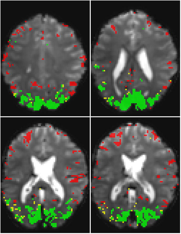
The various masks used for the analysis with correlation threshold 0.5 and 120 s worth of reference data, shown for 4 out of 10 slices for volunteer 2 (the same volunteer used for Figure 2). The area found to be significantly activated when analysis was performed without the noise-estimate regressor is shown in green. The additional voxels that were only significantly activated when applying the method described here are shown in yellow. All reference mask voxels are shown in red.

Figure 3 further shows that the voxels that form the correction mask R_Ref, derived using correlation analysis, are not randomly distributed over the brain. It can be seen that virtually all R_Ref-voxels are located in the grey matter, and that a substantial part of the R_Ref-voxels are clustered (e.g. in the posterior singulate area in the top-left panel, and the ventral-lateral area and middle-temporal cortex in the bottom-left panel of Figure 3).

DISCUSSION

In this work a method is presented that substantially increases the performance of fMRI experiments. It does not require any hardware or experimental changes, apart from the need to acquire a small amount of reference data. Based on the experimental findings described here, on the order of 1–2 minutes worth of reference data will probably be sufficient for robust performance under commonly used fMRI experimental conditions. In the experiments performed here there, results were not significantly different for reference data sets ranging from 30–270 s in length. The method results in the loss of a single degree of freedom during statistical analysis. Reducing the number of degrees of freedom will affect the noise distribution and therefore reduce the t-score. However, this penalty is typically low if the number of samples is sufficiently large. For example, for a p-threshold of 0.05 the loss for a reduction of one degree of freedom will be less than 1 % if there are more than 85 degrees of freedom remaining. The subset of data used for functional analysis in these experiments consisted of 300 time points, making this penalty negligible. Out of the 8540 voxels (over 5 volunteers) in this experiment that were significantly activated when the correlated noise regressor was not used in analysis, t-score decreased in 1146 voxels (13.4 %) when using a design matrix that does contain the correlated noise regressor. The average t-score decrease in those 1146 voxels was 0.6 %. In the remaining 86.6 % of the voxels, the t-score increased on average 12.0 % when accounting for correlated noise. The overall average t-score change was 10.3 %. Note that this average over all voxels is not identical to the 11.3 % reported in Table 1, since the value in Table 1 is the average over volunteers.

Since the same p-threshold was used to determine which voxels are considered significantly activated, the false-positive rate should not be affected by application of this method, assuming that the residual noise is normally distributed, which may not be the case due to the physiological noise contribution. Temporal autocorrelation correction should compensate for some of this effect. However the true false-positive rate, or the effect of the proposed method thereon, cannot be easily assessed. Since additional noise is accounted for by the proposed method, the false-negative rate is presumably reduced, resulting in an increase of the number of activated voxels.

One could argue that the time used for the acquisition of reference data could have been used to acquire additional fMRI data, which would also increase t-score. However, the performance increase obtained with the method proposed here was larger than can be expected based on additional sampling. For example, analysis with 30 s worth of reference data yielded a t-score increase of 11.0±2.5 %, whereas a t-score increase of 4.9 % could be expected if a similar 30-s longer fMRI experiment was performed, if all noise is assumed to be random. The benefit will further increase if the same reference data are used in the analysis of several datasets.

Furthermore, the exclusion of voxels in the reference region (R_Ref) could be seen as a disadvantage of the proposed method. However, the voxels in R_Ref were not deemed significantly activated in the analysis that does not account for correlated noise. Therefore, the exclusion of these voxels cannot be considered a drawback of this method, since all voxels that were significantly activated in the original analysis are inherently excluded from R_Ref, and therefore included in the final analysis. Subsequently, the exclusion of voxels in R_Ref cannot lead to a reduction of the number of activated voxels.

The data in Table 1 suggest an apparent discrepancy. The observed variance decrease is not in agreement with the increase in t-score found for the same volunteer. This is the result of two effects. First, the t-score scales with the inverse of the standard deviation. Therefore, averaging changes in variance (the square of SD) does not correspond to the resulting average in t-score. Second, the IDL code used for analysis detected and corrected serial correlation in the regression analysis. Since the correction only accounted for correlation between neighboring time points, it affected some regressors more than others, depending on their frequency characteristics. As a result, the overall decrease in variance was smaller than the decrease in the estimated variance of the amplitude of the block paradigm regressor. In order to demonstrate that this was the origin of the discrepancy, the analysis was performed a second time without performing the serial correlation correction (data not shown). When the serial correlation correction step was skipped, the changes in t-score exactly matched the changes in signal stability (1/SD). In addition, the observed changes in fitted activation amplitude dropped below 0.0001 %, demonstrating that the small changes in fitted amplitude in our data were the result of this correction as well.

For the data in this paper, a correlation threshold of 0.5 was used for the selection of the reference-region voxels. Choice of this threshold was somewhat arbitrary. Increasing the threshold will lead to a decrease of the number of voxels included in the mask. If the number of voxels in the correlation mask is small, thermal noise will potentially not be sufficiently averaged out when the regressor is computed. On the other hand, lowering the threshold too much could lead to the inclusion of too many noisy voxels in the regressor, as well as cause more voxels to be excluded from the final processing step. Sensitivity for threshold changes was low however, as can be seen in Table 1.

In the proposed method, the correlated noise regressor is orthogonalized with respect to the other regressors in the design matrix, most notably the activation paradigm regressor. This assures the removal of any residual activation signal from the correlated noise regressor, thereby assuring that all activation is fitted by the paradigm regressor and not erroneously assigned to the correlated noise regressor. A drawback of this approach is that the (generally small) bias resulting from a possible correlation between the paradigm and correlated noise is not removed. This bias is not introduced by or exacerbated by the proposed method. The exact same bias also affects the conventional analysis that does not account for correlated noise. This bias could potentially be removed by using non-orthogonalized regressors. However, apart from the reduced accuracy of the coefficients computed using regression analysis with a non-orthogonal design matrix, it is in practice difficult to obtain a proper estimate of the correlated noise that does not contain residual activation. The reference region (R_ref) can contain a limited amount of activation (below the detection threshold), which will contribute to the correlation between the correlated noise regressor and the paradigm regressor. This true activation (signal changes over time that are the result of the task) cannot be separated from actual correlated noise (other signal changes over time that happen to partially coincide with, but are unrelated to, the task) that has some degree of correlation with the paradigm.

Employing non-orthogonalized regressors with the proposed method is straightforward. When repeating the analysis using such a modified approach, a mean t-score increase of 9.5±2.7 % (compared to 11.3±1.6 % for the fully orthogonalized design matrix, see Table 1) was found, as well as a BOLD amplitude change of −1.38±1.7 % (compared to −0.11±0.1 for the orthogonalized design matrix). The variance change was identical for the two approaches, as is to be expected, since the same signals can be described by both design matrices, albeit with different coefficients for the paradigm- and correlated noise regressors.

While preparing this manuscript, we became aware of recent work by Fox et al. (13), in which spontaneous signal fluctuations in the left somatomotor cortex (LMC) were found to be correlated to the fluctuations in the right somatomotor cortex (RMC). Subtraction of the average RMC signal was used to improve the signal in LMC. Although this work shows similarities to the method presented here there are also some important differences. First of all, the coherent noise descriptor is derived from the equivalent anatomical area in the opposing hemisphere, whereas our method is generalized by using correlated voxels from the entire brain. A separate step is used to subtract the RMC signal from LMC, and the noise-descriptor is not decorrelated from other functional regressors in the subsequent functional analysis. This can negatively affect performance (9), here it lead to loss in activation amplitude in LMC of 11% on average over 11 subjects.

The source of the fluctuations removed by the method presented here was not further investigated. Possible sources are the cardiac- and/or respiratory cycle, as well as activity in cortical networks that are unrelated to the stimulus paradigm (often referred to as resting state fluctuations (19,20)). Although artifacts related to the cardiac- and respiratory fluctuations can be adequately removed using other methods (e.g. RETROICOR (8)), such methods typically require the acquisition of independent physiological data (for example using respiratory bellows and a pulse oximeter), and lead to a greater reduction of the number of degrees of freedom than the method presented here. Since the spatial extent of these possible contributors to the correlated noise regressor applied here is unlikely to change during the time span of a typical exam, the acquisition of a single reference scan is expected to be sufficient, although this has not been investigated.

In conclusion, this method allows for substantial increases of fMRI paradigm detection sensitivity at the cost of the loss of a single degree of freedom (which is accounted for in our functional analysis) and the need for the acquisition of a limited amount of additional data (on the order of one minute per volunteer per session for the scan parameters used here). The method was demonstrated here using block paradigm data, but can be used to correct any kind of over-determined fMRI experiment, including single-event and event-related fMRI experiments.

References

- 1.Ogawa S, Lee TM, Nayak AS, Glynn P. Oxygenation-sensitive contrast in magnetic resonance image of rodent brain at high magnetic fields. Magn Reson Med. 1990;14(1):68–78. doi: 10.1002/mrm.1910140108. [DOI] [PubMed] [Google Scholar]
- 2.Bartha R, Michaeli S, Merkle H, Adriany G, Andersen P, Chen W, Ugurbil K, Garwood M. In vivo 1H2O T2+ measurement in the human occipital lobe at 4T and 7T by Carr-Purcell MRI: detection of microscopic susceptibility contrast. Magn Reson Med. 2002;47(4):742–750. doi: 10.1002/mrm.10112. [DOI] [PubMed] [Google Scholar]
- 3.de Zwart JA, Ledden PJ, van Gelderen P, Bodurka J, Chu R, Duyn JH. Signal-to-noise ratio and parallel imaging performance of a 16-channel receive-only brain coil array at 3. 0 Tesla. Magn Reson Med. 2004;51(1):22–26. doi: 10.1002/mrm.10678. [DOI] [PubMed] [Google Scholar]
- 4.Weisskoff RM. Simple measurement of scanner stability for functional NMR imaging of activation in the brain. Magn Reson Med. 1996;36(4):643–645. doi: 10.1002/mrm.1910360422. [DOI] [PubMed] [Google Scholar]
- 5.Heim S, Amunts K, Mohlberg H, Wilms M, Friederici AD. Head motion during overt language production in functional magnetic resonance imaging. Neuroreport. 2006;17(6):579–582. doi: 10.1097/00001756-200604240-00005. [DOI] [PubMed] [Google Scholar]
- 6.Thévenaz P, Ruttiman UE, Unser M. Iterative multi-scale registration without landmarks. IEEE international conference on image processing; Washington, DC, USA. 1995. pp. 228–231. [Google Scholar]
- 7.Lee CC, Jack CR, Jr, Grimm RC, Rossman PJ, Felmlee JP, Ehman RL, Riederer SJ. Real-time adaptive motion correction in functional MRI. Magn Reson Med. 1996;36(3):436–444. doi: 10.1002/mrm.1910360316. [DOI] [PubMed] [Google Scholar]
- 8.Glover GH, Li TQ, Ress D. Image-based method for retrospective correction of physiological motion effects in fMRI: RETROICOR. Magn Reson Med. 2000;44(1):162–167. doi: 10.1002/1522-2594(200007)44:1<162::aid-mrm23>3.0.co;2-e. [DOI] [PubMed] [Google Scholar]
- 9.Deckers RH, van Gelderen P, Ries M, Barret O, Duyn JH, Ikonomidou VN, Fukunaga M, Glover GH, de Zwart JA. An adaptive filter for suppression of cardiac and respiratory noise in MRI time series data. Neuroimage. 2006;33(4):1072–1081. doi: 10.1016/j.neuroimage.2006.08.006. [DOI] [PMC free article] [PubMed] [Google Scholar]
- 10.Wise RG, Ide K, Poulin MJ, Tracey I. Resting fluctuations in arterial carbon dioxide induce significant low frequency variations in BOLD signal. Neuroimage. 2004;21(4):1652–1664. doi: 10.1016/j.neuroimage.2003.11.025. [DOI] [PubMed] [Google Scholar]
- 11.Friston KJ, Frith CD, Liddle PF, Frackowiak RS. Functional connectivity: the principal-component analysis of large (PET) data sets. J Cereb Blood Flow Metab. 1993;13(1):5–14. doi: 10.1038/jcbfm.1993.4. [DOI] [PubMed] [Google Scholar]
- 12.Bell AJ, Sejnowski TJ. An information-maximization approach to blind separation and blind deconvolution. Neural Comput. 1995;7(6):1129–1159. doi: 10.1162/neco.1995.7.6.1129. [DOI] [PubMed] [Google Scholar]
- 13.Fox MD, Snyder AZ, Zacks JM, Raichle ME. Coherent spontaneous activity accounts for trial-to-trial variability in human evoked brain responses. Nat Neurosci. 2006;9(1):23–25. doi: 10.1038/nn1616. [DOI] [PubMed] [Google Scholar]
- 14.de Zwart JA, van Gelderen P, Kellman P, Duyn JH. Application of sensitivity-encoded echo-planar imaging for blood oxygen level-dependent functional brain imaging. Magn Reson Med. 2002;48(6):1011–1020. doi: 10.1002/mrm.10303. [DOI] [PubMed] [Google Scholar]
- 15.Waldvogel D, van Gelderen P, Muellbacher W, Ziemann U, Immisch I, Hallett M. The relative metabolic demand of inhibition and excitation. Nature. 2000;406(6799):995–998. doi: 10.1038/35023171. [DOI] [PubMed] [Google Scholar]
- 16.Durbin J, Watson GS. Testing for serial correlation in least squares regression. III Biometrika. 1971;58(1):1–19. [PubMed] [Google Scholar]
- 17.Watson GS. Serial correlation in regression analysis. I Biometrika. 1955;42:327–341. [Google Scholar]
- 18.Woolrich MW, Ripley BD, Brady M, Smith SM. Temporal autocorrelation in univariate linear modeling of FMRI data. Neuroimage. 2001;14(6):1370–1386. doi: 10.1006/nimg.2001.0931. [DOI] [PubMed] [Google Scholar]
- 19.Biswal B, Yetkin FZ, Haughton VM, Hyde JS. Functional connectivity in the motor cortex of resting human brain using echo-planar MRI. Magn Reson Med. 1995;34(4):537–541. doi: 10.1002/mrm.1910340409. [DOI] [PubMed] [Google Scholar]
- 20.Raichle ME, MacLeod AM, Snyder AZ, Powers WJ, Gusnard DA, Shulman GL. A default mode of brain function. Proc Natl Acad Sci U S A. 2001;98(2):676–682. doi: 10.1073/pnas.98.2.676. [DOI] [PMC free article] [PubMed] [Google Scholar]