Abstract
Objective
The objective of the proposed research is to develop a methodology for modeling and evaluation of human motions, which will potentially benefit patients undertaking a physical rehabilitation therapy (e.g., following a stroke or due to other medical conditions). The ultimate aim is to allow patients to perform home-based rehabilitation exercises using a sensory system for capturing the motions, where an algorithm will retrieve the trajectories of a patient’s exercises, will perform data analysis by comparing the performed motions to a reference model of prescribed motions, and will send the analysis results to the patient’s physician with recommendations for improvement.
Methods
The modeling approach employs an artificial neural network, consisting of layers of recurrent neuron units and layers of neuron units for estimating a mixture density function over the spatio-temporal dependencies within the human motion sequences. Input data are sequences of motions related to a prescribed exercise by a physiotherapist to a patient, and recorded with a motion capture system. An autoencoder subnet is employed for reducing the dimensionality of captured sequences of human motions, complemented with a mixture density subnet for probabilistic modeling of the motion data using a mixture of Gaussian distributions.
Results
The proposed neural network architecture produced a model for sets of human motions represented with a mixture of Gaussian density functions. The mean log-likelihood of observed sequences was employed as a performance metric in evaluating the consistency of a subject’s performance relative to the reference dataset of motions. A publically available dataset of human motions captured with Microsoft Kinect was used for validation of the proposed method.
Conclusion
The article presents a novel approach for modeling and evaluation of human motions with a potential application in home-based physical therapy and rehabilitation. The described approach employs the recent progress in the field of machine learning and neural networks in developing a parametric model of human motions, by exploiting the representational power of these algorithms to encode nonlinear input-output dependencies over long temporal horizons.
Keywords: Physical rehabilitation, Mathematical model, Neural networks, Auto-encoder, Mixture density network, Performance metric, Recurrent neural networks, Time series
Introduction
Mathematical modeling of human motions is a research topic in several scientific fields, and subsequently it has been employed across a wide range of applications. Nevertheless, from a general point of view modeling of human motions remains a challenging problem, due to several aspects related to their intrinsic properties. First, human movements are inherently random, as a consequence of the stochastic nature of processing of the motory commands by the brain [1] (e.g. we cannot re-create identical movements or draw perfectly straight lines). Second, human motions have a highly nonlinear character, as all other processes in the nature. And third, the complex levels of hierarchy in the human reasoning are also reflected in the way the brain controls the limbs in executing desired motions.
The proposed research aims to exploit the recent progress in the field of deep artificial neural networks (NN) for modeling of human motions. The motivation stems from the demonstrated potential of deep NN architectures to encapsulate highly nonlinear relations among sets of observed and latent variables, as well as the capacity to encode data features at multiple hierarchical levels of abstraction. These properties have been conducive to the development of efficient deep NN algorithms that in recent times outperformed other machine learning methods in a number of international competitions and applications [2,3]. However, this success has been largely based on the use of convolutional NN that have proven suitable for dealing with spatial data, such as pixels in static images. On the other hand, human motion data possess quite a different structure due to the strong temporal correlation among the data points, and require different type of NN architectures. One such architecture designed for dealing with sequential data is the recurrent NN (RNN) [4]. More specifically, RNNs introduce recurrent connections between the neuronal activations of the neighboring units in sequences. The recurrence property establishes a basis for extracting the underlying temporal dependencies in sequential data. Unlike the current approaches for human motion modeling, such as Gaussian process model [5], hidden Markov models [6], dynamic movement primitives [7] or Kalman filters [8], which are based on short-term primarily linear approximation of the motion dynamics, recurrent NNs offer representational power for encoding non-linear motion dynamics over longer temporal horizons.
The proposed work employs RNNs for developing a mathematical model of human motions, by extracting latent states of the motion sequences, related to sub-goals in executing the motion. To tackle the stochastic character of human movements, we propose a statistical modeling approach, based on the provision of multiple examples of a motion performed under similar conditions. The model aims to probabilistically encode the performed motion with a mixture of Gaussian probability density functions, by exploiting the variability across the motion examples. The network architecture consists of an autoencoder subnet [9] of LSTM neurons for dimensionality reduction of the observed motion data, and a mixture density network (MDN) [10] for modeling the conditional density function of the spatial coordinates, conditioned on the temporal coordinates of the motion. The obtained probabilistic model of the human motions is afterwards used for evaluation of newly observed motion sequences.
Related Work
Physical rehabilitation
Physical rehabilitation therapy is crucial for patients recovering from stroke, surgery, or musculoskeletal trauma. A study published by Machlin et al. [11] analyzed the Medical Expenditure Panel Survey generated by the US federal government, and indicated that in 2007 the cost of physical rehabilitation therapy in US was approximately $13.5 billion. These expenditures were incurred during approximately 88 million physical therapy episodes by nearly 9 million adults.
The physiotherapist supervised treatments represent only a fraction of the total rehabilitation treatment; over 90% of the exercises are performed by patients in a home-based setting, also known as home exercise programs [12]. In this case, a physiotherapist instructs a patient on the type of physical exercises to be performed, and the patient is expected to perform the exercises, and continuously record their progress in a logbook. The patient will periodically attend follow-up visits with the physiotherapist, who evaluates their progress, and may prescribe a new set of exercises. However, there is a multitude of reports in the literature of low adherence rates to prescribed exercises in home-based rehabilitation, ranging between 11% and 40% [13,14]. The poor compliance delays functional recovery, prolongs the rehabilitation period, and increases healthcare cost.
Among the key factors contributing to low adherence to physiotherapy in outpatient environment is the lack of supervision, evaluation, and motivation for continued treatment [15]. Accordingly, the need for tools that support home-based rehabilitation has been widely recognized. The recent emergence of low cost non-intrusive motion capture sensors, such as Microsoft’s Kinect, stimulated a wave of research and proliferation of applications in this domain [16,17]. KiReS (Kinect Rehabilitation System) [18] and VERA (Virtual Exercise Rehabilitation Assistant) [12] are examples of systems that employ a Kinect sensor for tracking a patient’s movements, and provide a graphical interface with avatars showing the desired exercise as prescribed by the physiotherapist and the current motions of the patient. Such visualization tools are conducive toward improved adherence to the prescribed physical therapy by allowing review of the exercises by the patients and correcting the performance, as well as by providing a means for remote review of the patient’s progress by the physiotherapist.
A key prerequisite for monitoring and evaluation of patients’ progress in home exercise programs is the provision of efficient and comprehensive performance evaluation metrics. The existing clinical evaluation metrics, such as Fugl-Meyer assessment (FMA), Wolf motor function test (WMFT), and the ratio of optimal versus sub-optimal motion execution [12,18], were primarily designed for assessment performed by a physiotherapist. The development of performance evaluation metrics based on sensor captured motions in outpatient setting remains an open research topic.
We hold that formalization of efficient evaluation metrics is predicated on congruent mathematical models for representation of human motions. In this work, we propose an approach for probabilistic modeling and evaluation of human motions based on the latest advances in artificial neural networks.
NN for motion modeling
The approaches for human motion modeling and representation are broadly classified into two categories: a group that uses latent states for describing the temporal dynamics of the movements, and another category that employs local features for representing the motion. Among the methods based on introduced latent states, the most prominent are Kalman filters, hidden Markov models [19], and Gaussian mixture models [20]. Main shortcomings of these methods originate from employing linear models for the transitions among the latent states (as in Kalman filters), or from adopted simple internal structure of the latent states (typical for hidden Markov models). On the other hand, the approaches based on extracting local features within the motion data, e.g. key points [21], and temporal pyramids [22], are typically based on predefined criteria for feature representation which are often task-specific and defined at a single level of task abstraction. These attributes limit the ability of the feature class of motion representation methods to handle arbitrary spatio-temporal variations across the motion sequences in an efficient manner.
The recent development in the field of artificial NNs stirred a significant interest in their application for modeling of human motions as well. The capacity for motion classification without the need for segmentation has been employed in several works. For example, Baccouche et al. [23] employed a convolutional NN for feature extraction fused with a layer of recurrent units for action recognition, and Lefebre et al. [24] implemented bidirectional RNN for gesture classification.
Further, the replacement of simple RNN units with LSTM units mitigated the problem of vanishing/exploding gradients and provided a base for training deep RNNs. Subsequently, a body of work emerged that implemented deep NN for modeling of human motions.
For examples, the approach by Du et al. [25] employs a deep RNN for hierarchical modeling of human motions, where input sequences consisting of skeletal joint positions of the human body are divided into five groups, related to the joints of the trunk and of the four body limbs. By fusing the input data of the five body groups progressively through the layers of neurons, the approach demonstrated high-performance in classification of human motions.
Another recent work [26] implements an encoder-decoder network with recurrent LSTM units for extracting salient features in human motion sequences. The resulting encoded representation is afterwards successfully utilized for both motion generation and for body parts labeling in videos.
In the work by Zhu et al. [27] the authors investigated the regularization in deep RNNs for human action recognition, and proposed 2 techniques for this purpose. One is based on learning co-occurrence features in the motion data across the layers of neurons, and another is a dropout technique applied on the gates within the LSTM units. The proposed regularization produces improved performance over the state-of-the-art methods.
Jain et al. [28] developed a novel NN architecture that introduces spatio-temporal graphs in its structure. More specifically, the factor components in the st-graphs are grouped and modeled with RNNs. The framework is evaluated for prediction and generation of human actions, and for understanding human-object interactions.
The above listed methods are employed for classification of human actions, or for predicting future motion patterns in a generative fashion, based on encoded joint distribution of the input data and the hidden states. The presented approach in this article employs RNNs for probabilistic modeling of human motions using density function estimation. To the best of our knowledge, such an implementation is novel and differs from the previous works on human motion modeling within the published literature. Several recent studies have successfully applied mixture density networks within an RNN framework to model complex datasets. For example, the work in [29] employed MDN and RNNs for classification and prediction of biological cell movement in different environments based on recorded motion sequences. Similar works reported application of MDN in modeling visual attention [30], wind speed forecasting [31], and acoustic speech modeling [32].
Problem Formulation
The problem is related to a rehabilitation exercise prescribed by a physiotherapist to a patient by demonstrating the required motion in front of the patient. The demonstration can be either performed by the physiotherapist, or by moving patient’s limbs. It is assumed that the physiotherapist will demonstrate the motion multiple times (typically between 5 and 10 times), for the patient to understand the underlying range of movement of the different body parts. The patient is then asked to repeat the motion in a home-based rehabilitation environment a specified number of times in a daily session, or during multiple daily sessions. The goal of our research is to develop an algorithm for modeling the demonstrated motion and for evaluation of the performance of the patient during home rehabilitation in order to conclude whether the performed motions by the patient correspond to the prescribed motions by the physiotherapist.
In practice, the physiotherapist may demonstrate the motion only once or twice; since our brains are excellent at pattern recognition, and we can easily generalize from only a single example of a task. On the other hand, machine learning algorithms are data driven and require multiple examples of a task to accurately extract underlying patterns in the data. Furthermore, the physiotherapist in reality will support the demonstrations by verbal explanations of the movements, and he/she can also demonstrate several incorrect examples of performing the motion. In the considered study, verbal explanations and non-optimal demonstrations are ignored, and the focus is on motion learning from perceived sensory data. The above scenarios can be considered as avenues for future work.
It is assumed that a sensory system is available for capturing the demonstrated motion as prescribed by the physiotherapist. The number of demonstrated examples of the motion is denoted M, and the measurement by the sensory system for each of the demonstrated examples of the motion is denoted Om, where m is used for indexing the individual demonstrated examples. The set of observed demonstrations comprises . Also each perceived motion example Om is a temporal sequence of high-dimensional sensory data, and it is denoted , where represents the sensory measurement at time, t1 i.e., the superscripts are employed for indexing the temporal position of the measurements within each motion sequence, and Tm denotes the number of measurements in each observed sequence. In general, the demonstrated examples will have different lengths, i.e., different number of measurements Tm. Each individual measurement is a D-dimensional vector, hence the notation adopted is , where k is the current time step. The above notation employs bold font type for representing vectors and matrices.
For example, let’s consider a motion that is demonstrated 7 times by the physiotherapist. In that case, the set of demonstrated examples of the motion is . Each motion is a time series representing a sequence of measurements by the sensory system. For instance, if an optical tracker collected the measurements at a rate of 100 measurements per second, and if the duration of the third motions was 4.2 seconds, then the sequence O3 will consist of 420 measurements, and it will be represented as , with t1=0.01s, t2=0.02s and t420=4.2s. Furthermore, if the sensory system used 10 optical sensors for capturing the motions, and the outputs are 3-dimensional spatial coordinates of the optical sensors, each individual measurement will represent 30-dimensional data signal. In that case, the measurement of the third motion example at time step 2 will be the 30-dimensional vector .
Next, it is assumed that the same sensory system for motion perception is used to capture the motions of the patient during the rehabilitation exercises. Let’s denote the observation of the patient’s performed motion with R. Similar to the above notation, the motion sequence R will consist of TR D-dimensional measurements r(k), i.e., .
The patient will attempt to reproduce the motion as demonstrated by the physiotherapist. Due to pain or other conditions, the patient may not be able to achieve the range of the motion as requested, or he/she may perform the motion in a wrong way due to a variety of reasons. The objective of the presented research is to evaluate the performance of the patient with regards to the physiotherapist demonstrated examples of the motion. Or, in other words, the objective is to evaluate how consistent patient’s motion R is with the reference motion set .
The problem was approached on the grounds of the fact that human motions are intrinsically stochastic. We cannot reproduce a motion in identical manner, due to the stochastic character of the motor actions as directed by the neural networks in the human brain. The variance within the human movements can be exploited to probabilistically model the motions. Using the observed set of examples of the motion provided by the physiotherapist O, a probabilistic model of the motion will be derived described with a set of parameters λ. The parameters will be estimated by maximizing the probability of the observed data, argOmax P (λ|O). The probabilistic model will then be used for estimating the probability that the patient’s motion belongs to the distribution parametrically defined with λ, i.e., P (R|O).
The considered problem is an unsupervised learning problem, where the goal is to develop a probabilistic model of the observed data by determining the density estimation within a projected space with reduced dimensionality. The obtained model will be used to probabilistically evaluate new observations.
Network Architecture
The proposed network architecture is shown in Figure 1. Input to the network is a sequence of vectors related to the sensory perception of the motion O. A recurrent layer of LSTM units encodes input sequences Om into low-dimensional sequences Zm. The sequences Zm are decoded by another recurrent layer of LSTM units to the input context Om. The obtained low-dimensional sequences Zm are processed through another recurrent layer of neuron units, and the resulting sequences Ym are probabilistically encapsulated by a mixture of Gaussian probability distributions, parameterized with a set of means μ, standard deviations σ, and mixing coefficients π. The theoretical background behind the network architecture is presented next.
Figure 1.
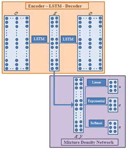
The proposed network architecture, where the arrows denote the flow of data in the network.
Recurrent neural networks
RNNs [4] are a subclass of neural networks that introduce recurrent connections between the neuron units. This type of NN has been designed for processing sequential data, such as time series, textual data, or DNA protein sequences. The recurrent connections between the neuron units enable capturing sequential (or temporal) dependencies across the input data (Figure 1).
For an input sequence with length Tm consisting of an array of vectors , where k denotes the position of the vector within the sequence Om, RNNs introduce a sequence of hidden states that establish a mapping between the input and output data of the network. In temporally ordered sequences k would correspond to the time index tk of the input values. An RNN is graphically represented in Figure 2. The network structure is shown at the sequence level in Figure 2(a), as well as unfolded along the time steps 1,2,….,k−1, k, k+1,.. in Figure 2(b). The connections between the consecutive neuron units h(k), represented with the colored nodes in the Figure 2, enable information about the input data to be shared with the neighboring neuron units. The recurrence furnishes the network with a memory capability, i.e., past observations can be employed for understanding the current observation, or for predicting future observations in a sequence.
Figure 2.

Graphical representation of an RNN. (a) A sequence of input data Om is connected to a sequence of hidden units H with recurrent connections between the hidden units. (b) The unfolded sequence Om consists of observation vectors represented with white nodes, and the sequence H consists of hidden state vectors h(k) represented with colored nodes.
The outputs of the hidden unit vectors h(k) in the RNN network presented in Figure 2 are calculated as,
| (1) |
where Woh denotes the matrix of connection weights from the input vectors to the hidden layer units h(k), Whh denotes the matrix of recurrent connection weights between the hidden layer units, bh denotes the vector of bias values, and f is an activation function. The hidden layer H will further be connected to an output sequence, or to another hidden layer in the network structure. The weight and bias parameters in RNNs are learned with the back-propagation through time (BPTT) algorithm [33], by minimizing a loss function over the set of training sequences .
Two significant shortcomings of conventional RNNs presented in equation (1), are the inability to capture long-term dependencies in the data, and the problem of vanishing/exploding gradients in learning the network parameters [34]. These are overcome by introducing special forms of recurrent neuron units, among which the most common are the LSTM units, which stands for long short-term memory [35]. A graphical representation of an LSTM unit is given in Figure 3. The information processing in LSTM is characterized with the use of several gates which control the amount of information that is passing through the hidden units. Hence, each LSTM unit has an input gate, forget gate, and output gate. The gates are used for controlling the internal state of the LSTM unit stored in a memory cell. The memory cell accumulates information and carries it from the past to the future temporal states in the layer, thus enabling establishment of long term dependencies across the data sequence.
Figure 3.
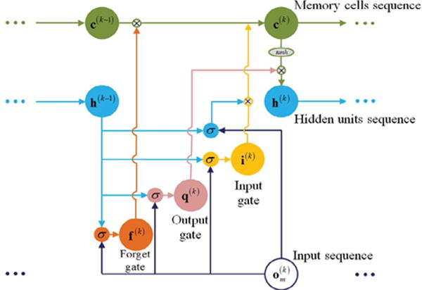
Graphical representation of the data flow within an LSTM unit.
Computations within the kth LSTM unit are as follows:
| (2) |
| (3) |
| (4) |
| (5) |
| (6) |
where W’s denote the matrices of weight values, b’s denote the vectors of bias values, and σ and tanh denote a sigmoid and hyperbolic tangent functions, respectively. Similar to Figure 2, the notation and h(k) is related to the observed input vector and the output vector from the layer of hidden units at time tk, whereas i(k), f(k), q(k), and c(k) denote the corresponding activations of the input gate, forget gate, output gate, and the memory cell, respectively.
At each time step k, the forget gate regulates the amount of the information in the memory cell that is discarded, the input gate determines how much new information to store in the memory cell and pass it to the next units, and the output gate controls the fraction of the information in the memory cell to be output by the hidden unit. Furnished with the ability to retain and selectively pass information through the gates of an LSTM unit, the network can learn long-term temporal correlations within the data sequences (Figure 3).
Autoencoder neural networks
Autoencoders refer to an NN architecture designed to learn a different representation of a set of input data, through a process of data reconstruction [9,36]. The intent is to extract useful attributes within the data, achieved by setting the network output to be equal to the original input. The step of transforming the input data to a different representation is called encoding, and analogously, the operation of reconstructing the data from its approximation is called decoding.
A graphical representation of an autoencoder network is depicted in Figure 4. As shown in the figure, the network consists of an encoder portion which maps the input data into a code representation , and a decoder portion which reprojects the code Ζ into the input O. If the mapping function of the encoder is denoted φ: O→ Ζ, and the moping function of the approximation by the decoder is denoted ψ: Ζ→ Ô, the connection weights in the autoencoder network are learned by minimizing the reconstruction error formalized as :
Figure 4.
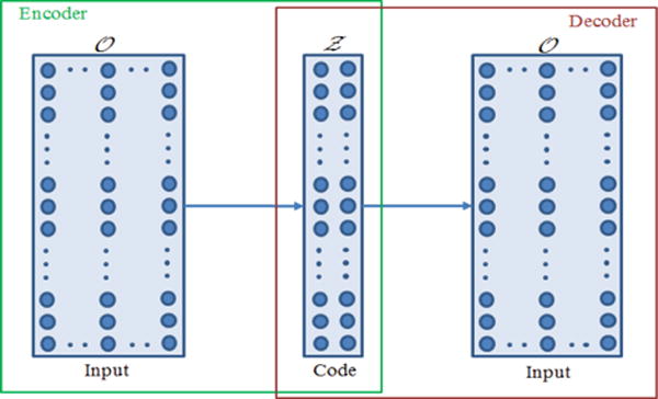
Graphical representation of an autoencoder NN.
The majority of autoencoders employ a code representation with lower dimensionality in comparison to the input data. This forces the network to learn a sparse representation of the input data, and with that to extract the most salient attributes within the data to produce minimal reconstruction error. Due to these properties, typical application tasks of autoencoder NNs are dimensionality reduction, feature extraction, and data denoising.
In this study on modeling of human motions, an autoencoder is employed to reduce the dimensionality of the observed sequences, since the dimensionality of the data in motion capture systems is typically in the range of 40 to 60 measurements per time step. On the other hand, not all of the body parts are usually involved in performing a motion, and in addition, the movements of the individual body parts are highly correlated. Hence, projection of the measurement data to a lower dimensional space is helpful in extracting high-level features within the human motions, and facilitates the tasks of modeling and analysis of the motions.
Regarding the dimensionality reduction using autoencoders, if the connection weights between the input and the hidden layers are linear, and mean squared error is used as a loss function, the network learns the principal components of the input data, and in this sense it operates as a PCA (principal component analysis) processor. The provision of nonlinear functions for neuron activations in autoencoders allows extracting richer data representations for dimensionality reduction. Furthermore, by stacking several consecutive encoding and decoding layers of hidden neurons, deep autoencoder networks are created, which can additionally increase the representational power capacity (Figure 4).
Mixture density networks
MDNs are a network architecture that employs a mixture of probability density functions in modeling dependencies in the input data [10]. Let’s assume input sequences and with length Tm consisting of d-dimensional vectors and , respectively, which in general do not have to be ordered sequences. MDNs estimate the conditional probability density function for k=1,2,…,Tm, as a mixture of probability distributions.
If Gaussian probability distributions are adopted as the mixture components, then the conditional probability density function is expressed as
| (7) |
In the equation, L is the number of Gaussian mixture components, πl denote the vector of mixing coefficient of the Gaussian component l, and N(y|μ,σ2) denotes a multivariate Gaussian probability distribution with a mean μ and variance σ2. Note in equation (7) that the mixture parameters are dependent on the input vectors .
The parameters in MDNs are estimated by minimizing a loss function defined by the negative log-likelihood of the input and output data.
| (8) |
With regards to the requirement for the mixing coefficients πl ≥ 0 and , the connections in MDN leading to the mixing coefficients are defined as soft max functions of the corresponding network output activations al,m, i.e.,
| (9) |
For the standard deviations, the requirement is satisfied by employing exponential functions of the network activations as follow
| (10) |
Lastly, the means are connected directly to the network activation by a linear projection layer
| (11) |
The output parameters of the network can be used for estimating the conditional average of a data sequence Yn given a sequence Xn as
| (12) |
as well as the expected variance of the conditional density function as
| (13) |
Experiments
Motion perception
The work assumes that a Microsoft Kinect sensor will be used for capturing the motions for rehabilitation exercises. With a price tag of around $150, its use for home-based rehabilitation is much more feasible, when compared to the optical trackers or other similar motion capture systems that cost tens of thousands of dollars. The Kinect sensor includes a color camera and an infrared camera for acquiring image (RBG) and range data simultaneously. The software development kit (SDK) for Kinect by Microsoft provides libraries for access to the raw RGB and depth streams, skeletal tracking, noise suppression, etc. The capability for skeletal tracking has been widely used for capturing human motions. The skeleton consists of 20 points corresponding to the joints in the human body. During the skeleton tracking, the 3-dimensional position for each of the 20 joints is output at a rate of 30 frames per second.
Dataset
For proof of concept we used the publicly available dataset of human motions UTD-MHAD (University of Texas at Dallas-Multimodal Human Action Dataset) [37].
The UTD-MHAD dataset consists of 27 actions performed 4 times by 8 subjects. The data are collected with a Kinect sensor and a wearable inertial sensor, and is available in 4 different formats: RBG video, depth sequences, skeleton joint positions, and inertial sensor signals. Sample image for three of the actions: wave, bowling and draw circle, are shown in Figure 5.
Figure 5.
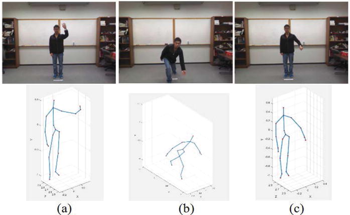
Sample images and skeletal representations for (a) Wave; (b) Bowling; and (c) Draw circle actions in the UTD-MHAD dataset.
Human motion modeling
The motion related to the swipe left action from the UTD-MHAD dataset is initially considered. The training set consists of 21 recorded sequences, performed 3 times by 7 of the subjects, i.e. O={O1,O2,…, O21} and the testing set consists of 7 sequences performed once by 7 of the subjects Q={Q1, Q1,…., Q7}, where the sets and are disjoint, i.e., O∩Q=∅. The length of the training sequences varied between 48 and 72 time frames. Each measurement includes the x, y, and z spatial positions of the 20 skeletal joints, i.e., the dimensionality of the vectors is D=60. In a preprocessing step the spatial joint positions were normalized to zero mean sequences, and to facilitate density estimation with a mixture of Gaussians, the sequences were temporally scaled and aligned to a constant length of 48 frames by using the dynamic temporal warping (DTW) algorithm [38].
The network architecture shown in Figure 1 is employed for processing the input data O. The code was implemented using the open-source Python libraries Theano [39] and Keras [40]. An autoencoder with recurrent layers of LSTM units is used for sequence-to-sequence processing. The code sequences are denoted Ζ={Ζ1,Ζ2,…,Ζ21}, as also shown in Figure 4. The encoder reduces the dimension of the input sequences Om equal to D=60 to dimension of the context Ζm equal to d=3. The autoencoder is trained in a mini-batch input mode to minimize the reconstruction error by using the AdaDelta gradient descent method [41] for updating the network parameters, whereas the gradients of the cost function are calculated with the BPTT algorithm [42].
The trained network is afterwards used for reconstructing the testing set of data. Examples of two testing sequences Qm, the corresponding encoded sequences , and the decoded sequences , for m∈{2,4}, are shown in Figure 6. One can note that the sequences for the swipe left action include only movement of the right hand of the subject, and most of the other body parts are almost stationary during the motion. Therefore, many of the 60-dimensional joint positions have values close to zero, and only several of the skeleton joints have varying position values during the motion. The encoded representation for the training sequences Ζ={Ζ1,Ζ2,…,Ζ21} is shown superimposed on Figure 7.
Figure 6.
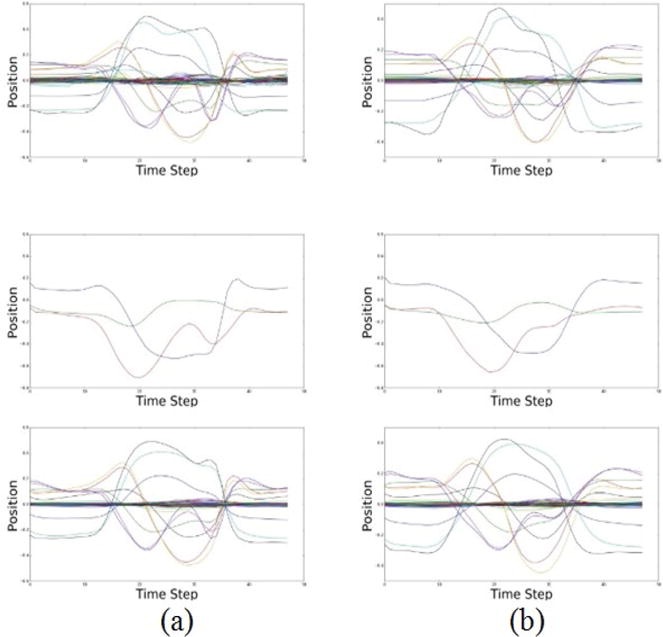
From top to bottom: (a) Testing sequence Q2, encoded representation , and reconstructed sequence ; (b) Testing sequence Q4, encoded representation , and reconstructed sequence
Figure 7.
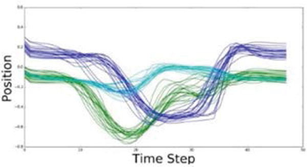
Encoded representation for all 21 training sequences.
The sequences are afterwards processed with an MDN network, depicted in Figure 1. As described in Section 5.3 the network is designed to learn mixture parameters encoding a conditional density function of the target data for given input data. The number or neurons in the layer connecting the output of the autoencoder network and the MDN output is set of 100. The layer has fully connected nodes to the set of sequences. Further, the number of Gaussian mixture components in the network is set to L=4. The independent component of the input Xm is related to the temporal ordering of the sequences, and the dependent component, or the target, Ym, is related to the spatial position of the Ζm sequences. More specifically, the inputs to the MDN comprise arrays of time steps Xm=(1,2,….,48) for all X sequences, and the targets are for all Y sequences, i.e., for m=1,2,….,21. The network estimates the parameters of Gaussian mixture components by maximizing the likelihood of the input data, which is commonly performed by minimizing the cumulative negative log-likelihood P(Ym|Xm) for m=1,2,….,21. Contours of the negative log-likelihood for the three dimensional position sequences are shown in Figure 8. The obtained mixture parameters are dependent on the input, that is, for each input value k a conditional probability distribution of the target is obtained given the value of the input k.
Figure 8.
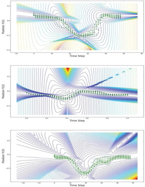
Contours of the conditional density functions for the three spatial coordinates of the target sequences, shown with green scattered markers.
The expected average and one standard deviation of the conditional density function for one of the target spatial dimensions is shown in Figure 9 for the case of 4 and 8 mixture components.
Figure 9.
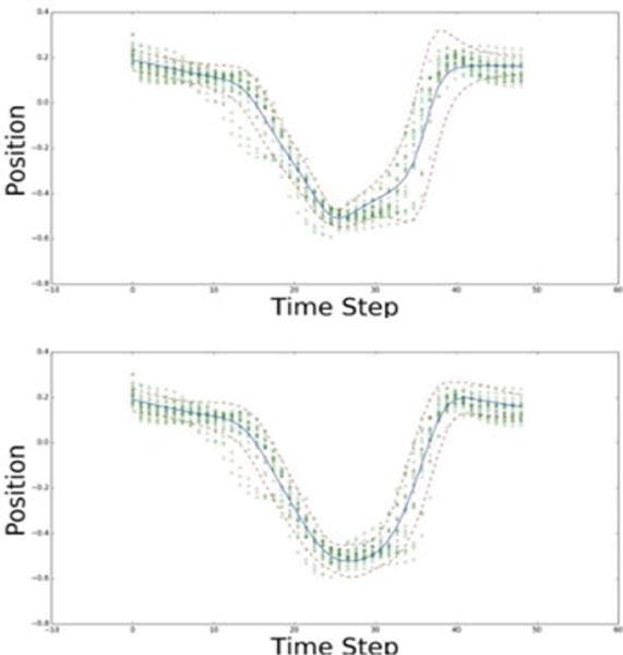
Expected average and one standard deviation of the density function for 4 mixture components (upper figure) and 8 mixture components (lower figure).
The Gaussian mixture parameters provide a probabilistic description of the average values and the underlying variability of the motion, as a function of its temporal evolution. The resulting parameterized density function is employed as a spatio-temporal model for evaluation of other motions.
Evaluation
Based on the learned model of a motion presented in the previous section, the next step is to evaluate a new motion sequence, presumably performed by a patient during a home-based rehabilitation therapy Figure 9. The sequence is denoted .
One possible metric for evaluation of the sequence R with regards to the probabilistic model described with the MDN parameters is the mean log-likelihood of the sequence given the model parameters LR=(R|λ), calculated as
| (14) |
where t(k) is the sequence of time step indices of the spatial positions of the sequence R.
The mean log-likelihood for the 21 training sequences is shown with the blue line in Figure 10. The mean log-likelihood was also calculated for observed sequences corresponding to other motions in the dataset, such as swipe right, waving, and clapping, and is shown with red lines in Figure 10. As expected, the sequences that are not produced by the swipe left motion are less probable to fit within the density probability function described with the parameters.
Figure 10.
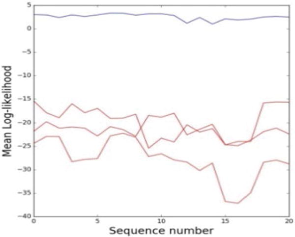
Mean log-likelihood for sequences from 4 different actions. The results related to the action swipe left used for training are shown with the blue line, and the results related to other actions are shown with the red lines.
Since the UTD-MHAD dataset does not provide examples of sub-optimal motions, such examples are synthetically generated here by adding random noise to the training data, for a proof of concept. Thus, several levels of uniformly distributed noise are added to the training sequences, and afterwards, the mean log-likelihood is evaluated. The result is presented in Figure 11. The levels of noise added are: 0.01, 0.1, 0.2, 0.4 and 1. The original sequences without added noise are shown with the blue line in the figure. As more noise is added to the motion sequences, the log-likelihood decreases. For the noise of 0.01 shown with the red line in the figure, the difference with the original sequence is very small, since that level of noise is similar to the measurement noise within the sensory data. As expected, the sequences with added noise deviate from the original sequences that were used to develop the motion model, and their likelihood to belong to the probability density function is smaller.
Figure 11.
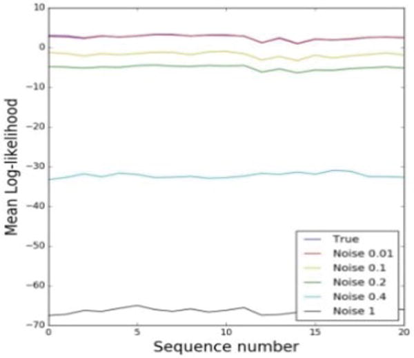
Mean log-likelihood for the swipe left action. The original sequences are shown with the blue line, and the sequences with added noise are shown with different line colors.
In a similar manner, motion sequences performed by a patient can be compared to a model of the motion as demonstrated by the physiotherapist. The mean log-likelihood can be used to assess the performance of the patient. As the patient continues with the rehabilitation therapy, the metric can be used to indicate whether there is a progress toward the prescribed motion. Figure 11. Mean log-likelihood for the swipe left action. The original sequences are shown with the blue line, and the sequences with added noise are shown with different line colors.
Summary
The article presents an approach for modeling and evaluating human motions using artificial neural networks. The network architecture consists of two subnets: an autoencoder and a mixture density subnet. The autoencoder employs layers of recurrent neuron units for dimensionality reduction and extraction of low-level features within the motion sequences, thus transforming noisy, high-dimensional datasets with strong correlations into a lower-dimensional dataset with low noise. The MDN portion of the network is used for density function representation of the motions with a mixture of Gaussian probability distributions. The output of the network is a probabilistic model of the human motions represented with a set of mixture parameters and a set of network connection weights.
The model is intended to be employed for evaluation of a patient performance in a home-based physical rehabilitation therapy. The probabilistic character of the proposed model allows employing statistical metrics for evaluation of patient’s performance. In this study, the probability, calculated as the mean log-likelihood of the motions performed by the patient, that the motions are drawn from the density function of the reference model, is adopted as a performance evaluation metric. For proof of concept, motion sequences from the available dataset have been distorted by adding random noise, and afterwards the mean log-likelihood is evaluated using the model parameters, and compared to the training set of motions.
Acknowledgments
This work was supported by the Center for Modeling Complex Interactions through NIH Award #P20GM104420 with additional support from the University of Idaho.
References
- 1.Clamann HP. Statistical analysis of motor unit firing patterns in a human skeletal muscle. Biophysics J. 1969;9:1223–1251. doi: 10.1016/S0006-3495(69)86448-9. [DOI] [PMC free article] [PubMed] [Google Scholar]
- 2.Schmidhuber J. Deep learning in neural networks: An overview. Neural Networks. 2014;61:85–117. doi: 10.1016/j.neunet.2014.09.003. [DOI] [PubMed] [Google Scholar]
- 3.Goodfellow I, Bengio Y, Courville A. Deep Learning. MIT Press; Cambridge, USA: 2016. [Google Scholar]
- 4.Rumelhart D, Hinton G, Williams R. Learning representations by back-propagating errors. Nature. 1986;323:533–536. [Google Scholar]
- 5.Rasmussen CE. Gaussian Processes in Machine Learning. Adv Lectures Machine Learning. 2004;3176:63–71. [Google Scholar]
- 6.Rabiner L. A tutorial on hidden Markov models and selected applications in speech recognition. Proc IEEE. 1989;77:257–286. [Google Scholar]
- 7.Ijspeert AJ, Nakanishi J, Schaal S. Learning attractor landscapes for learning motor primitives. Advances in Neural Information Processing Systems. 2003:1547–1554. [Google Scholar]
- 8.Kalman RE. A new approach to linear filtering and prediction problems. J Basic Engineering. 1960;82:35–45. [Google Scholar]
- 9.LeCun Y. PhD thesis: Modeles connexionnistes de l’apprentissage (connectionist learning models) Université de Paris VI; 1987. [Google Scholar]
- 10.Bishop CM. Mixture Density Networks. Aston University, Neural Computing Research Group Report; 1994. [Google Scholar]
- 11.Machlin SR, Chevan J, Yu WW, Zodet MW. Determinants of utilization and expenditures for episodes of ambulatory physical therapy among adults. Phys Ther. 2011;91:1018–1029. doi: 10.2522/ptj.20100343. [DOI] [PubMed] [Google Scholar]
- 12.Komatireddy R, Chokshi A, Basnett J, Casale M, Goble D, et al. Quality and quantity of rehabilitation exercises delivered by a 3-D motion controlled camera: a pilot study. Int J Phys Med Rehabil. 2014;2:1–14. doi: 10.4172/2329-9096.1000214. [DOI] [PMC free article] [PubMed] [Google Scholar]
- 13.Bassett SF, Prapavessis H. Home-based physical therapy intervention with adherence-enhancing strategies versus clinic-based management for patients with ankle sprains. Phys Ther. 2007;87:1132–1143. doi: 10.2522/ptj.20060260. [DOI] [PubMed] [Google Scholar]
- 14.Jack K, McLean SM, Moffett JK, Gardiner E. Barriers to treatment adherence in physiotherapy outpatient clinics: a systematic review. Man Ther. 2010;15:220–228. doi: 10.1016/j.math.2009.12.004. [DOI] [PMC free article] [PubMed] [Google Scholar]
- 15.Miller KK, Porter RE, DeBaun-Sprague E, Puymbroeck MV, Schmid AA. Exercise after stroke: patient adherence and beliefs after discharge from rehabilitation. Top Stroke Rehabil. 2016;23:1–7. doi: 10.1080/10749357.2016.1200292. [DOI] [PubMed] [Google Scholar]
- 16.Ar I, Akgul YS. A monitoring system for home-based physiotherapy exercises. Comp Infor Sci III. 2012:487–494. [Google Scholar]
- 17.Hondori HM, Khademi M. A review on technical and clinical impact of Microsoft Kinect on physical therapy and rehabilitation. J Med Eng. 2014:1–16. doi: 10.1155/2014/846514. [DOI] [PMC free article] [PubMed] [Google Scholar]
- 18.Anton D, Goni A, Illarramendi A, Torres-Unda JJ, Seco J. KiReS: a Kinect based telerehabilitation system. Int Conf e-Health Networking. 2013:456–460. [Google Scholar]
- 19.Yang J, Xu Y, Chen CS. Human action learning via hidden Markov model. IEEE Trans Syst Man Cybern B Cybern. 1997;27:34–44. [Google Scholar]
- 20.Calinon S, Guenter F, Billard A. On learning, representing and generalizing a task in a humanoid robot. IEEE Trans Syst Man Cybern B Cybern. 2007;37:286–298. doi: 10.1109/tsmcb.2006.886952. [DOI] [PubMed] [Google Scholar]
- 21.Vakanski A, Mantegh I, Irish A, Janabi-Sharifi F. Trajectory learning for robot programming by demonstration using hidden Markov model and dynamic time warping. IEEE Trans Syst Man Cybern B Cybern. 2012;44:1039–1052. doi: 10.1109/TSMCB.2012.2185694. [DOI] [PubMed] [Google Scholar]
- 22.Vemulapalli R, Arrate F, Chellappa R. Human action recognition by representing 3D skeletons as points in a Lie group. IEEE Conf Comp Vis Pattern Recog. 2014:588–595. [Google Scholar]
- 23.Baccouche M, Mamalet F, Wolf C, Garcia C, Baskurt A. Sequential deep learning for human action recognition. HBU. 2011:29–39. [Google Scholar]
- 24.Lefebvre G, Berlemont S, Mamalet F, Garcia C. BLSTM-RNN based 3D gesture classification. Artif Neu Networks Mach Lear. 2013;8131:381–388. [Google Scholar]
- 25.Du Y, Wang W, Wang L. Hierarchical recurrent neural network for skeleton based action recognition. IEEE Conf Computer Vision Pattern Recognition. 2015:1110–1118. [Google Scholar]
- 26.Fragkiadaki K, Levine S, Felsen P, Malik J. Recurrent network models for human dynamics 2015 [Google Scholar]
- 27.Zhu W, Lan C, Xing J, Zeng W, Li Y, et al. Co-occurrence feature learning for skeleton based action recognition using regularized deep LSTM networks 2016 [Google Scholar]
- 28.Jain A, Zamir AR, Savarese S, Saxena A. Structural-RNN: Deep learning on spatio-temporal graphs 2016 [Google Scholar]
- 29.Rieke J. Applying LSTM neural networks to biological cell movement: Project Report. Friedrich Alexander Universität; Germany: 2016. [Google Scholar]
- 30.Bazzani L, Larochelle H, Torresani L. Recurrent mixture density network for spatio-temporal visual attention 2016 [Google Scholar]
- 31.Men Z, Yee E, Lien FS, Wen D, Chen Y. Short-term wind speed and power forecasting using an ensemble of mixture density neural networks. Renewable Energy. 2016;87:203–211. [Google Scholar]
- 32.Wang W, Xu S, Xu B. Gating recurrent mixture density networks for acoustic modeling in statistical parametric speech synthesis. IEEE Conf Comp Vis Pattern Recog. 2016:5520–5524. [Google Scholar]
- 33.Graves A. Supervised sequence labelling with recurrent neural networks. Studies Computational Intel 2012 [Google Scholar]
- 34.Hochreiter S, Bengio Y, Frasconi P, Schmidhuber J. Gradient flow in recurrent nets: the difficulty of learning long-term dependencies A field guide to dynamical recurrent neural networks. IEEE Press; 2001. [Google Scholar]
- 35.Hochreiter S, Schmidhuber J. Long Short-Term Memory. Neural Computations. 1997;9:1735–1780. doi: 10.1162/neco.1997.9.8.1735. [DOI] [PubMed] [Google Scholar]
- 36.Bourlard H, Kamp Y. Auto-association by multilayer perceptrons and singular value decomposition. Biol Cybern. 1988;59:291–294. doi: 10.1007/BF00332918. [DOI] [PubMed] [Google Scholar]
- 37.Chen C, Jafari R, Kehtarnavaz N. University of Texas at Dallas-Multimodal Human Action Dataset 2016 [Google Scholar]
- 38.Sakoe H, Chiba S. Dynamic programming algorithm optimization for spoken word recognition. IEEE Trans Acoustics Speech Signal Proces. 1978;26:43–49. [Google Scholar]
- 39.Theano Development Team. Theano: A Python framework for fast computation of mathematical expressions. 2016. [Google Scholar]
- 40.Keras: Deep Learning Library for Theano and TensorFlow.
- 41.Zeiler MD. ADADELTA: An adaptive learning rate method 2012 [Google Scholar]
- 42.Mozer MC. A focused backpropagation algorithm for temporal pattern recognition. Complex Sys. 1989;3:349–381. [Google Scholar]


