Histological Image Feature Mining Reveals Emergent Diagnostic Properties for Renal Cancer

Abstract

Computer-aided histological image classification systems are important for making objective and timely cancer diagnostic decisions. These systems use combinations of image features that quantify a variety of image properties. Because researchers tend to validate their diagnostic systems on specific cancer endpoints, it is difficult to predict which image features will perform well given a new cancer endpoint. In this paper, we define a comprehensive set of common image features (consisting of 12 distinct feature subsets) that quantify a variety of image properties. We use a data-mining approach to determine which feature subsets and image properties emerge as part of an “optimal” diagnostic model when applied to specific cancer endpoints. Our goal is to assess the performance of such comprehensive image feature sets for application to a wide variety of diagnostic problems. We perform this study on 12 endpoints including 6 renal tumor subtype endpoints and 6 renal cancer grade endpoints. Keywords-histology, image mining, computer-aided diagnosis

Section I. Introduction

Computer-aided histopathological analysis provides tools for quantitative and timely cancer diagnosis. As a result, the literature is rich with computer-aided diagnostic systems based on various image properties such as color, texture, topology, and shape. These systems employ different image features to capture image properties. The results of these systems suggest that some features work well for specific endpoints. For example, multiwavelet [1] or fractal features [2] work well for prostate Gleason grading However, because of varying image properties and multiple features that capture the same image properties, it is unclear which set of features is optimal for new cancer endpoints. So far, research has focused on developing new innovative feature sets for specific cancer endpoints. However, little work has focused on developing a general model with a comprehensive list of features that can be applied to multiple endpoints [3]. In this paper, we develop a comprehensive system that consists of 12 feature subsets capturing different image properties. We evaluate the diagnostic performance of this comprehensive system on a variety of renal cancer endpoints. For each endpoint, specific feature subsets tend to emerge as part of the best-performing predictive models. Many of these emergent feature subsets for disease endpoints can be interpreted biologically. This suggests that such a comprehensive analysis can reveal biological clues for disease diagnosis.

Section II. Methods

A. Datasets

We perform this study on hematoxylin and eosin (H&E) stained histological RGB image datasets acquired from renal tumor tissue samples. In this study we use two separately acquired datasets (Figure 1). Dataset 1 includes subtype information and contains 48 images with 12 images of each subtype—chromophobe (CH), clear cell (CC), papillary (PA), and oncocytoma (ON). Dataset 2 includes information for Fuhrman grade and subtype. Its 58 images include 20, 17, 16, and 5 images of CH, CC, PA, and ON subtypes respectively. Excluding benign ON samples, among the remaining 53 images, 13, 13, 13, and 14 images are of grade 1 to 4, respectively. For the subtyping study, we combine all samples from both of the datasets. For grading, we consider malignant tumor images from dataset 2. Each sample image is about 1200×1600 pixels.

Figure 1.

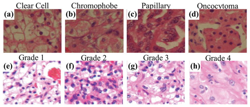
Sample histological tissue images for four renal tumor subtypes (a–d) and four Fuhrman grades (e–f). Images in (a–d) are taken from dataset 1 and have no grade information available, while images in (e–f) are various grades of clear cell samples taken from dataset 2.

B. Image features

We crop 512×512 pixel non-overlapping, adjacent tiles from the central portion of each image sample. We extract features from each tile, and unless mentioned otherwise, we average features over all tiles to represent the sample. We extract a comprehensive set of 2671 features from each sample. This set includes 12 feature subsets extracted from different processed forms of the original sample images.

Table I lists the 12 feature subsets and their combination set (i.e., the All set). Figure 2 describes the flow of feature extraction, where green boxes represent different forms of the processed image while pink boxes represent feature subsets. We generate the “Normalized Sample Image” using a color map quantile normalization method [4]. For the “Color Quantized Image”, we quantize the color space using self-organizing maps [5], [6] with the following parameters: 64 levels, I-by-64 grid size, linear initialization along the greatest Eigen vector, and ‘rectangular’ lattice type. The “Stain Segmented Image” is a four-level grayscale image, where gray-levels of 1, 2, 3 and 4 correspond to nuclear, red-blood cells, cytoplasmic and glandular structures respectively. These structures correspond to distinct H&E color stains and we segment them using an automatic color segmentation method [4]. We then extract binary masks for “Nuclear”, “Cytoplasmic” and “Glandular” structures in the image based on segmentation labels. We further segment the nuclear clusters in the nuclear mask into individual nuclei to produce the “Segmented Nuclei” [7], [8].

TABLE I.

LIST OF FEATURE SUBSETS, THEIR ACRONYMS AND EATURE COUNTS.

Feature Subset	Acronym	Count
Color	C	48
Global Texture	GT	565
Global Color Texture	GCT	493
Stain Texture	StT	503
Cytoplasmic Stain Objects’ shape	CStOS	249
Cytoplasmic Stain Texture	CStT	77
Glandular Objects’ Shape	GOS	249
Nuclear Stain Objects’ Shape	NStOS	249
Nuclear Stain Texture	NStT	77
Nuclear Stain Topology	NStTo	56
Nuclear Shape	NS	49
Nuclear Topology	NTo	56
All	A	2671

Figure 2.

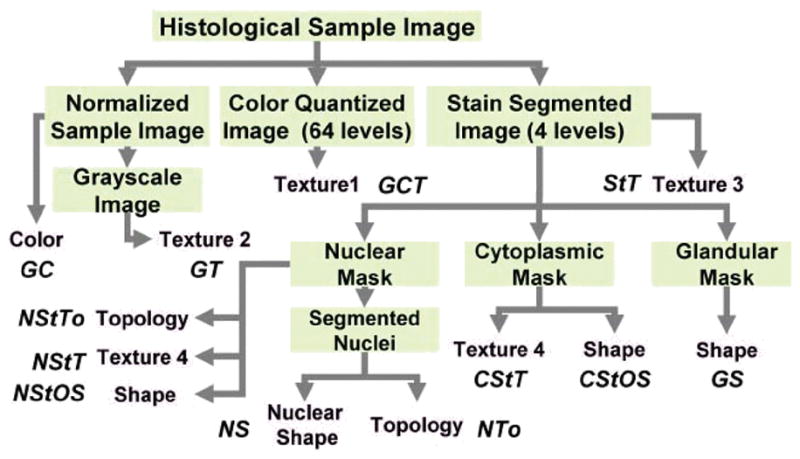
Flow diagram for image feature extraction. Green boxes: original or processed image. Pink boxes: feature subset. Pink box labels correspond to the following set of features—Color: R, G, and B histograms. Texture1: Haralick, Gabor, wavelet packet and multiwavelet. Texture2: Texture1, gray-level distribution and fractal. Texture3: Texture1 and stain co-occurrence. Texture4: Haralick and gray-level distribution. Shape: count, pixel area, convex hull area, solidity, perimeter, elliptical properties (area, major-minor axes lengths, eccentricity and orientation), boundary fractal, bending energy and Fourier reconstruction error. Topology: Delaunay triangle (area and side length), Voronoi diagram (area, side length and perimeter), minimum spanning tree edge length and closeness. Nuclear Shape: count, elliptical properties and cluster size.

The Color feature set corresponds to distributions of R, G, and B channel intensities with 16 bins per histogram [3]. The Texture1 feature set is a combination of Haralick, Gabor, wavelet packet and multiwavelet features. We extract and sum 64-level GLCM matrices over all tiles. Thereafter, we extract 13 Haralick features from the summed GLCM matrix [9]. We generate 28 unique Gabor filters for different values of sinusoid frequency, f, and orientation, θ[10]. We consider θ={0,π/4,π/2,3π/4} radians and $f\in \{\sqrt{2}/256,\sqrt{2}/128,\sqrt{2}/64,\sqrt{2}/32,\sqrt{2}/16,\sqrt{2}/8,\sqrt{2}/4\}$ cycles per pixel. We calculate energy (E) and entropy (H) [1] of each Gabor filter response image giving 56 features per tile. We perform wavelet packet decomposition of the grayscale image using ‘db6’ and ‘db20’ wavelets [11]. We extract level-3 sub-matrices (total 64 sub-matrices per wavelet type) for each tile and then extract energy and entropy [1] of these sub-matrices. This results in 256 features per tile. We also perform a two-level multiwavelet transform of the grayscale image with multiwavelets-GHM, SL and SA4 [1]. We obtain 28 sub-matrices per multiwavelet type and calculate their energy and entropy resulting in 168 features per tile. The Texture2 feature set is a combination of Texture1 features, gray-level distribution, and fractal features. Gray-level distribution captures the distribution of gray-levels in a grayscale image using 64 bins in the histogram. We extract eight fractal dimensions for the grayscale image using the method described by Huang and Lee [2]. The Texture3 feature set is a combination of Texture1 features and stain co-occurrence features. Stain co-occurrence captures the frequency of adjacent stains in a histological image [12]. The Texture4 feature set is a combination of gray-level distribution and Haralick features applied to specific stains. We capture the grayscale texture of the cytoplasmic or nuclear stain areas in the grayscale image bounded by their respective masks. The Shape feature set captures shape properties of the structures in three segmentation masks. Among the structures identified by segmentation, we eliminate noise using a 20-pixel area threshold. The description for pixel area, convex hull area, solidity, perimeter, elliptical properties (area, major-minor axes lengths, eccentricity and orientation) and bending energy is available in [13]. We extract boundary fractal dimension, using box counting on a binary object image. We extract Fourier shape descriptor error (i.e., RMS error) in reproducing the shape using 1, 2, …, 20 harmonics [14]. We estimate the distribution of each of the 31 measures over the objects in all the tiles. We then represent this distribution using eight statistics: mean, median, minimum, maximum, standard deviation, inter-quartile range, skewness and kurtosis. In addition to these features, we also use object count as a feature. Therefore, the Shape feature set consists of 249 features. We extract Topology features using elliptical centers from unsegmented nuclear stain objects and segmented individual nuclei. We extract topology features by measuring properties of spatial graphs such Deluanay triangulation (areas and side lengths), Voronoi diagram (area, side length and perimeter) and minimum spanning tree side lengths [15]. We also measure object closeness, which is the average distance of an object to its five closest neighbors [7]. We represent the distribution of these seven topology measures for a single image using the same eight statistics used for Shape features, resulting in 56 features. The Nuclear Shape feature set is a combination of nucleus count, elliptical properties (the same as those of Shape features) and cluster size. Cluster size measures the number of nuclei in a cluster. Because it is a distribution, we estimate the same eight statistics as object shape features.

C. Feature selection and classification

In this study, we consider all binary endpoints comparing pairs of classes. Both grading and subtyping datasets have 4 classes and 6 endpoints. We develop classification models for all combinations of binary endpoint (total of 12) and feature subset (total of 13, Table I). We consider four classification methods (Bayesian, Logistic Regression, k-NN and Linear SVM) with a fixed set of parameters. For Bayesian, we consider both pooled and un-pooled variance with spherical and diagonal variance matrices. For k-NN, we consider ten values from 1 to 10. For SVM, we consider 28 cost values (0.1:0.1:0.9, 1:1:9, and 10:10:100 (start value: step: end value)). Logistic regression has no additional parameters. For each classifier model, we consider five feature selection techniques including t-test, Wilcoxon rank sum test, Significance Analysis of Microarrays (SAM) [16], and two types of mRMR (Minimum redundancy and maximum relevance): mRMR-d (difference) and mRMR-q (quotient) [17]. We consider 45 feature sizes ranging from 1 to 45. Thus, for each combination of endpoint and feature subset, we use cross validation to find optimal classification models from among 9,675 models. We identify optimal classification models for each endpoint using stratified nested cross-validation with 10 iterations and 5 folds in both the outer and inner cross-validation. The inner cross-validation is used for identifying optimal model parameters (i.e., feature selection method, feature size, classifier, and classifier parameters). The performance of each optimal model is then assessed using the testing set from outer cross-validation. We select the simplest classification models that are within one standard deviation of the best performing model. The simplest models are defined as those with the smallest feature size, highest k for k-NN models, and smallest cost for SVM models. For Bayesian models, we prefer pooled over unpooled covariance and spherical over diagonal covariance. We have not assigned any preference to any particular classification method or feature selection method. Therefore, for each combination of endpoint and feature set, it is possible to obtain multiple optimal models. In such cases, we report the average performance of all models.

Section III. Results and Discussion

A. Classification results and emergent feature subsets

We optimize and validate models for every combination of feature subset and binary endpoints (both subtyping and grading endpoints). Table II lists average outer cross-validation accuracy over 10 iterations and 5-folds. It can be observed that all subtyping models based on the All subset, with the exception of CH vs. CC and CH vs. ON, perform with an average accuracy > 90%. Low performance of these two endpoints is supported by the literature, as histologically and genetically, CH is similar to CC and ON. Among grading endpoints, binary comparisons of grades differing by two or more levels tend to perform better. Intuitively, this makes sense because with greater difference in grades, there are more visually apparent changes. It is interesting that the All subset is never the best performing subset. The gap between the best performing feature set and the All set is larger for grading endpoints. This is probably because, with the large feature list and fewer samples in the grading dataset, it is more likely that a model over fits. Hence, it is important to identify statistically important feature sets for an endpoint. We investigate the importance of feature subsets using a method normally used to identify over- represented Gene Ontology terms in a list of genes [18]. For each endpoint, we consider all optimal classification models that select features from the entire set of 2671 image features. We count the number of features drawn from each of the 12 feature subsets and use a one-sided Fisher’s exact test to determine if any of the feature subsets are statistically over-represented at a p-value threshold of 0.01 (adjusted for multiplicity using the Bonferroni method). A small p-value for a subset indicates that the number of features selected from that subset is higher than what is expected by random chance. In Table II, for each endpoint, we highlight feature subsets that are statistically over-represented. It can be observed that over-represented feature subsets tend to correspond to the best performing subsets for each endpoint.

TABLE II.

CROSS-VALIDATION ACCURACY OF BINARY SUBTYPING AND GRADING DIAGNOSTIC MODELS BASED ON DIFFERENT FEATURE SUBSETS AND STATISTICALLY OVER-REPRESENTED FEATURE SUBSETS.

Feature Subset	CH vs. CC	CH vs. ON	CH vs. PA	CC vs. ON	CC vs. PA	ON vs. PA	G1 vs. G2	G1 vs. G3	G1 vs. G4	G2 vs. G3	G2 vs. G4	G3 vs. G4
A	0.77	0.79	0.92	0.94	0.91	0.96	0.51	0.81	0.79	0.62	0.62	0.59
C	0.81	0.69	0.92	0.84	0.96	0.79	0.70	0.58	0.62	0.46	0.56	0.62
GT	0.84	0.62	0.89	0.92	0.91	0.77	0.47	0.51	0.74	0.43	0.63	0.66
GCT	0.65	0.65	0.84	0.65	0.86	0.84	0.52	0.54	0.65	0.49	0.55	0.51
StT	0.68	0.60	0.89	0.73	0.91	0.75	0.62	0.56	0.63	0.42	0.67	0.55
CStOS	0.77	0.63	0.48	0.60	0.66	0.58	0.44	0.48	0.59	0.52	0.68	0.63
CStT	0.73	0.64	0.86	0.70	0.80	0.81	0.48	0.43	0.62	0.50	0.54	0.59
GOS	0.69	0.72	0.70	0.92	0.88	0.74	0.44	0.55	0.49	0.44	0.44	0.44
NStOS	0.68	0.71	0.94	0.93	0.75	0.93	0.41	0.84	0.59	0.73	0.48	0.45
NStT	0.58	0.70	0.82	0.55	0.87	0.85	0.48	0.65	0.61	0.45	0.65	0.51
NStTo	0.73	0.76	0.60	0.58	0.56	0.74	0.37	0.45	0.49	0.45	0.47	0.47
NS	0.71	0.67	0.88	0.97	0.82	0.98	0.61	0.81	0.84	0.68	0.82	0.59
NTo	0.78	0.82	0.89	0.58	0.71	0.71	0.48	0.59	0.61	0.46	0.59	0.48

B. Biological Interpretation

Eble et al. provide guidelines for subtyping renal tumors [19]. Here, we can relate these biological properties to the feature subsets as follows. CH, with its wrinkled nuclei, granular cytoplasm and perinuclear halos, differs from other subtypes in nuclear, texture, and glandular object features. This may explain why the NS, NStOS, GT and GOS feature subsets are selected as statistically important subsets for endpoints with CH. Due to clear cytoplasm, CC differs from other subtypes in terms of color, glandular objects and texture. Thus, the C, GT and GOS feature subsets tend to emerge for endpoints with CC. Due to nuclear clusters, PA differs from other subtypes in terms of nuclear properties represented by the NS, NStT, and NStOS feature subsets. Finally, due to its compact nuclear nests, ON differs from CH in terms of topology, represented by the NStTo. Similarly, renal cancer is graded using the Fuhrman nuclear grading system [19]. Therefore, we observe nuclear shape features and nuclear mask features are the most important feature sets for renal cancer grading.

Section IV. Conclusion

We have developed a system with a comprehensive set of existing image features that can be applied to a wide variety of histological diagnosis applications. The comprehensive set includes 12 feature subsets that capture various histological image properties. We assessed the predictive performance of the system by applying it to several renal tumor subtyping and grading endpoints. We also evaluated the contribution of feature subsets to each disease endpoint in order to reveal emergent properties in the histological images that may relate to biological properties. Results indicate that the feature sets that emerge from the system are biologically interpretable.

References

- 1.Jafari-Khouzani K, Soltanian-Zadeh H. Multiwavelet grading of pathological images of prostate. IEEE Transactions on Biomedical Engineering. 2003;50:697–704. doi: 10.1109/TBME.2003.812194. [DOI] [PubMed] [Google Scholar]
- 2.Huang PW, Lee CH. Automatic classification for pathological prostate images based on fractal analysis. Medical Imaging IEEE Transactions on. 2009;28:1037–1050. doi: 10.1109/TMI.2009.2012704. [DOI] [PubMed] [Google Scholar]
- 3.Tabesh A, et al. Multifeature prostate cancer diagnosis and Gleason grading of histological images. IEEE Transactions on Medical Imaging. 2007;26:1366–1378. doi: 10.1109/TMI.2007.898536. [DOI] [PubMed] [Google Scholar]
- 4.Kothari S, et al. Automatic batch-invariant color segmentation of histological cancer images. IEEE International Symposium on Biomedical Imaging: From Nano to Macro; 2011; pp. 657–660. [DOI] [PMC free article] [PubMed] [Google Scholar]
- 5.Vesanto J, et al. Self-organizing map in Matlab: the SOM toolbox. Proceedings of the Matlab DSP Conference; 1999; pp. 16–17. [Google Scholar]
- 6.Sertel O, et al. Histopathological image analysis using model-based intermediate representations and color texture: Follicular lymphoma grading. Journal of Signal Processing Systems. 2009;55:169–183. [Google Scholar]
- 7.Kothari S, et al. Extraction of informative cell features by segmentation of densely clustered tissue images. International Conference of the IEEE Engineering in Medicine and Biology Society; 2009; pp. 6706–6709. [DOI] [PMC free article] [PubMed] [Google Scholar]
- 8.Kothari S, et al. Automated cell counting and cluster segmentation using concavity detection and ellipse fitting techniques. IEEE International Symposium on Biomedical Imaging: From Nano to Macro; 2009; pp. 795–798. [DOI] [PMC free article] [PubMed] [Google Scholar]
- 9.Haralick RM, et al. Textural features for image classification. Systems Man and Cybernetics IEEE Transactions on. 1973;3:610–621. [Google Scholar]
- 10.Jain AK, Farrokhnia F. Unsupervised texture segmentation using Gabor filters. Pattern recognition. 1991;24:1167–1186. [Google Scholar]
- 11.Laine A, Fan J. Texture classification by wavelet packet signatures. IEEE Transactions on Pattern Analysis and Machine Intelligence. 1993;15:1186–1191. [Google Scholar]
- 12.Chaudry Q, et al. Automated Renal Cell Carcinoma Subtype Classification Using Morphological, Textural and Wavelets Based Features. Journal of Signal Processing Systems. 2009;55:15–23. doi: 10.1007/s11265-008-0214-6. [DOI] [PMC free article] [PubMed] [Google Scholar]
- 13.Boucheron L. PhD thesis. University of California; Santa Barbara: 2008. Object-and spatial-level quantitative analysis of multispectral histopathology images for detection and characterization of cancer. [Google Scholar]
- 14.Kuhl F, Giardina C. Elliptic Fourier features of a closed contour. Computer graphics and image processing. 1982;18:236–258. [Google Scholar]
- 15.Doyle S, et al. Automated grading of breast cancer histopathology using spectral clustering with textural and architectural image features. IEEE International Symposium on Biomedical Imaging: From Nano to Macro; 2008; pp. 496–499. [Google Scholar]
- 16.Tusher VG, et al. Significance analysis of microarrays applied to the ionizing radiation response. Proceedings of the National Academy of Sciences. 2001;98:5116. doi: 10.1073/pnas.091062498. [DOI] [PMC free article] [PubMed] [Google Scholar]
- 17.Peng H, et al. Feature selection based on mutual information: criteria of max-dependency, max-relevance, and min-redundancy. IEEE Transactions on Pattern Analysis and Machine Intelligence. 2005:1226–1238. doi: 10.1109/TPAMI.2005.159. [DOI] [PubMed] [Google Scholar]
- 18.Zeeberg BR, et al. GoMiner: a resource for biological interpretation of genomic and proteomic data. Genome Biol. 2003;4:R28. doi: 10.1186/gb-2003-4-4-r28. [DOI] [PMC free article] [PubMed] [Google Scholar]
- 19.Eble J, et al. Pathology and genetics of tumours of the urinary system and male genital organs. IARC press; Lyon: 2004. [Google Scholar]