Stochastic models of gene transcription with upstream drives: exact solution and sample path characterization

Abstract

Gene transcription is a highly stochastic and dynamic process. As a result, the mRNA copy number of a given gene is heterogeneous both between cells and across time. We present a framework to model gene transcription in populations of cells with time-varying (stochastic or deterministic) transcription and degradation rates. Such rates can be understood as upstream cellular drives representing the effect of different aspects of the cellular environment. We show that the full solution of the master equation contains two components: a model-specific, upstream effective drive, which encapsulates the effect of cellular drives (e.g. entrainment, periodicity or promoter randomness) and a downstream transcriptional Poissonian part, which is common to all models. Our analytical framework treats cell-to-cell and dynamic variability consistently, unifying several approaches in the literature. We apply the obtained solution to characterize different models of experimental relevance, and to explain the influence on gene transcription of synchrony, stationarity, ergodicity, as well as the effect of time scales and other dynamic characteristics of drives. We also show how the solution can be applied to the analysis of noise sources in single-cell data, and to reduce the computational cost of stochastic simulations.

1. Introduction

Gene transcription, the cellular mechanism through which DNA is copied into mRNA transcripts, is a complex, stochastic process involving small numbers of molecules [1]. As a result, the number of mRNA copies for most genes is highly heterogeneous over time within each cell, and across cells in a population [2–4]. Such fundamental randomness is biologically relevant: it underpins the cell-to-cell variability linked with phenotypic outcomes and cell decisions [5–9].

The full mathematical analysis of gene expression variability requires the solution of master equations. Given a gene transcription model, its master equation (ME) is a differential–difference equation that describes the evolution of P(n, t), the probability of having n mRNA molecules in a single cell at time t. However, MEs are problematic to solve, both analytically and numerically, due to the difficulties associated with discrete stochastic variables—the number of molecules n is an integer [10]. Most existing analytical solutions of the ME are specific to particular models and are typically obtained via the probability generating function under stationarity assumptions [11–15]. A few other solutions include the decaying time dependence describing the relaxation transient towards stationarity from a given initial distribution [16–19]. In the usual situation when analytical solutions are intractable, the first few moments of the distribution are approximated, usually at stationarity, although error bounds are difficult to obtain under closure schemes [20,21]. Alternatively, full stochastic simulations are used, yet the computational cost to sample P(n, t) at each t is often impractical, and many methods lead to estimation bias in practice [22].

The emergence of accurate time-course measurements of mRNA counts in single cells [3,4,23–25] has revealed the high dynamic variability of gene expression both at the single-cell and population levels. This variability has several sources. Cells express genes heterogeneously [4,26] and hence models need to capture intercellular variability; but cells are also subjected to time-varying inputs of a stochastic and/or deterministic nature, either from their environment or from regulatory gene networks inside the cell. Therefore, standard ME models with stationary solutions, which also tacitly assume that gene expression is uncorrelated between cells, cannot capture fully such sources of variability. Mathematically, ME models must be able to describe time-dependent gene transcription in single cells within an inhomogeneous population, i.e. they must allow a varying degree of synchrony and of cell-to-cell variability across the population. In addition, they must be able to account for non-stationary dynamic variability due to upstream biological drives, such as circadian rhythms and cell cycle [27,28], external signalling [29], or stimulus-induced modulation or entrainment [30,31].

Recent techniques to model cell-to-cell correlations have used the marginalization of extrinsic components [32], mixed-effects models [33] or deterministic rate parameters [34]. Several of the results correspond to deterministic rates and are well known in queuing theory [35]. However, full solutions of the ME that capture temporal heterogeneity as well as variability in parameters, from the single-cell to the population level, are yet to be explored, and could help unravel in conjunction with experiments how the dynamics of upstream drives within a biological network affect gene transcription.

Here, we consider a simple, yet generic, framework for the solution of the ME of gene transcription and degradation for single cells under upstream drives, i.e. when the transcription and degradation parameters are time-dependent functions or stochastic variables. We show that the exact solution P(n, t) for such a model naturally decouples into two parts: a discrete transcriptional Poissonian downstream component, which is common to all transcription models of this kind, and a model-specific continuous component, which describes the dynamics of the parameters reflecting the upstream variation. To obtain the full solution P(n, t), one only needs to calculate the probability density for the model-specific upstream drive, which we show corresponds to a continuous variable satisfying a linear random differential equation directly related to traditional differential rate equations of chemical kinetics. Our results can thus be thought of as a generalization of the Poisson representation [36,37] (originally defined as an ansatz with constant rate parameters) to allow for both time-varying and stochastic rates in transcription–degradation systems. Our work also departs from the work of Jahnke & Huisinga [34] by allowing the presence of cell-to-cell variability (or uncertainty) in the dynamical drive.

Below, we present the full properties of the general solution, and we derive the relationship of the observable time-varying moments with the moments of the dynamic upstream component. Because our framework treats dynamic and population variability consistently, we clarify the different effects of variability in the drives by considering the Fano factor across the population and across time. To illustrate the utility of our approach, we present analytical and numerical analyses of several models from the literature, which are shown to simply correspond to different upstream drives, deterministic or stochastic. These examples highlight our modelling approach: a flexible solvable model with upstream dynamic variability, reflecting the generic hypothesis that experimentally observed outputs are usually driven by fluctuating, usually unmeasurable and uncertain, upstream intra- and extracellular signals. Our framework provides a means to characterize such upstream variability, dynamical and population-wide, and we provide examples of its use for computational biology and data analysis in relation to experiments.

2. The master equation for gene transcription in populations of cells with upstream drives

2.1. Notation and formulation of the problem

To study gene expression in a single cell with time-dependent upstream drives, we consider the stochastic process in continuous time t, , where N_t is a discrete random variable describing the number of mRNA molecules in the cell. We look to obtain the probability mass function, P(n, t)≔Pr(N_t = n).

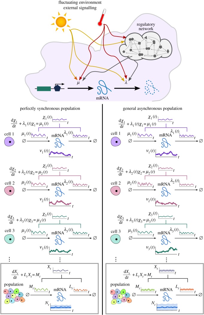
The mRNA copy number increases via transcription events and decreases via degradation events but, importantly, we acknowledge that the observed gene reflects the dynamic variability of intra- and extracellular processes and that cells are heterogeneous. Thus, the transcription and degradation rates can depend on time and can be different for each cell (figure 1). To account for such variability, we describe transcription and degradation rates as stochastic processes and , without specifying any functional form except requiring that M and L do not depend on the number of mRNA molecules already present. Deterministic time-varying transcription–degradation rates, with or without cell-to-cell correlations, are a particular case of this definition.

Figure 1.

Single-cell gene transcription under upstream drives. The transcription of each cell i takes place under particular cellular drives and , representing time-varying transcription and degradation rates. Both cellular drives are combined into the upstream effective drive , which dictates the long-term probability distribution describing the stochastic gene expression within each cell (2.10). When there is cell-to-cell variability in the population, the cellular drives are described by processes M and L leading to the upstream effective drive X. The probability distribution of the population corresponds to the mixture of the upstream process X and the Poissonian downstream transcriptional component, as given by (2.14). Increased synchrony in the population implies decreased ensemble variability of the random variables M_t, L_t, X_t and N_t. (Online version in colour.)

Following standard notation in the stochastic processes literature, M_t and L_t denote the random variables at time t. To simplify notation, however, we depart from standard notation and denote the sample paths (i.e. realizations) of M and L by and , respectively, thinking of them as particular functions of time describing the transcription and degradation rates under the changing cellular state and environmental conditions in an ‘example’ cell (figure 1). The sample paths of other random variables are denoted similarly, e.g. the sample paths of N_t are .

The sample paths and represent cellular drives encapsulating the variability across time and across the population consistently. This formulation unifies several models in the literature, which implicitly or explicitly assume time-varying transcription and/or degradation processes [4,16,38–42], and can be shown to correspond to particular types of dynamic upstream variability. In addition, the framework allows us to specify cell-to-cell correlations across the population, which we refer to as the ‘degree of synchrony’. A population will be perfectly synchronous when the sample paths of the drives for every cell in the population are identical, i.e. if M_t and L_t have zero variance. If, however, transcription and/or degradation rates differ between cells, M_t and L_t themselves emerge from a probability density: the wider the density, the more asynchronous the cellular drives (figure 1).

Our aim is to obtain the probability distribution of the copy number N_t under upstream time-varying cellular drives M_t and L_t, themselves containing stochastic parameters reflecting cell-to-cell variability. We proceed in two steps: first, we obtain the solution for the perfectly synchronous system without cell-to-cell variability; then we consider the general asynchronous case.

2.2. Perfectly synchronous population

As a first step to the solution of the general case, consider a population of cells with perfectly synchronous transcription and degradation rate functions, and ; i.e. the transcription and degradation processes are defined by the same sample path for the whole population and the stochastic processes M and L have zero variance at all times (figure 1).

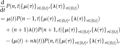
In the perfectly synchronous case, we have an immigration–death process with reaction diagram

2.1

and its ME is standard:

2.2

where denotes the probability of having n mRNAs at time t for the given history of the cellular drives and .

Using the probability generating function

we transform the ME (2.2) into

Without loss of generality, let us first consider an initial condition with n₀ mRNA molecules. Using the method of characteristics, we obtain the solution

2.3

which is given in terms of

2.4

We will refer to the time-varying continuous function χ(t) as the effective drive, as it integrates the effect of both cellular drives.

Note that solution (2.3) can be rewritten as the product of two probability generating functions:

corresponding to a binomial and a Poisson distribution, respectively. Hence, for the perfectly synchronous case, the solution is given by

2.5

2.6

2.7

where is a binomial random variable with n₀ trials and success probability , and is a Poisson random variable with parameter χ(t). The physical interpretation of this breakdown is that describes the mRNA transcripts that were initially present in the cell and still remain at time t, whereas describes the number of mRNAs transcribed since t = 0.

Since and are independent, it is easy to read off the first two moments directly:

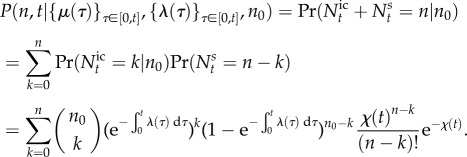
From (2.5)–(2.7), the full distribution is

2.8

This mathematical form is well known when the rates are constant [37,43], and a classical result in queueing theory [35]. We also remark that the solution with time-dependent rates (2.8) is the one-gene case of the main result in Jahnke & Huisinga [34].

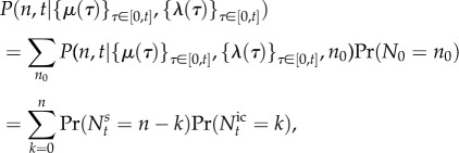
If the initial state is itself described by a random variable N₀ with its own probability distribution, we apply the law of total probability to obtain the solution in full generality as follows (see appendix A):

2.9

where is distributed according to (2.5)–(2.7), and is the mixture of the time-dependent binomial distribution (2.5) and the distribution of the initial condition N₀.

2.2.1. The initial transient ‘burn in’ period

For biologically realistic degradation rates , the contribution from the initial condition () decreases exponentially. Hence, as time grows, the transcripts present at t = 0 degrade, and the population is expected to be composed of mRNAs transcribed after t = 0.

If the initial distribution of N₀ is not the stationary distribution of the ME (or, more generally, not equal to the attracting distribution of the ME, as defined in appendix A), there is an initial time dependence of P(n, t) lasting over a time scale T^ic (given by ), which corresponds to a ‘burn-in’ transient associated with the decay of the initial condition. We remark that the time-dependence described in [16–19] corresponds only to this ‘burn-in’ transient (see also figure 7).

Figure 7.

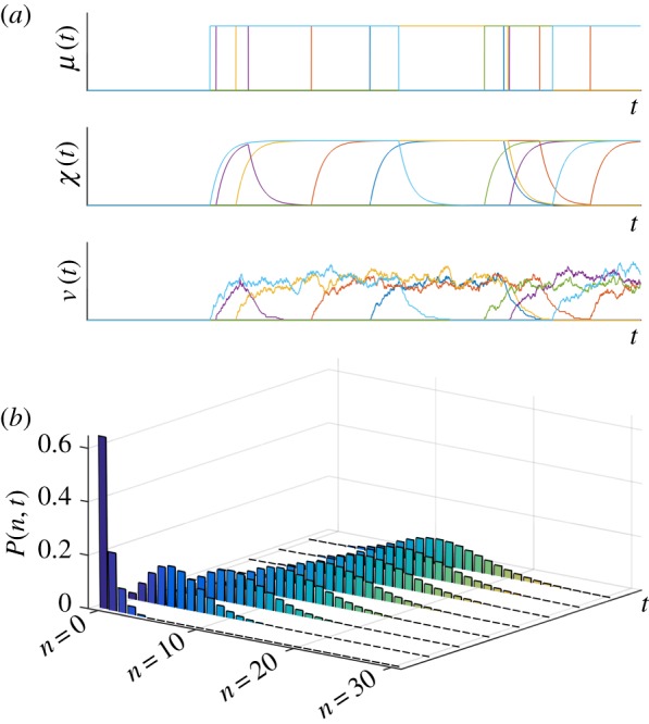
‘Burn-in’ transient in the RT model. (a) Sample paths of the transcription rate M, the effective upstream drive X and the number of mRNAs N for an initial condition P(0, 0) = 1 with all cells initialized in the inactive state [16]. (b) The full solution of the RT model for this initial probability distribution exhibits an exponential decay as the system approaches its stationary distribution. The delta distribution at t = 0 is omitted for scaling purposes. (Online version in colour.)

On the other hand, when the initial distribution of N₀ is the stationary distribution (or the attracting distribution) of the ME, the component containing the initial condition () and the long-term component () balance each other at every point in time, maintaining stationarity (or the attracting distribution), as shown analytically in appendix A.

2.2.2. The long-term behaviour of the solution

In this work, we focus on the time dependence of P(n, t) induced through non-stationarity of the parameters and/or correlated behaviour of the cells within the population. Hence, for the remainder of the paper, we neglect the transient terms. Consequently, for perfectly synchronous cellular drives, the solution of the ME (2.2) is a Poisson random variable with time-dependent rate equal to the effective upstream drive, χ(t):

with distribution

2.10

which makes explicit the dependence on the history of the sample paths , which is encapsulated in the value of the effective drive χ(t) at time t.

Indeed, from (2.4) it follows that the sample path satisfies a first-order linear ordinary differential equation with time-varying coefficients:

2.11

which is the rate law for a chemical reaction with zeroth-order production with rate μ(t), and first-order degradation with rate λ(t) per mRNA molecule. For biologically realistic (i.e. positive and finite) cellular drives, χ(t) is a continuous function.

2.3. The general asynchronous case: cell-to-cell variability in the cellular drives

Consider now the general case where different sample paths for the cellular drives are possible, i.e. we allow explicitly for the transcription and degradation rates to vary from cell to cell. The cell population will have some degree of asynchrony, hence M_t and L_t have non-zero variance for at least some t ≥ 0. The transcription and degradation rates are then described by stochastic processes M and L:

2.12

and the collection of all differential equations of the form (2.11) is represented formally by the random differential equation¹

2.13

Equations of this form appear in many sciences, and a large body of classical results allows us to determine f_Xt(x, t) the probability density function of the upstream process X_t [44–46]. Below, we use such results to obtain for biologically relevant models.

Note that from equation (2.10) and the law of total probability, it follows that the probability mass function for the random variable N_t under cellular drives described by the random processes M and L is given by the Poisson mixture (or compound) distribution:

2.14

where the density of the effective drive X_t (to be determined) can be understood as a mixing density. The notation recalls explicitly the dependence of the solution on the density of X_t, but we drop this reference and use P(n, t) below to simplify notation. The problem of solving the full ME is thus reduced to finding the mixing density . Note that, for synchronous drives, we have , where δ is the Dirac delta function, and (2.14) reduces to (2.10).

Equation (2.14) also shows that there are two separate sources of variability in gene expression, contributing to the distribution of N_t. One source of variability is the Poisson nature of transcription and degradation, common to every model of the form considered here; the second source is the time variation or uncertainty in the cellular drives, encapsulated in the upstream process X_t describing the ‘degree of synchrony’ between cells and/or their variability over time. In this sense, equation (2.14) connects with the concept of separable ‘intrinsic’ and ‘extrinsic’ components of gene expression noise pioneered by Swain et al. [47–50]. Yet rather than considering moments, the full distribution P(n, t) is separable into a model-dependent ‘upstream component’ given by , and a downstream transcriptional ‘Poisson component’ common to all models of this type.

3. The effective upstream drive in gene transcription models

The generic model of gene transcription and degradation with time-dependent drives introduced above provides a unifying framework for several models previously considered in isolation. In this section, we exemplify the tools to obtain the density of the effective drive analytically or numerically through relevant examples.

3.1. Gene transcription under upstream drives with static randomness

In this first section, we consider models of gene transcription where the upstream drives are deterministic, yet with random parameters representing cell variability.

3.1.1. Random entrainment to upstream sinusoidal drives: random phase offset in transcription or degradation rates

Equation (2.13) can sometimes be solved directly to obtain from a transformation of the random variables M_t and L_t. We now show two such examples, where we explore the effect of entrainment of gene transcription and degradation to an upstream periodic drive [51].

First, consider a model of gene transcription of the form (2.12) with a transcription rate given by a sinusoidal function and where each cell has a random phase. This random entrainment (RE) model is a simple representation of a cell population with transcription entrained to an upstream rhythmic signal, yet with a random phase offset for each cell:

3.1

where m and ω are given constants and Φ is a (static) random variable describing cell-to-cell variability (or uncertainty). Solving equation (2.13) in this case, we obtain

where , B = m/2 and .

Suppose Φ* is uniformly distributed on [−r, r], r ≤ π. Inverting the sine with Φ* restricted to [−r, r], we obtain

3.2

where is the number of solutions of for . As the phase distribution of the drives becomes narrower, the upstream variability disappears: . In this limit, all cells follow the entraining drive exactly, and P(n, t) becomes a Poisson distribution at all times.

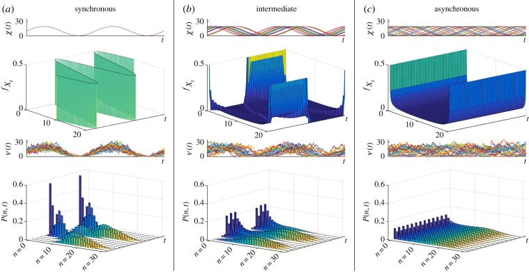
Figure 2 depicts for r = 0 (no cell-to-cell phase variation, figure 2a and for r = π/2, and r = π (increasingly wider uniform distribution of phases, figure 2b,c). The full distribution P(n, t) is obtained using (3.2) and (2.14).

Figure 2.

Gene transcription under the RE model (3.1) with constant degradation rate and transcription rates entrained to an upstream sinusoidal signal with ω = 1. Each cell has a random phase offset ϕ drawn from a distribution. (a) The synchronous population corresponds to identical phases across the population. In this case, the transcription reflects the time variability of the upstream drive mixed with the stochasticity due to the downstream Poisson process of transcription. When the random phases ϕ are uniformly distributed on an interval of range (b) π and (c) 2π, the population becomes increasingly asynchronous. For all three cases, we show (top to bottom): sample paths of the effective drive, X; its density given by equation (3.2); sample paths of the number of mRNAs, N; and the full solution of the ME P(n, t). (Online version in colour.)

Second, let us consider the same model of entrainment to an upstream sinusoidal signal with a random offset, but this time via the degradation rate:

3.3

where m, a, b and ω are given constants, and Φ is a (static) random variable.

Equation (2.13) can be solved approximately [51] to give

where , and . As before, if Φ* is uniform on [−r, r], r ≤ π, the density of the effective drive takes the same form (3.2) as above.

3.1.2. Upstream Kuramoto promoters with varying degree of synchronization

As an illustrative computational example, we study a population of cells whose promoter strengths display a degree of synchronization across the population. To model this upstream synchronization, consider the Kuramoto promoter model, where the promoter strength of each cell i depends on an oscillatory phase θ_i(t), and cells are coupled via a Kuramoto model [52–54]. We then have a model of the form (2.12) with

3.4

Here m and b are constants and are the phase variables for the C cells governed by the globally coupled Kuramoto model:

3.5

where K is the coupling parameter and the intrinsic frequency of each cell, ω_i, is drawn from the random distribution . The Kuramoto model allows us to tune the degree of synchrony through the coupling K: for small K, the cells do not display synchrony since they all have a slightly different intrinsic frequency; as K is increased, the population becomes more synchronized.

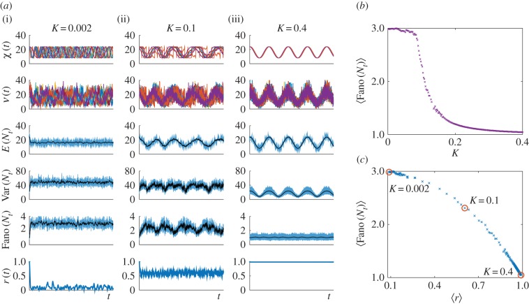
This model is a simple representation of nonlinear synchronization processes in cell populations with intrinsic heterogeneity [55–58]. In figure 6a, we show how the sample paths change as the degree of synchrony increases, and we exemplify the use of (2.14) for the numerical solution of the gene expression of this model.

Figure 6.

Noise characteristics of the Kuramoto promoter model (3.4). (a) Numerical simulations for C = 100 oscillatory cells and different coupling parameters: K = 0.002, 0.1, 0.4 ((i), (ii), (iii), respectively). For each coupling, the sample paths of the upstream effective drive X and mRNA counts N are shown. The mean, variance and ensemble Fano factor of N were calculated from the sample paths of N (blue lines) and, more efficiently, from the sample paths of X (black lines). The last row shows the Kuramoto order parameter r(t) measuring the cell synchrony, signalled by . (b) Ensemble Fano factor (averaged over the simulated time courses) against coupling parameter . As K is increased, the oscillators become synchronized and the ensemble Fano factor decreases towards the Poisson value of unity. (c) Scatter plot of the ensemble Fano factor against the order parameter r(t) (both averaged over the simulated time courses). As the oscillators become synchronized (), the ensemble Fano factor also approaches 1, signifying that the distribution is Poisson at all times. (Online version in colour.)

3.2. Asynchronous transcription under stochastic multistate promoters

In the previous section, we obtained by capitalizing on the precise knowledge of the sample paths of M and L to solve (2.13) explicitly. In other cases, we can obtain by following the usual procedure of writing down an evolution equation for the probability density of an expanded state that is Markovian, followed by marginalization. More specifically, let the vector process Y prescribe the upstream drives, so that and , and consider the expanded state . Note that since Y is upstream, it prescribes X (and not vice versa). We can then write the evolution equation for the joint probability density :

3.6

which follows from conservation of probability. In equation (3.6), the differential operator for X, which follows from (2.13), is the first jump moment [59] conditional upon Y_t = y (and hence upon and ); the second term is the infinitesimal generator of the upstream processes. In particular, for continuous stochastic processes is of Fokker–Planck type, and for Markov chains is a transition rate matrix. The desired density can then be obtained via marginalization.

Equation (3.6) can be employed to analyse the widely used class of transcription models with asynchronous, random promoter switching between discrete states, where each state has different transcription and degradation rates representing different levels of promoter activity due to, for example, transcription factor binding or chromatin remodelling [40]. A classic example is the random telegraph (RT) model, first used by Ko in 1991 [60] to explain cell-to-cell heterogeneity and bursty transcription (figure 3a).

Figure 3.

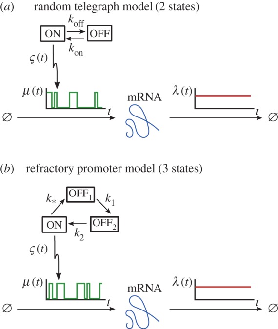
Asynchronous stochastic promoter switching models correspond to upstream stochastic processes. The promoter cycles between the discrete states, transitioning stochastically with rates as indicated: (a) the standard 2-state random telegraph model; (b) the 3-state refractory promoter model. (Online version in colour.)

In our framework, such random promoter switching can be understood as an upstream stochastic process driving transcription as follows. Let us assume that the promoter can attain D states s, and each state has constant transcription rate m_s and constant degradation rate . The state of the promoter is described by a random process , with sample paths denoted by , and its evolution is governed by the D-state Markov chain with transition rate k_sr from state r to state s. The state of the promoter S_t = s prescribes that M_t = m_s and . Hence, the sample paths of M and L are a succession of step functions with heights m_s and , respectively, occurring at exponentially distributed random times.

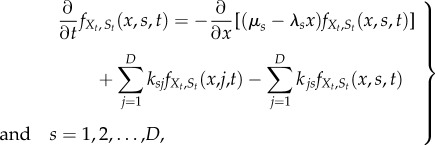
As described above, we expand the state space of the cellular drives to include the promoter state . The evolution equation (3.6) is then given by D coupled equations:

3.7

which can be thought of as a set of multistate Fokker–Planck–Kolmogorov equations [59]. Marginalization then leads to the density of the effective drive:

3.8

and the full ME solution is obtained from (3.8) and (2.14).

We illustrate this approach more explicitly with two examples (figure 3): a rederivation of the known solution of the standard RT model; and the solution of the 3-state cyclic model with a refractory state. Results for other promoter architectures are discussed in [61].

3.2.1. The random telegraph model (2 states)

Although the RT model has been solved by several methods [16,38,39], we briefly rederive its solution within the above framework to clarify its generalization to other promoter architectures.

Consider the standard RT model (figure 3a), with promoter switching stochastically between the active state s_on = 1, with constant transcription rate m₁ = m, and the inactive state s_off = 0, where no transcription takes place, m₀ = 0. The transition rates between the two states are k₁₀ = k_on and k₀₁ = k_off. Without loss of generality, we assume . The transcription model is of the form (2.12) with

3.9

where with waiting times drawn from exponential distributions: and .

Let , and let us denote and , with . Then the multistate Fokker–Planck–Kolmogorov equations (3.7) are

with integral conditions and .

At stationarity, it then follows [62] that

3.10

where is the Beta function. In other words, at stationarity, the normalized effective drive is described by a Beta distribution:

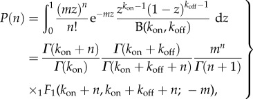
Using (3.10) and (2.14), we obtain that the full stationary solution is the Poisson–Beta mixture:

3.11

where ₁F₁(a, b; z) is the confluent hypergeometric function [63].

3.2.2. The refractory promoter model (3 states)

In the standard RT model, the waiting times in each state are exponentially distributed. In recent years, time-course data have shown that τ_off does not conform to an exponential distribution, leading some authors to incorporate a second inactive (refractory) state, which needs to be cycled through before returning to the active state [42,64]. The net ‘OFF’ time is then the sum of two exponentially distributed waiting times.

In this refractory promoter model (figure 3b), the promoter switches through the states s_*, s₁ and s₂ with rates k_*, k₁ and k₂, respectively. Transcription takes place at constant rate m only when the promoter is in the active state s_* and, without loss of generality, we assume a constant degradation rate for all states. This model is of the same form as (3.9), and is solved similarly.

Making the change of variables and, using the notation , the multistate Fokker–Planck–Kolmogorov equations are

with three integral conditions .

At stationarity, we find

where and ₂F₁(a, b; c; z) is the Gauss hypergeometric function [63]. The full stationary solution P(n) is then obtained from (2.14).

For a detailed derivation (including expressions for the integration constants C₁ and C₂), see appendix B.

3.3. Asynchronous multistate models with upstream promoter modulation

Finally, we consider a model of gene transcription that incorporates features of models described in §§3.1 and 3.2. Such a situation is of biological interest and appears when individual cells exhibit correlated dynamics in response to upstream factors (e.g. changing environmental conditions, drives or stimulations), but still maintain asynchrony in internal processes, such as transcription factor binding [32,65].

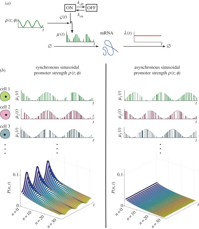
To illustrate this concept, we consider the modulated random telegraph (MRT) model, a combination of the RE model (3.1) and the RT model (3.9), i.e. the promoter strength is modulated by an upstream sinusoidal drive with random phase Φ, as in the RE model, yet the promoter switches stochastically between active/inactive states with rates k_on and k_off, as in the RT model. In this model, the transcription rate is correlated across cells through the entrainment to the upstream sinusoidal drive as a simple representation for, for example, circadian gene expression:

where m, ω > 0 are constants; Φ is the random phase across the cell population; and , with exponential waiting times, describes the stochastic promoter switching (figure 4a).

Figure 4.

(a) Modulated random telegraph model: each cell switches asynchronously between ‘ON’ and ‘OFF’ states, but the magnitude of the ‘ON’ transcription rate is modulated by the function ρ(t; ϕ), a sinusoid representing an upstream periodic process. The phase ϕ represents the cell-to-cell variability and leads to the varying degree of synchrony across the population. (b) Sample paths μ_i(t) and solution of the probability distribution P(n, t) of the MRT model for synchronous (left) and asynchronous (right) modulation. In the asynchronous case, the upstream drive has a random phase across the cells with distribution . (Online version in colour.)

The solution of this model follows from the RT probability density (3.10) conditioned on the random phase Φ, which prescribes the sample path of the promoter strength R. The resulting scaled Beta distribution

is then marginalized over the phase Φ to obtain the density of the effective drive. For instance, if the phases are normally distributed , we have (figure 4b)

As , the population becomes asynchronous in the promoter strength, as well as in the state transitions, and time dependence wanes (figure 4b).

4. Ensemble noise characteristics in time-varying populations

In the previous sections, we were concerned with the full time-dependent probability distribution P(n, t) for the mRNA copy number N. However, in many circumstances such detailed information is not required, and simpler characterizations based on ensemble averages (e.g. Fano factor, coefficient of variation) are of interest. Simple corollaries from the Poisson mixture expression (2.14) allow us to derive expressions for the ensemble moments and other noise characteristics, as shown below. We remark that, in this section, all the expectations are taken over the distribution describing the cell population.

4.1. Time-dependent ensemble moments over the distribution of cells

To quantify noise characteristics of gene expression in a population, the ensemble moments are often determined via the probability generating function [13,38,66] or by integrating the ME [21,40,67]. However, stationarity is usually assumed and the moments derived are not suitable for time-varying systems. Here we use corollaries of the Poisson mixture expression (2.14) to derive expressions for the ensemble moments for time-varying systems under upstream drives.

From (2.10), we have ; hence

are the Stirling numbers of the second kind [68]. The law of total probability then gives

4.1

or, equivalently,

Therefore, the ensemble moments of the mRNA copy number can be obtained in terms of the moments of the effective drive , and vice versa. For instance, it follows easily that ; ; and the skewness .

4.1.1. Decomposing the sources of noise

From equation (4.1), it follows that the variability of the mRNA count N_t can be rewritten as

4.2

i.e. it can be decomposed into a Poissonian (downstream) component and an upstream component linked to the variable X_t. Note, however, that our expressions (4.1) provide decompositions for all moments, and not only the mean and variance.

Expression (4.2) can be mapped onto the common decomposition into ‘intrinsic’ and ‘extrinsic’ components [48,49] if we note that, in our model, the ‘intrinsic’ components are the downstream processes of transcription and degradation, whose rates are affected by the ‘extrinsic’ variability due to upstream factors. Such upstream factors can be biologically diverse, and can be both intra- and extracellular. Therefore throughout this paper, we refer to ‘upstream/downstream’ processes instead of ‘intrinsic/extrinsic’ noise, to emphasize that upstream processes can reflect variability that is internal to the cell as well as cell-to-cell variability. For example, the asynchronous stochastic promoter switching described in §3.2 is an upstream process here, which in the literature might have been classed as ‘intrinsic’ (although in fact, asynchronicity implies an assumption about cell-to-cell variability). On the other hand, the modulated promoter switching in §3.3 includes both ‘intrinsic’ and ‘extrinsic’ sources of variability, as usually classed in the literature. In our framework, such processes are treated consistently as ‘upstream’ sources of variability.

4.1.2. Analysis of time-dependent moments

The relationship (4.1) between downstream and upstream moments together with the dynamical equation (2.13) enables us to solve for the time dependence of the moments of mRNA counts in terms of the moments of the drive:

4.3

4.4

where for simplicity we have assumed a constant degradation rate λ. (For the most general case with degradation rate L_t, see for example [45].) Therefore, the observed moments from the data can be used to infer the time-dependent moments of the (usually unobserved) upstream drives.

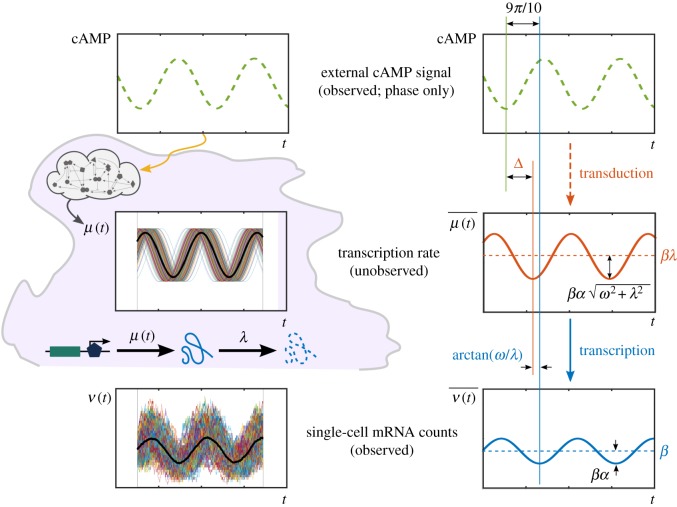
As a motivating example, we consider a recent experiment [29] measuring single-cell time courses of the expression of gene csaA in Dictyostelium discoideum when driven by a naturally oscillating extracellular cAMP signal. Corrigan and Chubb found that while individual single-cell time traces displayed no clear entrainment, with considerable heterogeneity both across time and across the population, there was a clear correlation between the external cAMP phase (measured by proxy through the cell speed) and the population-averaged, time-dependent level of csaA transcripts. This suggests that could generate precision in cell choices at the population level [29].

The experiment showed that the population-averaged mRNA expression was approximately sinusoidal. Hence, the data can be fitted to the function

4.5

Assuming a constant degradation rate λ, equations (2.13) and (4.3) show that the upstream transcription rate is also sinusoidal with the same frequency, yet with a modified amplitude and a phase shift (figure 5):

4.6

Figure 5.

Analysis of single-cell temporal transcription of a gene in response to an upstream oscillatory cAMP signal, motivated by recent experiments [29]. Individual single-cell time courses ν(t) of mRNA counts are highly variable with no clear entrainment to the driving signal, whereas the time-dependent ensemble average oscillates with the same frequency as the external drive. This is consistent with equations (4.5)–(4.6), which also show that the total phase lag is the resultant of the signal transduction and transcription lags. For a signal with period T = 5 min and a gene with degradation rate λ = 0.04 min⁻¹ [29], the transcription phase lag is , which corresponds to a delay of . Given a measured total mean lag of 9π/10, this implies that the signal transduction introduces a phase lag , equivalent to a delay of . (Online version in colour.)

This is similar to phase relationships in electrical and electronic circuits.

Consistent with equation (4.6), the cAMP phase and were measured experimentally to have the same frequency [29]. The experiments also showed that had a mean phase lag of 9π/10 (equivalent to a delay of ≈2.25 min) after the cAMP signal. Using the degradation rate λ = 0.04 min⁻¹ [69] for gene csaA, it follows that the transcriptional phase lag is arctan , and signal transduction introduces a phase lag , equivalent to a transduction delay . Hence our results can be used to adjudicate the time scales linked to cAMP signal transduction within the cell.

Our model also clarifies the effect of the degradation rate λ and frequency ω in the observed responses. Given the mRNA population average oscillating around a mean value β (4.5), the (unobserved) transcription rate oscillates with the same frequency ω around a value βλ and amplitude scaled by . The transcriptional phase lag is bounded between 0 (when ) and π/2 (when ). Hence, large degradation rates reduce the phase lag and the amplitude of the mRNA oscillations downstream (through the dimensionless factor ω/λ), and reduce the mean value of mRNA expression independently of ω.

A similar analysis for the correlation function can be achieved by solving equation (4.4) numerically for given data.

4.2. Time-dependent ensemble Fano factor: a measure of synchrony in the population

A commonly used measure of variability in the population is the ensemble Fano factor:

4.7

which is unity for the Poisson distribution. Its use has been popularized as a measure of the deviation from the stationary solution of the transcription of an unregulated gene with constant rates [70,71], which is Poisson; hence with .

For time-varying systems, however, the ensemble Fano factor conveys how the dynamic variability in single cells combines at the population level. Indeed, Fano(N_t) can be thought of as a measure of synchrony in the population at time t. For instance, it follows from equation (2.10) that the ensemble Fano factor for a population with perfectly synchronous drives is always equal to one, . Even if the upstream drive χ(t) changes in time, the population remains synchronous and has a Poisson distribution at all times. On the other hand, under the assumptions of our model, when Fano(N_t) varies in time, it reflects a change in the degree of synchrony between cells, as captured by the upstream drive X_t. From (4.1) it follows that

Hence, the greater the synchrony at time t, the closer Fano(N_t) is to unity, since the deviation from the Poisson distribution emanates from the ensemble Fano factor of the upstream drive X_t.

As an example, consider the Kuramoto promoter model (3.4)–(3.5) introduced in §3.1.2, where the cells in the population become more synchronized as the value of the coupling K is increased. Figure 6 shows simulation results for 100 cells with a range of couplings. The order parameter measures the phase coherence of the oscillators at time t; as r(t) approaches 1, the degree of synchrony increases. Using the Kuramoto numerics, we calculate the ensemble Fano factor Fano(N_t) for the transcription model. As seen in figure 6b,c, the more synchronous the system is, the closer the Fano factor is to the Poisson value, i.e. .

Figure 6 also illustrates the computational advantages of our method. The cost to approximate the time-varying ensemble moments is drastically reduced by using (4.1), because transcription and degradation events do not have to be simulated. The sample paths of the effective drive χ_i(t) were used to estimate the time-varying moments: and (shown in black). These correspond to the numerical simulation of ODEs, and are far more efficient than sampling from realizations ν_i(t) of the mRNA copy number.

5. Variability over time: stationarity and ergodicity

Our results up to now have not assumed stationarity; in general, the distribution (2.14) and moments (4.1) depend on time. If the cells in the population are uncorrelated and both M and L are stationary (i.e. their statistics do not change over time), then tends to a stationary density [45], and the full solution P(n, t) also tends to a stationary distribution P(n).

Under such assumptions leading to stationarity, any time dependence in P(n, t) only describes the ‘burn-in’ transient from an initial condition towards the attracting stationary distribution, as discussed in §2.1. Several examples of such transience have been studied in the literature, both in state switching models with constant rate parameters [16–18], and in a model with state-dependent rates [19], to describe how the distribution P(n, t) settles to stationarity when the process is started from an initial Kronecker delta distribution . Figure 7 and appendix A.2 analyse this transience explicitly for the RT model.

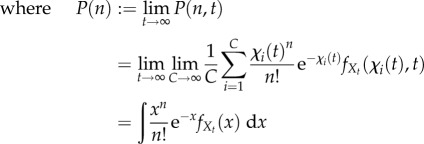
If, in addition to stationarity, we assume the cells to be indistinguishable, the population is ergodic. In this case, the distribution obtained from a single cell over a time T, as , is equivalent to the distribution obtained from a time snapshot at stationarity of a population of C cells, as , i.e.

5.1

5.2

5.3

Here, denotes time-averaging, and χ(t) in equation (5.3) is the sample path of the effective drive for a randomly chosen cell. Therefore, under the assumption of ergodicity, the averages computed over single-cell sample paths can be used to estimate the stationary distribution of the population.

5.1. Ergodic systems: stochastic versus deterministic drives

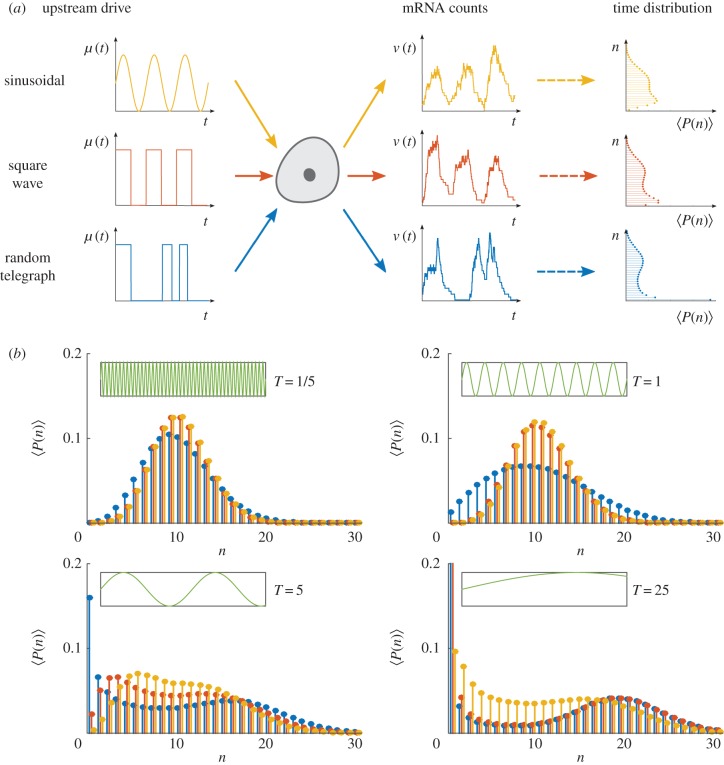
It has been suggested that stochastic and periodic drives lead to distinct properties in the noise characteristics within a cell population [49]. We investigate the effect of different temporal drives on the full distribution (2.14) under ergodicity using (5.1)–(5.3). Note that when χ(t) is periodic with period T, the limit in equation (5.3) is not required. In figure 8, we show the time-averaged distribution for a cell under three different upstream drives μ(t): (i) a continuous sinusoidal form; (ii) a discontinuous square wave form; (iii) a RT form, which can be thought of as the stochastic analogue of the square wave. In all cases, the drive with the same period, or expected period, T. For simplicity, we set .

Figure 8.

Ergodic transcription models under periodic and stochastic upstream drives. (a) We consider gene transcription under three drives : a sinusoidal wave with period T (yellow); a square wave with period T (red); a RT process with expected waiting time T/2 in each state (blue). For such ergodic systems, the distribution computed over time corresponds to the stationary distribution. (b) The distribution presents distinct features as the period T is varied. (Online version in colour.)

As the period T is varied, the similarity between the distributions under the three upstream drives varies considerably (figure 8). At small T, the distributions under sinusoidal and square wave forms are most similar; whereas at large T, the distributions under square wave and RT forms become most similar. In general, the distribution of the RT model has longer tails (i.e. n low and high) as a consequence of long (random) waiting times that allow the system to reach equilibrium in the active and inactive states, although this effect is less pronounced when the promoter switching is fast relative to the time scales of transcription and degradation (e.g. T = 1/5). On the other hand, as T grows, the square wave and RT drives are slow and the system is able to reach the equilibrium in both active and inactive states. Hence the probability distributions of the square wave and RT drives become similar, with a more prominent bimodality.

5.2. The temporal Fano factor: windows of stationarity in single-cell time-course data

The temporal Fano factor (TFF) is defined similarly to the ensemble version (4.7), but is calculated from the variance and mean of a single time series over a time window W ≔ (t₁, t₂):

5.4

In fact, this is the original definition of the Fano factor [72], which is used in signal processing to estimate statistical fluctuations of a count variable over a time window. Although N_t is not a count variable (it decreases with degradation events), the TFF can be used to detect windows of stationarity in single-cell time courses.

Figure 9a shows a single-cell sample path generated by the (leaky) RT model with constant degradation rate λ, and transcription rates μ₁> μ₀ > 0 for the active and inactive promoter states. The leaky RT model is equivalent to the standard RT model, and switches between two states with expectations μ₁/λ and μ₀/λ. In the time windows W between promoter switching, can be considered almost at stationarity and described by a Poisson distribution with parameter μ₀/λ (respectively, μ₁/λ) in the inactive (respectively, active) state. Hence across most of the sample path, except over the short transients W_trans when the system is switching between states, where (figure 9b).

Figure 9.

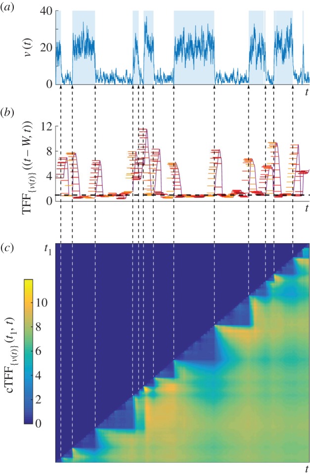
The temporal Fano factor. (a) A sample path of mRNA counts from the (leaky) RT model. The time periods when the gene is in the active state are shaded. (b) The temporal Fano factor (5.4), , computed over a time window W of fixed length indicated by the horizontal bars at each t. When W extends over a stationary section of the sample path, TFF is close to unity, corresponding to the Poisson distribution (black dashed line). (c) Heat map of the cTFF (5.5), , defined only for t ≥ t₁. Note the marked step pattern corresponding to the switching times, indicated by dashed lines as a guide to the eye. (Online version in colour.)

Alternatively, this information can be extracted robustly from the cumulative Fano factor (cTFF):

5.5

which is computed over a growing window from a fixed starting time t₁. The cTFF is a cumulative moving average giving an integrated description of how the stationary regimes are attained between switching events indicated by the step-like structure of the heat map in figure 9c.

6. Discussion

We have presented the solution of the ME for gene transcription with upstream dynamical variability in a setting that allows a unified treatment of a broad class of models, enabling quantitative biologists to go beyond stationary solutions when analysing noise sources in single-cell experiments. As a complementary approach to the explicit stochastic simulation of networks with many genes to account for the variability in data, our work uses a parsimonious transcription model of Poissonian type that includes explicitly the effect of dynamical and cell-to-cell upstream variability in the ME. We show that the solution to this gene transcription–degradation model can be expressed as a Poisson mixture form (2.14). This solution can be interpreted as the combination of an upstream component (dynamic or static; deterministic or stochastic) with a downstream Poissonian immigration–death process. Since only the upstream process is model-specific, different models are solved by obtaining the different mixing densities of the upstream process. This generic mathematical structure can describe both time-dependent snapshots across the population, as well as the dynamical variability over single-cell time courses in a coherent fashion.

The solution (2.14) can also be understood from the perspective of Gardiner and Chaturvedi's Poisson representation [36,37]. Originally, the Poisson representation was introduced as an ansatz for asymptotic expansions of stationary systems, and included only constant rate parameters. Hence the original Poisson representation ansatz has not been used widely for time-varying solutions [36]. In contrast, our time-dependent Poisson mixture (2.14) is obtained here as a solution to a non-stationary ME model, rather than backwards via basis expansions, and the mixing density has a physical interpretation in terms of single-cell sample paths relatable to data.

In this respect, our preparatory result (2.8) for the perfectly synchronous population can be thought of as an extension of the ‘Poisson representation’ to include time-varying rate parameters. Note also that this perfectly synchronous solution (2.8) corresponds to a particular case of the multigene solution obtained by Jahnke & Huisinga [34]. However, (2.8) does not yet encapsulate the cell-to-cell variability. It is the full Poisson mixture solution (2.14) that extends the scope of the time-varying ‘Poisson representation’ a step further, by allowing for stochastic rate parameters that can describe cell-to-cell variability as well as dynamic variability.

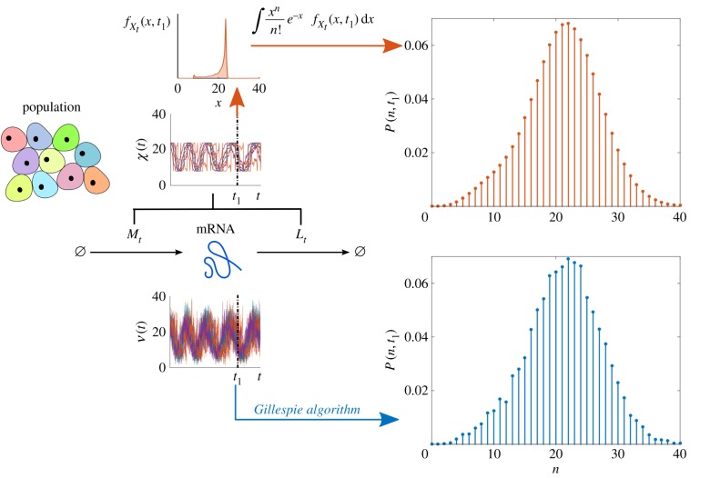
Our solution confers two broad advantages. The first is pragmatic: since X_t is a continuous random variable satisfying a linear random differential equation, we can draw upon the rich theory and analytical results for , even for non-stationary models, or we can use ODE and PDE solvers as further options to solve the differential equation for . If simulations are still necessary, sampling P(n, t|M, L) directly using stochastic simulation algorithms becomes computationally expensive, particularly if the upstream processes M and L are time-varying [73]. Instead, we can sample directly using the random differential equation (2.13), and then obtain the full distribution via numerical integration using (2.14). This approach leads to a significant reduction in computational cost, as shown in figure 10.

Figure 10.

Efficient sampling of the full distribution P(n, t) for transcription with upstream cellular drives. We consider upstream drives governed by the Kuramoto promoter model (3.4) for C = 10 000 coupled oscillatory cells. Sample paths of N are simulated directly with the Gillespie algorithm to approximate P(n, t) at time t₁ (bottom, blue). Alternatively, sample paths of X are used to estimate , which is then mixed by performing the numerical integration (2.14) to obtain P(n, t) (top, red). The latter sampling through X is more regular and far less costly: CPU time via N is ≈36000 s, whereas CPU time via X is ≈0.1 s. (Online version in colour.)

Our approach can also be used to analyse noise characteristics in conjunction with biological hypotheses. If measurements of additional cellular variables (e.g. cell cycle) are available, they can be incorporated as a source of variability for gene regulation to test biological hypotheses computationally against experimental data. Conversely, it is possible to discount the Poissonian component from observed data, so as to fit different promoter models to experimental data and perform model comparison [61]. Our discussion of a recent experiment of gene expression driven by cAMP signalling [29] exemplifies this approach.

The second advantage of our framework is conceptual. Through the natural decoupling of the solution into a discrete, Poisson component (downstream) and a continuous, mixing component (upstream), we derive time-dependent expressions for both ensemble and temporal moments, recasting the concept of ‘intrinsic’/’extrinsic’ noise for dynamic upstream cellular drives. Importantly, all upstream variability gets effectively imbricated through the upstream effective drive X, which can be interpreted in terms of a biochemical differential rate equation. This analysis clarifies how upstream fluctuations are combined to affect the probability distribution of the mRNA copy number, providing further intuition about the sources of noise and their temporal characteristics. Indeed, stripping the model down to its extrinsic component can provide us with additional understanding of its structure and time scales [61].

Finally, although we have concentrated here on the amenable analytical solutions that can be obtained for the single gene case, we remark that our solution could be extended to monomolecular multigene networks, by merging Jahnke & Huisinga's result [34] for synchronous networks with our mixture result for the asynchronous case. Such a generalization could be implemented computationally to reduce the cost of simulating stochastic networks. Such an extension will be the subject of future work. The solutions of higher-order reaction systems obtained through the Poisson representation ansatz could also be extended to include stochastic rates. This approach could lead to deeper understanding of models with and without feedback [74].

Appendix A. The ‘burn-in’ transient towards stationarity

In §2.1, it was stated that the contribution from the initial condition decreases exponentially for biophysically realistic degradation rates . As a result, the transcripts that were present at t = 0 are expected to degrade in finite time, and the long-term population is expected to be composed only of mRNA molecules that were transcribed since t = 0.

Let the initial condition be described by a random variable N₀ with a given probability distribution. It follows from equations (2.8)–(2.9) that

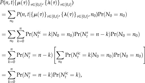where and are distributed according to equations (2.5)–(2.7), and is the mixture of the time-dependent binomial distribution (2.5) and the distribution of the initial condition N₀.

A.1. ‘Burn-in’ transience in the model with constant transcription and degradation

A.1.1. The decay towards stationarity

To understand the ‘burn-in’ period more explicitly, consider the simplest example of the gene transcription model (2.1) with constant transcription and degradation rates μ and λ, and assume that there are initially n₀ mRNA transcripts. Given that , the solution is given by

A 1

Hence as , the distribution will tend towards Poi(μ/λ), the stationary distribution of the population. This is a well-known result in the literature [37,75].

A.1.2. Starting at stationarity: the time-dependent and balance each other at all times

It is illustrative to consider the dynamics of this system when the initial condition is chosen to be the stationary distribution. In this case, the breakdown of N_t into the time-dependent components and will need to reproduce the stationary distribution at all times t > 0, with no ‘burn-in’ period.

To see this, let the initial distribution start at stationarity, i.e. and

The distribution of is still given by (A 1) and the contribution of is given by

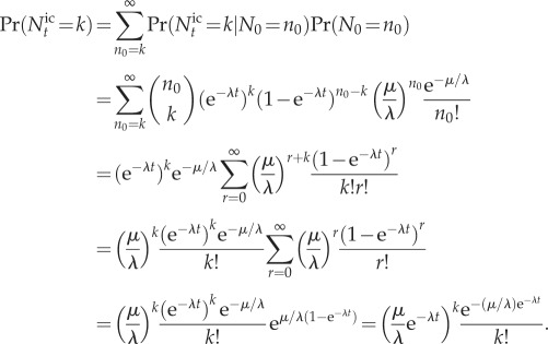In other words, , which cancels the contribution from . Therefore,

This example shows that and will combine to reproduce a stationary distribution at all times t > 0, when the system starts at stationarity so that there is no ‘burn-in’ transient.

A.1.3. Starting the system at

The same is true if the system is not stationary but we start the system at with any initial condition. Then, for t > 0, the system will be independent of the initial condition and will be described by .

Let us denote the state of the system for t > 0 by the attracting distribution P_*. Although , we wish to distinguish P_* from P_s because we only have equality of the two distributions when the system starts at . Here P_* can be thought of as an inherent property of the system, analogous to the stable point of a dynamical system that moves in time (sometimes called a chronotaxic system [76]).

If for all n₀ in equation (2.9), the contributions from and balance each other as they did in the case of stationarity with , and we would have (recall that the breakdown simply resolves the existing mRNA molecules into those that were present at t = 0, and those that were transcribed since t = 0). Thus we only observe an initial transient period if the initial distribution starts away from its attracting distribution at t = 0. In all other cases, the following mathematical formulations are equivalent: (i) assume that the system was initialized at and consider only or (ii) use the initial distribution for all n at t = 0, and consider .

In this work, we focus on the time dependence of P(n, t) induced through non-stationarity of the parameters, and/or synchronous behaviour of the cells within the population. Hence, unless otherwise stated, in this work we assume that the system was initialized at and that the distribution of is the attracting distribution P_*(n, t) for all t > 0, i.e. we neglect the contribution from .

A.2. ‘Burn-in’ transience in the random telegraph model

A time-dependent solution of the probability generating function for the RT model appeared in [16], although the explicit expression for P(n, t) was omitted. As discussed above, the RT model represents asynchronous and stationary behaviour, hence the time dependence appears only through convergence to the stationary distribution from the initial condition. We include the derivation here for completeness and to complement figure 7.

Consider the RT model depicted in figure 3a. Assuming that every cell is initialized in the inactive state with n₀ = 0 mRNA molecules, the probability generating function for the cell population is [16]

where , , and . Here ₁F₁(a, b; z) is the confluent hypergeometric function [63].

Using the general Leibniz rule for differentiation, and omitting other details, we obtain

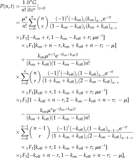where is Pochhammer's function [63].

As , . Hence as , , and we recover the known stationary solution:

Appendix B. The stationary solution for the refractory promoter model (three cyclic promoter states)

As explained in §3.2.2, the stationary solution of the 3-state cyclic model describing a refractory promoter is obtained by solving the following set of equations:

B 1

B 2

B 3

to obtain an expression for .

Note that the transition matrix [k_sr] containing the kinetic constants on the right-hand side of equations (B 1)–(B 3) is singular and hence λ = 0 is an eigenvalue. Furthermore, by Gershgorin's circle theorem the non-zero eigenvalues of [k_sr] have negative real parts, so a stationary solution always exists, i.e. the probabilities of being in state S_i evolve to an equilibrium state given by the eigenvector associated with the eigenvalue λ = 0. Note that must be normalized so that the elements sum to 1. It can easily be shown that

B 4

Now, integrating equations (B 1)–(B 3) and using equation (B 4) we obtain the boundary values and f_*(0) = 0. Also, summing equations (B 1)–(B 3) and integrating gives

B 5

where C is a constant. Equation (B 5) holds for all , so we can substitute in z = 0 or z = 1 and use the fact that f₁(1) = 0 and f₁(1) = 0, or f_*(0) = 0, to show that C = 0. Hence

B 6

so we need only solve equations (B 1)–(B 3) for f_*(z), the marginal probability density corresponding to the active state. Using (B 6) and substituting into (B 1)–(B 3), we then obtain the following equation for f_*(z):

B 7

Set , where c is a constant that we can choose, to transform (B 7) into

where and . From here, we set the last term on the right-hand side to zero by choosing c = k₁ or c = k₂. We can then divide through by z^{c + 1} to obtain an equation in the form of the hypergeometric equation [63]. For example, for c = k₁ we obtain

When none of , k₁ − k₂, or k_* are integers, we can write down the solution [63]

where C₁ and C₂ are constants of integration, ₂F₁[a, b; c; z] is the Gauss hypergeometric function [63] and

and

The solutions for the other cases are similar and are also given in [63]. Hence is given by

The same expression for f_*(z) is obtained if we choose c = k₂ instead, so finally we can write down the general solution for :

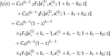B 8

Here, C₁ and C₂ are normalizing constants that ensure that the integral constraints

are satisfied. These constants are conveniently obtained from a Mellin transform identity (see [77, p. 152]):

where is the Gamma function [63]. Equation (B 8) is useful for comparisons with the 2-state RT model.

Data accessibility

No new data were collected in the course of this research.

Authors' contributions

J.D. carried out the calculations and simulations, participated in the design of the study and wrote the manuscript. M.B. conceived of the study, designed the study, coordinated the study and wrote the manuscript. Both authors gave their final approval for publication.

Competing interests

The authors declare no competing interests.

Funding

J.D. was funded by an EPSRC PhD studentship. M.B. acknowledges funding from the EPSRC through grant nos. EP/I017267/1 and EP/N014529/1.

References

- 1.Levine M, Tjian R. 2003. Transcription regulation and animal diversity. Nature 424, 147–151. ( 10.1038/nature01763) [DOI] [PubMed] [Google Scholar]
- 2.Raj A, van Oudenaarden A. 2008. Nature, nurture, or chance: stochastic gene expression and its consequences. Cell 135, 216–226. ( 10.1016/j.cell.2008.09.050) [DOI] [PMC free article] [PubMed] [Google Scholar]
- 3.Owens NDL, Blitz IL, Lane MA, Patrushev I, Overton JD, Gilchrist MJ, Cho KWY, Khoka MK. 2016. Measuring absolute RNA copy numbers at high temporal resolution reveals transcriptome kinetics in development. Cell Rep. 14, 632–647. ( 10.1016/j.celrep.2015.12.050) [DOI] [PMC free article] [PubMed] [Google Scholar]
- 4.Singer ZS, Yong J, Tischler J, Hackett JA, Altinok A, Surani MA, Cai L, Elowitz MB. 2014. Dynamic heterogeneity and DNA methylation in embryonic stem cells. Mol. Cell 55, 319–331. ( 10.1016/j.molcel.2014.06.029) [DOI] [PMC free article] [PubMed] [Google Scholar]
- 5.Maamar H, Raj A, Dubnau D. 2007. Noise in gene expression determines cell fate in Bacillus subtilis. Science 317, 526–529. ( 10.1126/science.1140818) [DOI] [PMC free article] [PubMed] [Google Scholar]
- 6.Chang HH, Hemberg M, Barahona M, Ingber DE, Huang S. 2008. Transcriptome-wide noise controls lineage choice in mammalian progenitor cells. Nature 453, 544–547. ( 10.1038/nature06965) [DOI] [PMC free article] [PubMed] [Google Scholar]
- 7.Balázsi G, van Oudenaarden A, Collins JJ. 2011. Cellular decision making and biological noise: from microbes to mammals. Cell 144, 910–925. ( 10.1016/j.cell.2011.01.030) [DOI] [PMC free article] [PubMed] [Google Scholar]
- 8.Garcia-Ojalvo J, Arias AM. 2012. Towards a statistical mechanics of cell fate decisions. Curr. Opin. Genet. Dev. 22, 619–626. ( 10.1016/j.gde.2012.10.004) [DOI] [PubMed] [Google Scholar]
- 9.Wolf L, Silander OK, van Nimwegen E. 2015. Expression noise facilitates the evolution of gene regulation. eLife 4, e05856 ( 10.7554/eLife.05856) [DOI] [PMC free article] [PubMed] [Google Scholar]
- 10.Wilkinson DJ. 2009. Stochastic modelling for quantitative description of heterogeneous biological systems. Nat. Rev. Genet. 10, 122–133. ( 10.1038/nrg2509) [DOI] [PubMed] [Google Scholar]
- 11.Hornos JEM, Schultz D, Innocentini GCP, Wang J, Walczak AM, Onuchic JN, Wolynes PG. 2005. Self-regulating gene: an exact solution. Phys. Rev. E 72, 051907 ( 10.1103/PhysRevE.72.051907) [DOI] [PubMed] [Google Scholar]
- 12.Visco P, Allen RJ, Evans MR. 2008. Exact solution of a model DNA-inversion genetic switch with orientational control. Phys. Rev. Lett. 101, 118104 ( 10.1103/PhysRevLett.101.118104) [DOI] [PubMed] [Google Scholar]
- 13.Zhang J, Chen L, Zhou T. 2012. Analytical distribution and tunability of noise in a model of promoter progress. Biophys. J. 102, 1247–1257. ( 10.1016/j.bpj.2012.02.001) [DOI] [PMC free article] [PubMed] [Google Scholar]
- 14.Pendar H, Platini T, Kulkarni RV. 2013. Exact protein distributions for stochastic models of gene expression using partitioning of Poisson processes. Phys. Rev. E 87, 042720 ( 10.1103/PhysRevE.87.042720) [DOI] [PubMed] [Google Scholar]
- 15.Kumar N, Platini T, Kulkarni RV. 2014. Exact distributions for stochastic gene expression models with bursting and feedback. Phys. Rev. Lett. 113, 268105 ( 10.1103/PhysRevLett.113.268105) [DOI] [PubMed] [Google Scholar]
- 16.Iyer-Biswas S, Hayot F, Jayaprakash C. 2009. Stochasticity of gene products from transcriptional pulsing. Phys. Rev. E 79, 031911 ( 10.1103/PhysRevE.79.031911) [DOI] [PubMed] [Google Scholar]
- 17.Shahrezaei V, Swain PS. 2008. Analytical distributions for stochastic gene expression. Proc. Natl Acad. Sci. USA 105, 17 256–17 261. ( 10.1073/pnas.0803850105) [DOI] [PMC free article] [PubMed] [Google Scholar]
- 18.Vandecan Y, Blossey R. 2013. Self-regulatory gene: an exact solution for the gene gate model. Phys. Rev. E 87, 042705 ( 10.1103/PhysRevE.87.042705) [DOI] [PubMed] [Google Scholar]
- 19.Smith S, Shahrezaei V. 2015. General transient solution of the one-step master equation in one dimension. Phys. Rev. E 91, 062119 ( 10.1103/PhysRevE.91.062119) [DOI] [PubMed] [Google Scholar]
- 20.Paulsson J. 2005. Models of stochastic gene expression. Phys. Life Rev. 2, 157–175. ( 10.1016/j.plrev.2005.03.003) [DOI] [Google Scholar]
- 21.Sánchez A, Golding I. 2013. Genetic determinants and cellular constraints in noisy gene expression. Science 342, 1188–1193. ( 10.1126/science.1242975) [DOI] [PMC free article] [PubMed] [Google Scholar]
- 22.Zeron ES, Santillán M. 2011. Numerical solution of the chemical master equation: uniqueness and stability of the stationary distribution for chemical networks, and mRNA bursting in a gene network with negative feedback regulation. Methods Enzymol. 487, 147–169. ( 10.1016/B978-0-12-381270-4.00006-8) [DOI] [PubMed] [Google Scholar]
- 23.Crosetto N, Bienko M, van Oudenaarden A. 2015. Spatially resolved transcriptomics and beyond. Nat. Rev. Genet. 16, 57–66. ( 10.1038/nrg3832) [DOI] [PubMed] [Google Scholar]
- 24.Park HY, Lim H, Yoon YJ, Follenzi A, Nwokafor C, Lopez-Jones M, Meng X, Singer RH. 2014. Visualization of dynamics of single endogenous mRNA labeled in live mouse. Science 343, 422–424. ( 10.1126/science.1239200) [DOI] [PMC free article] [PubMed] [Google Scholar]
- 25.Young JW, Locke JCW, Altinok A, Rosenfeld N, Bacarian T, Swain PS, Mjolsness E, Elowitz MB. 2012. Measuring single-cell gene expression dynamics in bacteria using fluorescence time-lapse microscopy. Nat. Protocols 7, 80–88. ( 10.1038/nprot.2011.432) [DOI] [PMC free article] [PubMed] [Google Scholar]
- 26.Junker JP, Van Oudenaarden A. 2014. Every cell is special: genome-wide studies add a new dimension to single-cell biology. Cell 157, 8–11. ( 10.1016/j.cell.2014.02.010) [DOI] [PubMed] [Google Scholar]
- 27.Mihalcescu I, Hsing W, Leibler S. 2004. Resilient circadian oscillator revealed in individual cyanobacteria. Nature 430, 81–85. ( 10.1038/nature02533) [DOI] [PubMed] [Google Scholar]
- 28.Bieler J, Cannavo R, Gustafson K, Gobet C, Gatfield D, Naef F. 2014. Robust synchronization of coupled circadian and cell cycle oscillators in single mammalian cells. Mol. Syst. Biol. 10, 739 ( 10.15252/msb.20145218) [DOI] [PMC free article] [PubMed] [Google Scholar]
- 29.Corrigan AM, Chubb JR. 2014. Regulation of transcriptional bursting by a naturally oscillating signal. Curr. Biol. 24, 205–211. ( 10.1016/j.cub.2013.12.011) [DOI] [PMC free article] [PubMed] [Google Scholar]
- 30.Molina N, Suter DM, Cannavoa R, Zoller B, Gotic I, Naef F. 2013. Stimulus-induced modulation of transcriptional bursting in a single mammalian gene. Proc. Natl Acad. Sci. USA 110, 20 563–20 568. ( 10.1073/pnas.1312310110) [DOI] [PMC free article] [PubMed] [Google Scholar]
- 31.Konermann S, et al. 2013. Optical control of mammalian endogenous transcription and epigenetic states. Nature 500, 472–476. ( 10.1038/nature12466) [DOI] [PMC free article] [PubMed] [Google Scholar]
- 32.Zechner C, Koeppl H. 2014. Uncoupled analysis of stochastic reaction networks in fluctuating environments. PLoS Comput. Biol. 10, e1003942 ( 10.1371/journal.pcbi.1003942) [DOI] [PMC free article] [PubMed] [Google Scholar]
- 33.Almquist J, Bendrioua L, Aliels CB, Goksör M, Hohmann S, Jirstrand M. 2015. A nonlinear mixed effects approach for modeling the cell-to-cell variability of Mig1 dynamics in yeast. PLoS ONE 10, e0124050 ( 10.1371/journal.pone.0124050) [DOI] [PMC free article] [PubMed] [Google Scholar]
- 34.Jahnke T, Huisinga W. 2007. Solving the chemical master equation for monomolecular reaction systems analytically. J. Math. Biol. 54, 1–26. ( 10.1007/s00285-006-0034-x) [DOI] [PubMed] [Google Scholar]
- 35.Eick SG, Massey WA, Whitt W. 1993. Physics of the Mt/G/∞ queue. Operat. Res. 41, 731–742. ( 10.1287/opre.41.4.731) [DOI] [Google Scholar]
- 36.Gardiner CW, Chaturvedi S. 1977. The Poisson representation. I. A new technique for chemical master equations. J. Stat. Phys. 17, 429–468. ( 10.1007/BF01014349) [DOI] [Google Scholar]
- 37.Gardiner CW. 1985. Handbook of stochastic methods, 2nd edn Berlin, Germany: Springer. [Google Scholar]
- 38.Peccoud J, Ycart B. 1995. Markovian modeling of gene-product synthesis. Theoret. Popul. Biol. 48, 222–234. ( 10.1006/tpbi.1995.1027) [DOI] [Google Scholar]
- 39.Raj A, Peskin CS, Tranchina D, Vargas DY, Tyagi S. 2006. Stochastic mRNA synthesis in mammalian cells. PLoS Biol. 4, 1707–1719. ( 10.1371/journal.pbio.0040309) [DOI] [PMC free article] [PubMed] [Google Scholar]
- 40.Sánchez A, Garcia HG, Jones D, Phillips R, Kondev J. 2008. Effect of promoter architecture on the cell-to-cell variability in gene expression. PLoS Comput. Biol. 105, 5081–5086. [DOI] [PMC free article] [PubMed] [Google Scholar]
- 41.Senecal A, Munsky B, Proux F, Ly N, Braye FE, Zimmer C, Mueller F, Darzacq X. 2014. Transcription factors modulate c-Fos transcriptional bursts. Cell Rep. 8, 75–83. ( 10.1016/j.celrep.2014.05.053) [DOI] [PMC free article] [PubMed] [Google Scholar]
- 42.Zoller B, Nicolas D, Molina N, Naef F. 2015. Structure of silent transcription intervals and noise characteristics of mammalian genes. Mol. Syst. Biol. 11, 823 ( 10.15252/msb.20156257) [DOI] [PMC free article] [PubMed] [Google Scholar]
- 43.Todorovic P. 1992. An introduction to stochastic processes and their applications. Berlin, Germany: Springer. [Google Scholar]
- 44.van Kampen NG. 1992. Stochastic processes in physics and chemistry, 2nd edn Amsterdam, The Netherlands: Elsevier. [Google Scholar]
- 45.Soong TT. 1973. Random differential equations in science and engineering, vol. 103. Mathematics in Science and Engineering New York, NY: Academic Press. [Google Scholar]
- 46.Pawula R. 1967. Generalizations and extensions of the Fokker-Planck-Kolmogorov equations. IEEE Trans. Inform. Theory 13, 33–41. ( 10.1109/TIT.1967.1053955) [DOI] [Google Scholar]
- 47.Elowitz MB, Levine AJ, Siggia ED, Swain PS. 2002. Stochastic gene expression in a single cell. Science 297, 1183–1186. ( 10.1126/science.1070919) [DOI] [PubMed] [Google Scholar]
- 48.Swain PS, Elowitz MB. 2002. Intrinsic and extrinsic contributions to stochasticity in gene expression. Proc. Natl Acad. Sci. USA 99, 12 795–12 800. ( 10.1073/pnas.162041399) [DOI] [PMC free article] [PubMed] [Google Scholar]
- 49.Hilfinger A, Paulsson J. 2011. Separating intrinsic from extrinsic fluctuations in dynamic biological systems. Proc. Natl Acad. Sci. USA 108, 12 167–12 172. ( 10.1073/pnas.1018832108) [DOI] [PMC free article] [PubMed] [Google Scholar]
- 50.Bowsher CG, Swain PS. 2012. Identifying sources of variation and the flow of information in biochemical networks. Proc. Natl Acad. Sci. USA 109, E1320–E1328. ( 10.1073/pnas.1119407109) [DOI] [PMC free article] [PubMed] [Google Scholar]
- 51.Lück S, Thurley K, Thaben PF, Westermark PO. 2014. Rhythmic degradation explains and unifies circadian transcriptome and proteome data. Cell Rep. 9, 741–751. ( 10.1016/j.celrep.2014.09.021) [DOI] [PubMed] [Google Scholar]
- 52.Kuramoto Y. 1975. Self-entrainment of a population of coupled non-linear oscillators. In Int. Symp. on Mathematical Problems in Theoretical Physics (ed. H Araki). Lecture Notes in Physics, vol. 39, pp. 420–422. Berlin, Germany: Springer ( 10.1007/BFb0013365) [DOI]
- 53.Strogatz SH. 2000. From Kuramoto to Crawford: exploring the onset of synchronization in populations of coupled oscillators. Phys. D: Nonlinear Phenomena 143, 1–20. ( 10.1016/S0167-2789(00)00094-4) [DOI] [Google Scholar]
- 54.Jadbabaie A, Motee N, Barahona M.2004. On the stability of the Kuramoto model of coupled nonlinear oscillators. In IEEE American Control Conf., Boston, MA, USA, 30 June–2 July 2004, vol. 5, pp. 4296–4301.
- 55.Garcia-Ojalvo J, Elowitz MB, Strogatz SH. 2004. Modeling a synthetic multicellular clock: repressilators coupled by quorum sensing. Proc. Natl Acad. Sci. USA 101, 10 955–10 960. ( 10.1073/pnas.0307095101) [DOI] [PMC free article] [PubMed] [Google Scholar]
- 56.Taylor AF, Tinsley MR, Wang F, Huang Z, Showalter K. 2009. Dynamical quorum sensing and synchronization in large populations of chemical oscillators. Science 323, 614–617. ( 10.1126/science.1166253) [DOI] [PubMed] [Google Scholar]
- 57.Murray PJ, Maini PK, Baker RE. 2011. The clock and wavefront model revisited. J. Theoret. Biol. 283, 227–238. ( 10.1016/j.jtbi.2011.05.004) [DOI] [PubMed] [Google Scholar]
- 58.Uriu K, Ares S, Oates AC, Morelli LG. 2012. Optimal cellular mobility for synchronization arising from the gradual recovery of intercellular interactions. Phys. Biol. 9, 036006 ( 10.1088/1478-3975/9/3/036006) [DOI] [PubMed] [Google Scholar]
- 59.Pawula R. 1970. The transition probability density function of the low-pass filtered random telegraph signal. Int. J. Control 12, 25–32. ( 10.1080/00207177008931818) [DOI] [Google Scholar]
- 60.Ko M. 1991. A stochastic model for gene induction. J. Theoret. Biol. 153, 181–194. ( 10.1016/S0022-5193(05)80421-7) [DOI] [PubMed] [Google Scholar]
- 61.Dattani J. 2016. Exact solutions of master equations for the analysis of gene transcription models. PhD thesis, Imperial College London, UK.
- 62.Smiley MW, Proulx SR. 2010. Gene expression dynamics in randomly varying environments. J. Math. Biol. 61, 231–251. ( 10.1007/s00285-009-0298-z) [DOI] [PubMed] [Google Scholar]
- 63.Abramowitz M, Stegun IA. 1964. Handbook of mathematical functions. New York, NY: Dover. [Google Scholar]
- 64.Suter DM, Molina N, Gatfield D, Schneider K, Schibler U, Naef F. 2011. Mammalian genes are transcribed with widely different bursting kinetics. Science 332, 472–474. ( 10.1126/science.1198817) [DOI] [PubMed] [Google Scholar]
- 65.Hasenauer J, Wolf V, Kazeroonian A, Theis FJ. 2014. Method of conditional moments (MCM) for the chemical master equation. J. Math. Biol. 69, 687–735. ( 10.1007/s00285-013-0711-5) [DOI] [PubMed] [Google Scholar]
- 66.Paszek P. 2007. Modeling stochasticity in gene regulation: characterization in the terms of the underlying distribution function. Bull. Math. Biol. 69, 1567–1601. ( 10.1007/s11538-006-9176-7) [DOI] [PubMed] [Google Scholar]
- 67.Sánchez A, Kondev J. 2008. Transcriptional control of noise in gene expression. Proc. Natl Acad. Sci. USA 105, 5081–5086. ( 10.1073/pnas.0707904105) [DOI] [PMC free article] [PubMed] [Google Scholar]
- 68.Riordan J. 1937. Moment recurrence relations for binomial, Poisson and hypergeometric frequency distributions. Ann. Math. Stat. 8, 103–111. ( 10.1214/aoms/1177732430) [DOI] [Google Scholar]
- 69.Muramoto T, Cannona D, Gierliński M, Corrigan A, Barton GJ, Chubb JR. 2012. Live imaging of nascent RNA dynamics reveals distinct types of transcriptional pulse regulation. Proc. Natl Acad. Sci. USA 109, 7350–7355. ( 10.1073/pnas.1117603109) [DOI] [PMC free article] [PubMed] [Google Scholar]
- 70.Thattai M, van Oudenaarden A. 2001. Intrinsic noise in gene regulatory networks. Proc. Natl Acad. Sci. USA, 98, 8614–8619. ( 10.1073/pnas.151588598) [DOI] [PMC free article] [PubMed] [Google Scholar]
- 71.Raj A, Van Oudenaarden A. 2009. Single-molecule approaches to stochastic gene expression. Annu. Rev. Biophys. 38, 255–270. ( 10.1146/annurev.biophys.37.032807.125928) [DOI] [PMC free article] [PubMed] [Google Scholar]
- 72.Fano U. 1947. Ionization yield of radiations. II. The fluctuations of the number of ions. Phys. Rev. 72, 26–29. ( 10.1103/PhysRev.72.26) [DOI] [Google Scholar]
- 73.Shahrezaei V, Olivier JF, Swain PS. 2008. Colored extrinsic fluctuations and stochastic gene expression. Mol. Syst. Biol. 4, 196 ( 10.1038/msb.2008.31) [DOI] [PMC free article] [PubMed] [Google Scholar]
- 74.Iyer-Biswas S, Jayaprakash C. 2014. Mixed Poisson distributions in exact solutions of stochastic autoregulation models. Phys. Rev. E 90, 052712 ( 10.1103/PhysRevE.90.052712) [DOI] [PubMed] [Google Scholar]
- 75.Brémaud P. 2001. Markov chains, Gibbs fields, Monte Carlo simulation and queues. Berlin, Germany: Springer. [Google Scholar]
- 76.Suprunenko YF, Clemson PT, Stefanovska A. 2013. Chronotaxic systems: a new class of selfsustained nonautonomous oscillators. Phys. Rev. Lett. 111, 024101 ( 10.1103/PhysRevLett.111.024101) [DOI] [PubMed] [Google Scholar]
- 77.Slater LJ. 1966. Generalized hypergeometric functions. Cambridge, UK: Cambridge University Press. [Google Scholar]
Associated Data
This section collects any data citations, data availability statements, or supplementary materials included in this article.
Data Availability Statement