Nonlinear dynamics as an engine of computation

Abstract

Control of chaos teaches that control theory can tame the complex, random-like behaviour of chaotic systems. This alliance between control methods and physics—cybernetical physics—opens the door to many applications, including dynamics-based computing. In this article, we introduce nonlinear dynamics and its rich, sometimes chaotic behaviour as an engine of computation. We review our work that has demonstrated how to compute using nonlinear dynamics. Furthermore, we investigate the interrelationship between invariant measures of a dynamical system and its computing power to strengthen the bridge between physics and computation.

This article is part of the themed issue ‘Horizons of cybernetical physics’.

1. Introduction

Linearity is usually praised as a positive feature and property in many disciplines, and even in common language. Linearity is considered synonymous to, and associated with, ease of use and predictability. Abundant tools and techniques to solve and analyse linear systems exist. System designers and engineers favour linearity because linearity keeps system behaviour simple, predictable and easy to manage and alter. System analysts prefer linearity because they can describe, model and solve linear systems efficiently.

Unlike linearity, nonlinearity is sometimes considered as a negative feature, as a hurdle, as an uncertainty and with a lack of ease. Designing nonlinear systems can be harder because nonlinear interactions or behaviours in the system must be taken into account, and there is no generic tool to analyse and solve nonlinear systems.

Simply put, nonlinearity refers to a relationship that cannot be modelled or explained as a linear algebraic or differential combination of input or state variables. The consequences of this lack of linearity are fundamental and substantial, and nonlinear systems differ completely from linear systems. The behaviour of a nonlinear system can be sensitive to the parameters of the systems and the initial conditions of the system. More specifically, by changing a nonlinear system's parameters, the behaviour of the system can change qualitatively, as well as quantitatively. For example, upon changing a bifurcation parameter, the system can switch between different periodic states, and eventually it can reach full chaos. Or a nonlinear system can be globally stable, but locally unstable, meaning that, despite having an attractor, it can be extremely sensitive to initial conditions. A chaotic system contains an infinite number of different periodic orbits, which are dense in the state space of the system.

These arguments might mislead us to believing that nonlinearity is a feature to be avoided. But we live in a nonlinear world. Nature is nonlinear, and its nonlinearity plays a fundamental role in its performance and functionality. The flexibility of natural and living systems and their ability to adapt to and cope with different conditions is believed to originate from nonlinearity [1]. Even human-made systems such as transistors, vacuum tubes and triodes are nonlinear in nature, although their nonlinearity has not been fully used in engineered systems.

In a nutshell, a nonlinear system can be considered to be a complex library of different behaviours. Starting in the 1990s, advances in control theory and dynamical systems theory enabled us to hack into these nonlinear complex systems and use their inner complexity better. Ditto & Pecora [2] published one of the earliest reports on the applications of chaos theory that were enabled by the introduction of control of chaos. Andrievskii & Fradkov [3,4] provide an extensive list of different categories of chaos control methods and applications. And we discuss [5] how complex nonlinear dynamics can be tailored and used to perform different types of computation. With the help of such control and dynamical systems theory techniques, also called cybernetics, the chaos was tamed and complex systems were revealed to be vast libraries of diverse and accessible behaviours. This application of cybernetical methods to nonlinear complex systems in order to transform, control, synchronize or use their dynamics is called cybernetical physics [6].

Nonlinear dynamics-based computing was one of the applications that emerged as a consequence of chaos control and the taming of chaos. The driving motivation behind nonlinear dynamics-based computing, or chaos computing for short, was the question: what if chaotic systems are actually performing some form of computation? And how can we tame and domesticate these chaotic systems to perform computation for us [7]? In this paper, and the previous literature related to this paper, the terms chaos computing, dynamics-based computing and nonlinear dynamics-based computing are used interchangeably, and they all refer to the same concept, namely the utilization of the inherent, complex dynamics of nonlinear dynamical systems to perform computation. The main advantage of nonlinear dynamics-based computing is that each intrinsic behaviour of the dynamical system can represent a different type of computation, and a nonlinear dynamical system contains many different behaviours, each of which can be selected. As a result, a nonlinear dynamical system can embody different types of computations, and one can dynamically programme the system to perform different types of computations.

A simple Turing machine can also be programmed to implement different types of computation. However, in nonlinear dynamics-based computing all the different types of computation coexist in the dynamics of the same system, and are embodied by the same system, whereas the Turing machine must be programmed to ‘simulate’ these different types of computation one by one. This is the difference between actual implementation and simulation. The difference becomes even more vivid when we consider the implementation of nonlinear dynamics-based computing [8], where we show how even a simple ideal transistor circuit contains an infinite number of different functions.

It is important to note that a conventional computer system is a nonlinear dynamical system by itself, and the circuits within this system are all nonlinear dynamical systems. However, we do not call conventional computers nonlinear dynamics-based computing systems because the nonlinearity and its complex dynamics are not fully and directly used in the computation. Analogously, despite conventional computers being all composed of microscopic particles governed by quantum mechanics, conventional computer systems are not called quantum computers because the quantum mechanics is not directly used in the computation. In nonlinear dynamics-based computing, the computing is carved from nonlinear dynamics, and nonlinear dynamics is the engine of the computation. It is the mechanism that maps the inputs to the outputs, and it is nonlinear dynamics that is used to programme the nonlinear dynamics-based computer to perform different computation.

In §2, we review nonlinear dynamics-based computing. In §3, we connect nonlinear dynamics and invariant measures to inherent computational powers using the computing exponent. The paper is concluded in §4.

2. Dynamics-based computing

Many abstract computing machines, such as a Turing machine or cellular automata, have been regarded and studied as discontinuous dynamical systems or as symbolic dynamical systems [9–11]. The complexity of a general dynamical system has been characterized by its computing power [12], and the dynamical properties of a dynamical system have been linked to its computational properties [13].

In the majority of such approaches, the focus has been on traditional abstract computing models with less work on physical circuits and systems, how the dynamics of physical systems could perform computation, and how to use such physical systems as actual computer systems. We introduced a practical dynamics-based approach for computation where the intrinsic dynamics of a physical system can be used to perform combinational logic operations [5,7]. In such an approach, the intrinsic dynamics of a physical system is observed as a function that maps the initial condition of the dynamical system to future states. Signals in a majority of real-world systems are analogue, meaning that the dynamical variables of a real-world dynamical system are continuous in value. To implement digital functions, we used encoder and decoder maps that encode incoming binary data as an analogue initial condition and decode a binary output from the analogue output.

Because a nonlinear system contains many different behaviours, and its dynamics—the mapping between inputs and outputs—can be dynamically controlled and altered using different cybernetical methods, nonlinear dynamics can provide us with a universal computing system that can be programmed to implement different functions. We call our dynamics-based reconfigurable computing system ‘universal’ in the sense that it can be programmed to implement many functions.

A block diagram for our nonlinear dynamics-based computing model is depicted in figure 1. Binary data inputs, denoted by d, are encoded as an initial condition of the nonlinear system. And an output, O, is decoded from the final state of the nonlinear system. Two control inputs, c and p, programme the nonlinear system to implement different functions. Input p changes the bifurcation parameter of the nonlinear system and alters the dynamics of the system, and therefore changes the mapping between inputs and outputs and the type of function the nonlinear system builds. Input c perturbs the nonlinear system and therefore changes the dynamical evolution of the system, especially when the nonlinear system is in a chaotic regime. As a result, c can be used to programme the dynamical system to also implement different functions. Furthermore, when the dynamics is chaotic, or periodic with a long periodicity, the observed state of the dynamical system x_n varies with evolution time n, and as a result different outputs and different types of functions can be obtained for different evolution time n. We have previously discussed techniques to programme a nonlinear dynamical system to implement different functions in detail [5].

Figure 1.

Block diagram for a nonlinear dynamics-based computing system.

When the nonlinear dynamical system is in a chaotic regime, noise can, and does, change the future states of the system. However, in this method, the evolution time is set to be short enough that noise does not have enough time to evolve, great enough to smear the future state of the system and change the output, but long enough so that the relatively large control inputs c can change the future state of the system and programme the nonlinear system to implement a different function. Kia et al. [14,15] analyse the effects of noise on chaos computing and discuss how dynamically coupling identical nonlinear systems, performing reconfigurable computing, can systematically reduce the noise sensitivity of this type of computation and improve its robustness to noise [16].

The advantage of this nonlinear dynamics-based approach for computing is twofold. Firstly, different types of functions coexist within a nonlinear dynamical system. In other words, one nonlinear circuit or system can implement different types of functions and computations. This is a very important capability given that Moore's law is approaching physical limits.

Moore's law is an observation and prediction that the number of transistors on an integrated chip doubles every 24 months, and this exponential increase of transistors fulfils market needs and demands for computers with exponentially increasing performance [17]. But today this trend is slowing down because the size of devices is reaching atomic levels [18]. Furthermore, the power consumption of transistors over successive generations has not continued to scale with decreasing transistor size. Consequently, power consumption has become another limiting factor in determining the maximum transistor density that can be effectively used on many integrated circuits [18]. As a result, we cannot simply increase the performance of computers by packing more and more devices in an integrated circuit any more. One of the major alternative methods that semiconductor companies and academia have taken is to enhance and improve the utilization of currently available transistors rather than trying to pack more transistors into the chip. In other words, the main idea of such approaches is to get more out of few transistors, such as by using enhanced computer architecture [18] or by improving the bit handling capacity of devices [19].

Nonlinear dynamics-based computing introduces a new solution. In this dynamics-based approach, the computation is performed at the dynamical level, where many different types of computation coexist, with special thanks to the complex dynamics of nonlinear systems. Furthermore, very simple transistor circuits can have very complex nonlinear dynamics. Therefore, by utilizing dynamical systems for computation, we can perform many different types of computation using very simple transistor circuits. Recently [8], we showed that an ideal nonlinear circuit contains an infinite number of different functions. This opens the door for better utilization of transistors to gain more computation out of a fixed number of transistors by reconfiguring the same circuit to implement multiple different types of computation, rather than needing multiple different circuits for different types of computation.

The second advantage of the nonlinear dynamics-based approach is that programming and reconfiguring a nonlinear dynamical system to implement a different type of computation does not require any halting of the system or a separate programming phase. Rather, the programming inputs are fed to the system along with the data inputs at the same time, and processing and programming happen in the same clock cycle. This enables us to design processing units that at each clock cycle, depending on the needs or the specific instruction that the unit has to execute, the unit can be instantaneously and dynamically programmed to implement the new type of computation. The main reason is that different types of computations coexist within the same system, and we are just picking them up from the system rather than loading a new function to the system—the scenario that happens in programmable gate arrays, or in short FPGAs.

We have recently designed, fabricated, and tested and verified an integrated circuit for nonlinear dynamics-based computing. The fabricated circuit can be dynamically programmed to implement all two-input, one-output digital functions [20]. In this paper, we do not discuss the details of hardware design for such a reconfigurable system. Such topics are the focus of our other papers. Instead, here we focus on an abstract ideal, mathematical model for how such a nonlinear dynamics-based reconfigurable system works, and how the amount of computation such a nonlinear dynamics-based computing system can perform is connected to its physics.

3. Computing measures complexity

A dynamical system maps its initial conditions to its future states like a function maps inputs to outputs. In this way, linear dynamical systems implement simple linear functions, while nonlinear dynamical systems implement complex, nonlinear functions. Dynamics is intrinsic computation.

Understanding and measuring complexity are important problems. Complexity has different aspects and different measures have been introduced to quantify them [21]. Lloyd [22] has even estimated the computational capacity of the Universe. In this section, we consider dynamical systems, which naturally instantiate functions, and introduce a metric, the computing exponent, to measure the amount of computation they can perform.

(a). Three metrics

The computing exponent is related to two other important complexity measures, the Lyapunov exponent and the topological entropy. For simplicity, we consider one-dimensional maps x_n+1 = M[x_n] parametrized by discrete time or iteration number n (rather than flows parametrized by continuous time t). In a chaotic system, the separation of nearby orbits

3.1a

increases exponentially with time, where λ_L is the maximum Lyapunov exponent [23]. Furthermore, the number of distinguishable orbits

3.1b

increases exponentially with time, where λ_E = h_T is the topological entropy [24]. We have discovered that the number of distinguishable functions

3.1c

(and hence the complexity) also increases exponentially with time, where λ_C is the computing exponent. Figure 2 heuristically compares the Lyapunov exponent, the topological entropy and the computing exponent, assuming a state space numerical resolution or granularity δx. The Lyapunov exponent quantifies the divergence of small changes in initial conditions, the topological entropy quantifies the divergence in distinguishable orbits, and the computing exponent quantifies the divergence in distinguishable functions (or distinct mappings of the state space).

Figure 2.

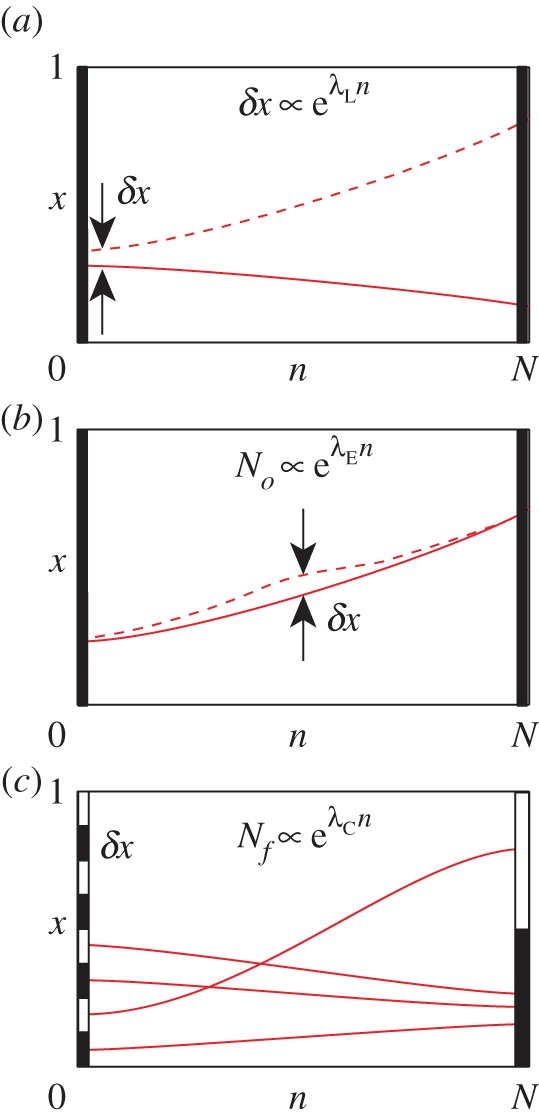
The complexity of a nonlinear map of the unit interval typically increases exponentially with iteration number n. The Lyapunov exponent λ_L quantifies the divergence δx of nearby orbits (a). The topological entropy λ_E = h_T quantifies the number N_o of distinguishable orbits differing by at least δx at some step n (b). The computing exponent λ_C measures the number N_f of distinguishable functions the map can implement given the coarseness δx of the encoding and decoding, which represents different inputs and outputs in different sections of the state space (c). (Online version in colour.)

The rich dynamics of nonlinear systems facilitate the implementation of different computations. For example, if the nonlinear system were chaotic, the future states would be highly sensitive to the initial conditions [25]. A very small change in the initial condition would dramatically change the future states and, therefore, the type of computation that the chaotic system instantiates [5,8,14,26]. This suggests a conceptual connection between the amount of computation a nonlinear system can perform and the Lyapunov exponent of the same system. However, chaos is not a necessary condition for computation. Even in non-chaotic regimes, the nonlinear convolutions of an iterated map, as in figure 3, can scramble orbits among partitions of the invariant set and thereby create diverse functions.

Figure 3.

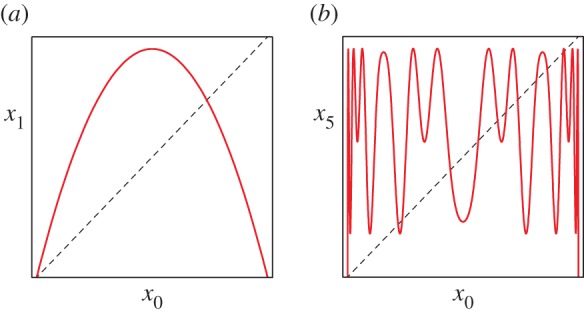
Even a simple nonlinear map (a) gets complicated after only five iterations (b). (Online version in colour.)

(b). Definitions

To motivate the computing exponent definition, consider a dynamics-based computing example [5,8]. If the dynamical system is the nonlinear map of the unit interval

3.2

where p is a bifurcation parameter, then N-fold iterations of the map define binary functions

3.3a

by

3.3b

where the data and the controls , where . One possible encoding is

3.4

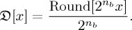
where the data bits are higher and controls bits are lower so function inputs are clustered together. (Alternately, if the data and control bits are interchanged, data bits are lower and control bits are higher so function inputs are spread out.) One possible decoding is

3.5

From a digital logic viewpoint, the map M_p thereby instantiates a family of discrete functions. The n_d data bits comprise inputs. The n_c control bits create up to functions by shuffling those inputs. The n_b base bits define the disjoint unit interval [0,1] outputs: for example, B = 2¹ = 2 creates Boolean functions with two possible outputs, while B = 2⁴ = 16 creates hexadecimal functions with 16 possible outputs.

Abstract this definition, and use symbolic dynamics to define the computing exponent. For granularity, partition an invariant interval into B disjoint subsets, and let be the symbol representing x_n ∈ A. Choose C × D initial conditions and apply the n-fold iterated map to induce the output symbolic vector . Group the components of the output vector into a collection of C sets of D symbols. Let N_f ≤ C be the cardinality of the collection, which typically contains duplicates. In computer simulations, we observe that the number of unique sets N_f increases exponentially with iteration number n (until it plateaus due to the finite number of initial conditions). The computing exponent is the least upper bound over all initial parameters of the logarithm of the function number N_f.

As an example, choose n_d = 2 data bits and n_c = 3 control bits, with data high (yellow highlight) and controls low (cyan highlight), to create C × D = 2²2³ = 2⁵ = 32 binary initial conditions in 2³ = 8 columns

where each column yields the domain of a function. Normalize each initial condition to the unit interval [0,1] by dividing by C × D = 32 to get the decimal initial conditions

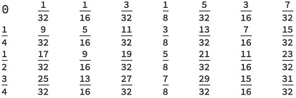
Dynamically evolve each initial condition (by the equation (3.6) tent map with n = 5 iterations at parameter p = 1.7) to get the approximate decimal numbers

Using n_b = 1 base bits, decode each result by rounding to 0 or 1 to get the eight binary outputs

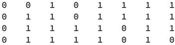
where each column is the range of a function. Convert each column construed as a binary number into a decimal number

Take the union of these numbers to eliminate duplicates and find

The cardinality N_f = 6 of this set is the number of unique functions. One such function f_c[d] is

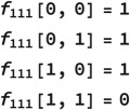
Similarly, use symbolic dynamics to define the topological entropy. As before, given a map M_p, partition an invariant interval into B disjoint subsets, and let σ_n ∈ {0,1,…,B−1} be the symbol representing x_n ∈ A. Choose initial conditions x₀ and apply the map n times to each to induce symbolic orbits. Let N_o ≤ N_i be the cardinality of the set of orbits. We observe that the number of unique orbits N_o increases exponentially with iteration number n (until it plateaus due to the finite number of initial conditions). The topological entropy is the least upper bound over all parameters of the logarithm of the orbit number N_o.

Although the topological entropy and the computing exponent are defined similarly, two apparent differences exist: when counting functions and orbits, the function number depends only on the final symbols while the orbit number depends also on the intermediate symbols; furthermore, the function number depends only on groups of final symbols, not on the final symbols individually. Because the set of functions is a fair sample of the set of orbits, we expect the computing exponent to be similar to the topological entropy, and in fact numerically we observe and we conjecture that the final equality is true in general.

(c). Numerical examples

The approach we use in this paper to estimate the computing exponent is a kind of ‘analysis by synthesis’ in the sense that we analyse and measure the computing power of the system by actually trying different configurations and counting the number of different functions that the system in these different configurations can implement. Of course, we cannot apply and try all possible configurations in a system with continuous variables; however, we can use a subset of these configurations to get a measure on the number of different observed functions, and estimate the rate at which the number of these functions increases as evolution time increases. This rate, which is an exponent, and we named it the computing exponent, is independent of the details of the analysis by synthesis method for its estimation, such as the size of data input n_d, or the size of control inputs n_c or the base of the computation (the number of levels for each symbol). That being said, these parameters should be adjusted carefully so that the numerical method can estimate a relatively precise value for the computing exponent. As an example, imagine we want to estimate the computing exponent of a dynamical system by implementing two-input, one-output digital functions, where the base is 2. There are just 16 different such functions, and when we plot the number of observe functions for different iteration numbers, it will quickly saturate to its maximum possible number after perhaps one or two iterations. As a result we will not be able to observe this exponential increase in the number of functions over the iteration number for a large window to be able to estimate the exponent out of it.

We numerically estimate the computing exponent, topological entropy and Lyapunov exponent for two famous one-dimensional maps, the tent map and the logistics map. Although these two maps are topologically conjugate [27], the former is piecewise linear and has multiple exactly solvable properties, while the latter has a generic quadratic maximum. We obtain similar results with other nonlinear maps.

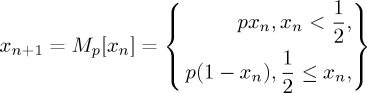
Define the tent map by

3.6

where the state 0 ≤ x_n ≤ 1 and the bifurcation parameter p determines the type of dynamics. In the interval 1 ≤ p ≤ 2, chaos is possible and the tent map topological entropy and Lyapunov exponent can be exactly calculated and are the same, λ_E = λ_L = ln p ≥ 0. Furthermore, the tent map computing exponent can also be exactly calculated. For p = 2, the tent map is a nonlinear transformation of the bit shift map. Hence, the length of the graph, the number of periodic orbits, the number of turning points and the number of state space partitions double with each iteration. Consequently, the number of functions doubles with each iteration, and so . More generally, for the tent map, similar behaviour holds on average, and plausibly so .

Using the definitions of §2, we numerically estimate the number of orbits N_o and the number of functions N_f versus the number of map iterations n. For large parameters, optimal fits to the exponentially increasing regions of number N versus iteration n before the plateau, as in figure 4a plots, estimate the topological entropy and the computing exponent. Hexadecimal base B = 2⁴ = 16 provides the necessary resolution of the tent map's narrow attractor at small bifurcation parameter values p, according to figure 4a, inset. The exponents of figure 4b agree that . These relationships are consistent with Pesin's theorem [28], which equates the entropy of a dynamical system with its total expansion rate. The close agreement between theory and numerics in figure 4b implies that even a single set of evenly spaced initial conditions can produce good estimates of the topological entropy and the computing exponent.

Figure 4.

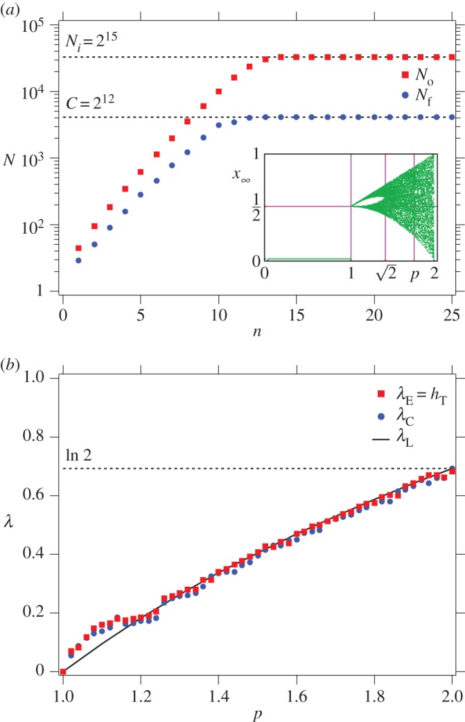
(a) Tent map logarithm of function number N_f and orbit number N_o versus iteration number n for bifurcation parameter p = 1.76. As in encoding equation 3.3(a), functions have n_d = 4 data bits high and n_c = 12 control bits low, orbits have n_i = 15 initial bits, and both use hexadecimal base b = 2⁴ = 16 intervals. Slopes before the plateaus estimate the entropy and computing exponents. Inset is the bifurcation diagram. (b) Chaotic tent map topological entropy λ_E = h_T estimate (red squares), computing exponent λ_C estimate (blue discs) and Lyapunov exponent theory (grey curve) versus bifurcation parameter p. Parameters are the same as in (a). (Online version in colour.)

Define the logistics map by

3.7

where the state 0 ≤ x_n ≤ 1, and the bifurcation parameter p determines the type of dynamics. In the interval , chaos is possible and the logistics map topological entropy and Lyapunov exponent can be positive. (Although the Lyapunov exponent remains negative for a dense set of parameters p.)

Again using the definitions of §2, including the equation 3.3(a) encoding, for a choice of finite parameters, we count the number of orbits N_o and the number of functions N_f versus the number of map iterations n. Optimal fits to the exponentially increasing regions of number N versus iteration n before the plateau, as in figure 5a plots, estimate the topological entropy and the computing exponent. Binary base B = 2 provides adequate resolution, according to figure 5a, inset. The exponents of figure 5b are again consistent with . We do not observe the topological entropy or the computing exponent dipping in periodic windows, such as the famous period-3 window beginning at . This may relate to the many unstable periodic orbits acting as repellers in these parameter regions.

Figure 5.

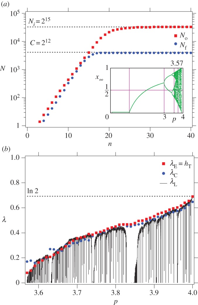
(a) Logistics map logarithm of function number N_f and orbit number N_o versus iteration number n for bifurcation parameter p = 3.8. As in encoding equation 3.3(a), functions have n_d = 4 data bits high and n_c = 12 control bits low, orbits have n_i = 15 initial bits, and both use binary base B = 2 intervals. Slopes before the plateaus estimate the entropy and computing exponents. Inset is the bifurcation diagram. (b) Chaotic logistics map topological entropy λ_E = h_T estimate (red squares), computing exponent λ_C estimate (blue discs) and Lyapunov exponent theory (grey curve) versus bifurcation parameter p. Parameters are the same as in (a). (Online version in colour.)

(d). Applications

The computing exponent measures a kind of complexity that is of both theoretical and practical interest. Nonlinear systems are ubiquitous and so the computing exponent can measure and quantify Nature's complexity in terms of computing power. In addition, the computing exponent can guide engineers to select parameters that optimize dynamics-based computing [7,29].

4. Conclusion

Dynamical systems naturally and intrinsically have computational capability. Since nonlinear dynamical systems have a very rich, complex dynamics, their computational capabilities are also enormous. We discussed how a nonlinear dynamical system can perform computation. And we studied the amount of computation that can be instantiated by such nonlinear dynamical systems. We demonstrated that the number of functions N_f that a nonlinear map M_p can instantiate exponentially increases with time and related the corresponding computing exponent λ_C to the system's topological entropy λ_E = h_T and Lyapunov exponent λ_L. We argued that the computing exponent and the topological entropy are numerically equal, despite their distinct definitions, so that the number of orbits and functions increase at the same rate.

We highlighted an important but subtle connection between a nonlinear system's Lyapunov and computing exponents. The Lyapunov exponent characterizes the average rate of exponential divergence of nearby orbits, whereas the computing exponent characterizes the exponential increase in the number of observed functions, instantiated and programmed by perturbing the system's initial conditions. The convolutions of the nonlinear mapping generate new functions often—but not always—in response to the divergence of nearby orbits. Thus, the computing and Lyapunov exponent are related by conceptually distinct complexity measures that can and do differ for some parameter ranges.

More generally, the science of nonlinear dynamics allows us to transform, control, synchronize, use and exploit complex dynamics. In this way, cybernetical physics enables nonlinear dynamics to be an engine of computation, which can be of great importance in the era in which Moore's law is failing and the search for alternative approaches to increase the performance of computers is at its peak.

Authors' contributions

B.K. contributed the idea of the computing exponent and connected this computational measure to the dynamical system's invariant measure. J.F.L. connected the computing exponent to the topological entropy and improved the numerical methods to estimate it. W.L.D. contributed the foundational idea of dynamics or chaos computing. All three authors contributed to drafting and revising the paper.

Competing interests

We have no competing interests.

Funding

B.K. and W.L.D. gratefully acknowledge support from NCSU under grant no. 201584-70677.

References

- 1.Conrad M. 1986. What is the use of chaos? In Chaos (ed. Holden A.). Manchester, UK: Manchester University Press. [Google Scholar]
- 2.Ditto WL, Pecora LM. 1993. Mastering chaos. Sci. Am. 269, 78–84. ( 10.1038/scientificamerican0893-78)8266061 [DOI] [Google Scholar]
- 3.Andrievskii BR, Fradkov AL. 2003. Control of chaos: methods and applications. I. Methods. Autom. Remote Control 64, 673–713. ( 10.1023/A:1023684619933) [DOI] [Google Scholar]
- 4.Andrievskii BR, Fradkov AL. 2004. Control of chaos: methods and applications. II. Applications. Autom. Remote Control 65, 505–533. ( 10.1023/B:AURC.0000023528.59389.09) [DOI] [Google Scholar]
- 5.Kia B, Lindner JF, Ditto WL. 2015. Nonlinear dynamics based digital logic and circuits. Front. Comput. Neurosci. 9, 269 ( 10.3389/fncom.2015.00049) [DOI] [PMC free article] [PubMed] [Google Scholar]
- 6.Fradkov AL. 2007. Cybernetical physics, pp. 1–16. Berlin, Germany: Springer. [Google Scholar]
- 7.Sinha S, Ditto W. 1998. Dynamics based computation. Phys. Rev. Lett. 81, 2156 ( 10.1103/PhysRevLett.81.2156). [DOI] [Google Scholar]
- 8.Kia B, Lindner JF, Ditto WL. 2016. A simple nonlinear circuit contains an infinite number of functions. IEEE Trans. Circuits Syst. II 63, 944–948 ( 10.1109/TCSII.2016.2538358) [DOI] [Google Scholar]
- 9.Langton CG. 1990. Computation at the edge of chaos: phase transitions and emergent computation. Physica D 42, 12–37. ( 10.1016/0167-2789(90)90064-V) [DOI] [Google Scholar]
- 10.Crutchfield JP. 1994. The calculi of emergence: computation, dynamics and induction. Physica D 75, 11–54. ( 10.1016/0167-2789(94)90273-9) [DOI] [Google Scholar]
- 11.Moore C. 1990. Unpredictability and undecidability in dynamical systems. Phys. Rev. Lett. 64, 2354 ( 10.1103/PhysRevLett.64.2354) [DOI] [PubMed] [Google Scholar]
- 12.Kůrka P. 1995. Simplicity criteria for dynamical systems. In Analysis of dynamical and cognitive systems (ed. SI Andersson), pp. 189–225. Berlin, Germany: Springer. [Google Scholar]
- 13.Delvenne J, Kůrka P, Blondel VD. 2004. Computational universality in symbolic dynamical systems. In Machines, computations, and universality (ed. M Margenstern), pp. 104–115. Berlin, Germany: Springer. [Google Scholar]
- 14.Kia B, Spano ML, Ditto WL. 2011. Chaos computing in terms of periodic orbits. Phys. Rev. E 84, 036207 ( 10.1103/PhysRevE.84.036207) [DOI] [PubMed] [Google Scholar]
- 15.Kia B, Dari A, Ditto WL, Spano ML. 2011. Unstable periodic orbits and noise in chaos computing. Chaos 21, 047520 ( 10.1063/1.3664349) [DOI] [PubMed] [Google Scholar]
- 16.Kia B, Kia S, Lindner JF, Sinha S, Ditto WL. 2014. Noise tolerant spatiotemporal chaos computing. Chaos 24, 043110 ( 10.1063/1.4897168) [DOI] [PubMed] [Google Scholar]
- 17.Schaller RR. 1997. Moore's law: past, present and future. IEEE Spectrum 34, 52–59. ( 10.1109/6.591665) [DOI] [Google Scholar]
- 18.Mitchell WM. 2016. Why the semiconductor industry will soon abandon its pursuit of Moore's law. Now things could get a lot more interesting. Nature 530, 144–147.26863965 [Google Scholar]
- 19.Romero ME, et al. 2014. Universal set of CMOS gates for the synthesis of multiple valued logic digital circuits. IEEE Trans. Circuits Syst. I 61, 736–749. ( 10.1109/TCSI.2013.2284187) [DOI] [Google Scholar]
- 20.Kia B, Mobley K, Ditto WL. 2016. TBA, an integrated circuit design for dynamics-based reconfigurable logic bloc. IEEE Trans. Circuits Syst. II Express Briefs PP, 1 ( 10.1109/TCSII.2016.2611442) [DOI] [Google Scholar]
- 21.Lloyd S. 2001. Measures of complexity: a nonexhaustive list. IEEE Control Syst. Mag. 21, 7–8. ( 10.1109/MCS.2001.939938) [DOI] [Google Scholar]
- 22.Lloyd S. 2002. Computational capacity of the universe. Phys. Rev. Lett. 88, 237901 ( 10.1103/PhysRevLett.88.237901) [DOI] [PubMed] [Google Scholar]
- 23.Rosenstein MT, Collins JJ, De Luca CJ. 1993. A practical method for calculating largest Lyapunov exponents from small data sets. Physica D 65, 117–134. ( 10.1016/0167-2789(93)90009-P) [DOI] [Google Scholar]
- 24.Adler RL, Konheim AG, McAndrew MH. 1965. Topological entropy. Trans. Am. Math. Soc. 114, 309–319 ( 10.1090/S0002-9947-1965-0175106-9) [DOI] [Google Scholar]
- 25.Strogatz S. 2006. Nonlinear dynamics and chaos: with applications to physics, biology, chemistry, and engineering. New York, NY: Perseus Publishing. [Google Scholar]
- 26.Pourshaghaghi HR, Kia B, Ditto W, Jahed-Motlagh MR. 2009. Reconfigurable logic blocks based on a chaotic chua circuit. Chaos Solitons Fractals 41, 233–244. ( 10.1016/j.chaos.2007.11.030) [DOI] [Google Scholar]
- 27.Alligood K, Sauer TD, Yorke JA. 1997. Chaos: an introduction to dynamical systems. Berlin, Germany: Springer. [Google Scholar]
- 28.Pesin YB. 1977. Characteristic Lyapunov exponents and smooth ergodic theory. Russ. Math. Surv. 32, 55–114. ( 10.1070/RM1977v032n04ABEH001639) [DOI] [Google Scholar]
- 29.Prusha BS, Lindner JF. 1999. Nonlinearity and computation: implementing logic as a nonlinear dynamical system. Phys. Lett. A 263, 105–111. ( 10.1016/S0375-9601(99)00665-9) [DOI] [Google Scholar]