Metal Ion Modeling Using Classical Mechanics

Abstract

Metal ions play significant roles in numerous fields including chemistry, geochemistry, biochemistry, and materials science. With computational tools increasingly becoming important in chemical research, methods have emerged to effectively face the challenge of modeling metal ions in the gas, aqueous, and solid phases. Herein, we review both quantum and classical modeling strategies for metal ion-containing systems that have been developed over the past few decades. This Review focuses on classical metal ion modeling based on unpolarized models (including the nonbonded, bonded, cationic dummy atom, and combined models), polarizable models (e.g., the fluctuating charge, Drude oscillator, and the induced dipole models), the angular overlap model, and valence bond-based models. Quantum mechanical studies of metal ion-containing systems at the semiempirical, ab initio, and density functional levels of theory are reviewed as well with a particular focus on how these methods inform classical modeling efforts. Finally, conclusions and future prospects and directions are offered that will further enhance the classical modeling of metal ion-containing systems.

1. Introduction

1.1. Relevance of Computer Modeling of Metal Ion-Containing Systems

1.1.1. Importance of Metal Ions

Metals and metal ions are ubiquitous in nature and account for tremendous chemical diversity. In the periodic table, from element 1 (H) to element 109 (Mt), there are 84 metals, 7 metalloids, and only 18 nonmetals. The sum of the abundances of Al, Fe, Ca, Na, K, Mg, and Ti in the earth’s crust is ∼25%. Metals are well-known substances in our daily lives, composing objects from coins to bridges, but the metal objects we touch are metal crystals or alloys. With low electronegativities, metals are easily ionized and highly reactive, allowing them to participate in many unique reactions or catalytic processes. Metals and their ions are distributed widely and play extremely important roles in chemistry, geochemistry, biochemistry, material sciences, etc. Approximately one-third of the structures in the Protein Databank (PDB) contain metal ions.¹ In biology, Na⁺, K⁺, Mg²⁺, and Ca²⁺ help maintain the osmotic pressure of blood;²⁻⁵ they activate/deactivate some enzymes;⁶⁻¹¹ while redox pairs such as Fe²⁺/Fe³⁺ and Cu⁺/Cu²⁺ are essential to metabolic electron transfer processes,¹²⁻¹⁵ just to name a few of the myriad of biological functions of metal ions. Metals are widely used materials in our daily lives; for example, coins are made of Cu, Ag, Au, Al, Ni, and Fe, etc. Moreover, industrial catalysis is no less reliant on metal chemistry: more than 80% of currently used large-scale chemical processes rely on solid catalysts, typically based on the chemistry of transition metals (TMs).¹⁶

1.1.2. Significant Role of Contemporary Computer Modeling

Contemporary computational chemistry is playing an ever-growing role in chemical research, driven by the improved hardware and lithography, which was facilitated by advances in semiconductor materials containing metals and metalloids. As Moore’s law describes, the computational power of central processing units (CPUs) doubles every 18 months.¹⁷ The dramatic increase in computational power makes previously unattainable computations feasible, allowing for the ever-expanding role of computation in science. For example, in the 1940s and 1950s, with very limited computational power available, it was hard to simulate systems beyond the hydrogen atom,¹⁸ while it is now possible to deal with systems containing hundreds of atoms using ab initio quantum mechanics (QM) methods and systems containing millions of atoms through the use of classical mechanics. The development and application of new hardware modalities also remarkably increased computational power. For example, application of graphic processing units (GPUs) in computational chemistry speeds up calculations by at least an order of magnitude over traditional CPUs.^19,20 Development of the Anton supercomputer makes possible routine millisecond MD simulations of small proteins.²¹

Computational methods offer atomic/molecular and electronic-level insights, which are hard or impossible to obtain experimentally, thereby providing a complementary tool to experiment. Computational approaches can help us to better interpret chemical phenomena and also provide prospective insights and new hypotheses for experimentalists. Novel molecules can be rapidly designed and characterized for desired properties prior to the initiation of expensive synthetic efforts. Computation is playing an increasing role in structure-based drug design and discovery²²⁻²⁷ as well as in the materials design field.²⁸⁻³³ Structure-based drug design computational tools have facilitated in the discovery of novel compounds for diseases including HIV,^22,23,25 cancer,²⁶ and hypertension.²⁷ It has also facilitated in the design of novel materials for applications in solar cells,²⁸ solid catalysts,^29,30 semiconductors, and superconductors.³¹⁻³³

1.2. Challenge of Modeling Metal Ion-Containing Species

1.2.1. High Angular Momenta Atomic Orbitals

Unlike the s and p block elements, TMs have d or f orbitals as their outermost orbitals, which can also participate in chemical bonding. As compared to s and p orbitals, d and f orbitals have more electrons and more complicated shapes (due to their higher angular momenta), which result in more complicated chemical bonding characteristics.

1.2.2. Multiple Oxidation States

Furthermore, there are multiple possible oxidation states for a given TM. For example, Mn has oxidation states ranging from −3 to +7 (with +2, +4, and +7 being the most prevalent), while Fe has oxidation states ranging from −4 to +6 (with +2, +3, and +6 being the most prevalent). Ru and Os have an oxidation state of 8 in RuO₄ and OsO₄.³⁴ In 2014, Wang et al. characterized the [IrO₄]⁺ ion experimentally, in which Ir has a +9 formal charge.³⁵ Recently, Yu and Truhlar predicted that [PtO₄]²⁺ could kinetically exist based on theoretical calculations, in which Pt has a +10 oxidation state.³⁶ Furthermore, the higher oxidation states result in highly charged systems that can have pronounced long-range effects, which need to be accurately accounted for in simulations.

1.2.3. Electronic State Degeneracy

Another significant challenge for modeling TM containing systems is their complicated electronic structures, wherein various spin states can be present with relatively close energies. On one hand, it is generally hard to predict the ground state of a TM ion and to accurately calculate the relative energies between the different states. On the other hand, different spin states may exist at the same time or are essentially degenerate, further complicating the electronic structure. It is impossible to model this static correlation effect based on single-reference methods using a single Slater determinant. Different methods including density functional theory and multireference methods will likely be required to model these systems accurately. Beyond the state degeneracy issue, electronic effects including the Jahn–Teller effect and the trans effect exist, making it even more challenging to accurately model TM-containing molecules at the classical level of theory.

1.2.4. Complicated Chemical Bonding and Multiple Coordination Numbers

On the basis of the above, TM-containing species have more complicated chemical bonding patterns than their organic counterparts, causing much of their ability to have flexible and dynamic coordination environments. Chemical bonds are often characterized on a continuum from covalent to ionic: at one extreme, bonds are based on electrons shared between two atoms, while at the other electrons are exclusively held by one atom or the other, and the association is electrostatic in nature. The main group nonmetal elements usually have consistent bonding patterns due to the nature of their covalent bonds. For example, hydrogen and halogen atoms usually just form one bond with other atoms, while oxygen atoms usually have one double bond or two single bonds with other atoms. Two carbon atoms can form a triple bond at the most, which can be understood as one σ bond and two π bonds between the atom pair. While chemical bonding in organic species has its nuances, many general-purpose chemical models have been designed for organic species and biopolymers that are broadly descriptive of their behavior. However, metal ions present much more challenging modeling problems due to their larger coordination numbers (CNs), relatively labile chemical bonding, and diversity of electronic states.

For the main group metal elements, their chemical bonding has more ionic character, which causes them to have both higher and more flexible CNs than the main group nonmetal elements. For example, Ca²⁺ encompasses CNs ranging from 5 to 10 in aqueous solution.³⁷ Moreover, more complicated bonding patterns can appear between TMs and their coordinating ligands. Whereas main-group compounds tend to have strictly covalent or ionic bonding, transition metals form bonds to their ligands nearer the middle of the bonding “spectrum”. These “coordinate bonds” are typically more flexible and easier to break than a covalent bond, facilitating the use of TMs in catalysts. The coordinate bond shares some characteristics with covalent and electrostatic bonds; depending on the atoms involved, some coordinate bonds are more covalent and some are more ionic. For example, TMs can form both σ and π bonds with coordinate atoms. In contrast, the coordinate bonds in Werner-type compounds are more ionic in nature. Overall, these characteristics give TMs more flexible coordination environments than the nonmetal main group compounds. First, as compared to main group nonmetal elements, higher order bonds can be formed between TMs. For example, Cotton et al. found that there is a quadruple bond between two Re atoms in K₂[Re₂Cl₈]₂·H₂O.³⁸ This bond involves a d_x²–p_z hybrid (as a σ bond), two d_xz–d_yz bonding pairs (as two π bonds), and one d_xy–d_xy bonding pair (as another σ bond) in the quadruple bond. Recent computations of Gagliardi and Roos have shown that U₂ has a quintuple bond (see Figure 1), which has all known covalent bond types (electron-pair bond, one-electron bond, and ferromagnetically coupled electrons) in it.³⁹ Nguyen et al. have crystallized a Cr complex with two Cr⁺ ions (with a 3d⁵ configuration) with a 5-fold bond, with a bond distance of only ∼1.84 Å (see Figure 2).⁴⁰ Second, more diversified bond types existed between TMs and ligands. For instance, “yl-ene-yne” type compounds of W and Cr have been characterized, in which there are single, double, and triple bonds formed between the central metal ion and the surrounding coordinating atoms (see Figure 3).⁴¹⁻⁴³ Moreover, TMs can also have flexible CN values: For example, Cu can have a CN of 5 and 6 in aqueous solution where both configurations have similar energies;⁴⁴ zinc ions play structural and catalytic roles with CNs ranging from 4 to 6 in biological systems.⁴⁵

Figure 1.

Active molecular orbitals forming the chemical bond between two uranium atoms. The orbital label is given below each orbital, together with the number of electrons occupying this orbital or pair of orbitals in the case of degeneracy. Reprinted with permission from ref (39). Copyright 2005 Nature Publishing Group.

Figure 2.

Thermal ellipsoid (30%) drawing of Ar′CrCrAr′ (Ar′ means C₆H₃-2,6(C₆H₃-2,6-Prⁱ₂)₂, where Prⁱ means isopropyl). Hydrogen atoms are not shown. Selected bond distances and angles (deg) are as follows: Cr(1)–Cr(1A), 1.8351(4) Å; Cr(1)–C(1), 2.131(1) Å; Cr(1)–C(7A), 2.2943(9) Å; Cr(1)–C(8A), 2.479(1) Å; Cr(1)–Cr(12A), 2.414(1) Å; C(1)–C(2), 1.421(1) Å; C(1)–C(6), 1.423(2) Å; C(7)–C(8), 1.421(1) Å; C(7)–C(12), 1.424(1) Å; Cr(1A)–Cr(1)–C(1), 108.78(3)°; Cr(1A)–Cr(1)–C(7A), 94.13(3)°; C(1)–Cr(1)–C(7A), 163.00(4)°; Cr(1)–C(1)–C(2), 114.34(7)°; Cr(1)–C(1)–C(6), 131.74(7)°; and C(2)–C(1)–C(6), 113.91(9)°. Reprinted with permission from ref (40). Copyright 2005 The American Association for the Advancement of Science.

Figure 3.

Structures of Schrock and Clark’s “yl-ene-yne” complex of refs (41, 42), Wilkinson’s nitride-imido complex (half of the dimer is shown and the chloride bridges to one lithium of a chemically equivalent manganese center) of ref (46), and the NCr(NPh) (NPrⁱ₂)₂ anion of ref (43). Reprinted with permission from ref (43). Copyright 2016 PCCP Owner Societies.

The higher CN values dramatically increase the number of possible compounds that can be generated around a metal center. Flexible bonding makes it hard to simulate diverse chemical bonds with one modeling strategy. Moreover, the number of electronic states available to some metal ions coupled with more flexible bonds results in many configurations having very similar energies that in turn require highly accurate and expensive computational methods to differentiate the subtle differences. In typical force fields for metal ions, parameters are designed for a specific CN found for the metal ion in an environment. Because an individual metal ion can form many complexes with different CNs, which may or may not be close in energy, and may change from one environment to another, it is hard to simulate these systems accurately. Hence, generating a general force field for metal ions becomes more of a challenge. On the basis of the previous discussion, we hope we have lain bare why it is such a challenge to model metal-containing compounds.

1.3. Impact of the Dearth of Experimental Data

1.3.1. Experimental Challenges

Unfortunately, there are limited experimental data about TM species, which slows the development of accurate theoretical methods to model TM-containing compounds. For example, both the number and the accuracy of experimentally derived heats of formation (HOFs) for TM-containing molecules are modest when compared to what is available for organic compounds. In the work of Jiang et al., they benchmarked the correlation consistent composite approach for transition metals (ccCA-TM) composite method against one of the biggest data sets of experimental HOFs of TM species.⁴⁷ 193 out of 225 entries in the data set were used during the benchmark calculations. As compared to the number of possible TM-containing molecules that could exist, this number represents a rather paltry validation set. Figure 4 showed the mean absolute deviations (MADs) of the ccCA-TM method toward subsets of the experimental data combined with different upper limits of uncertainties. We can see that there are very few (only 32) experimental data points that have accuracies within what is termed “chemical accuracy” (which is ±1.0 kcal/mol). Meanwhile, they found that the MAD of the ccCA-TM method increases along with the upper error limit of the experimental data set they used (see Figure 4), further demonstrating the challenge of using experimental data with higher uncertainties. These results indicate that to impel theoretical methods forward, extensive and highly reliable experimental data will be essential. Because it is challenging to obtain thermodynamic experimental data for TM species to chemical accuracy, the ability for computational methods to advance will be hindered as well.

Figure 4.

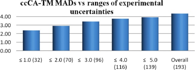
MADs of the ccCA-TM composite method with respect to experimental heats of formation. Unit is kcal/mol along the Y axis. The value in brackets represents the number of data points in the subset. Reprinted with permission from ref (47). Copyright 2011 American Chemical Society.

Another challenging issue is the way in which accurate hydration free energies (HFEs) are obtained for ions. Chemists determine the HFE of a single ion based on experimentally determined HFE values of salts coupled with theoretical assumptions. In particular, the HFE of the proton is usually used as a reference by which the rest of the HFEs are scaled. However, this value has been assigned a range of values covering more than 10 kcal/mol. Meanwhile, there are also other issues that should be considered, including the difference between intrinsic and absolute HFE values, if one wants to accurately model HFE values. Because molecular dynamics (MD) simulations usually employ periodic boundary conditions (PBCs), which do not have an interface, the intrinsic HFE, other than real HFE values, are usually obtained. Related discussions can be found in the work of Grossfield et al.⁴⁸ and in the work of Lamoureux and Roux.⁴⁹ Another issue is that ion parametrization is performed under infinite dilution, while in high concentration solutions, ion pair interactions are important.

1.3.2. Inconsistencies between Experimental and Computational Data

Another aspect that restricts the development of TM modeling is inconsistencies between the available experimental and computational data. For example, X-ray diffraction (XRD) data are always based on the crystal phase.⁵⁰ These crystals are packaged with numerous adjacent unit cells. In QM or molecular mechanics (MM) modeling efforts, the calculation is usually performed in the gas phase without inclusion of crystal packing effects. Moreover, XRD refinement determines the center of the electronic cloud but not the nuclear position, which can be influenced by lone pairs and highly electron-attracting/-donating groups.⁵¹ In contrast, theoretical methods normally use the position of the atomic nuclei. Meanwhile, using experimental data directly may introduce inaccuracies due to different interpretations of the data. For example, the van der Waals (VDW) radii used in X-ray studies are based on the distance of nearby atoms, which are influenced by the crystal packing, while the theoretical chemist treats the VDW radii sum as the energy minimum of two isolated particles.⁵¹ Under these circumstances, assessment of theoretical results based on experimental data may be biased. Moreover, experimental thermochemical data are more often given as free energy values. However, theoretical computation of free energy changes requires extensive sampling, which is still challenging, especially for macromolecular systems.⁵⁰ Therefore, direct comparison between the theoretical and computational data becomes more difficult.

1.4. Scope of This Review

This Review covers the theoretical and computational work on metal ion modeling reported in the past several decades, with a focus on metal ion modeling employing classical force fields. Because quantum calculations are usually used for parametrization and to benchmark metal ion force fields, we briefly review extant QM modeling strategies with respect to metal-containing systems in section 2. Next, we review the widely used nonbonded and bonded approaches to classical modeling of metal ions in sections 3 and 4, respectively. We then summarize the cationic dummy atom and combined models in section 5. These two models are presented separately from the bonded and nonbonded models because they form a distinct set of “semibonded” models. Subsequently, we review several widely used polarizable models in section 6, while in section 7 we review classical models based on the angular overlap model (AOM) and valence bond (VB) theory. Finally, we summarize our conclusions and perspectives on the prospects of this research field in section 8. While we strive to give a balanced review of the field, we realize that due to the limits of our knowledge omissions might occur, for which we make our apologies. Note that the dates listed in the main text represent the year of publication in the original article, which may differ from the year when the article appeared in press. For example, the original paper describing the 12-6-4 LJ-type nonbonded model for divalent metal ions was published online in October of 2013, while it appeared in print in 2014 in the Journal of Chemical Theory and Computation. Hence, we refer to the work as being reported in 2014.

1.5. Previous Reviews

A broad range of reviews regarding the computational modeling of metal ions have been published in the past several decades. Below, we summarize some extant reviews for the sake of the readers who want to trace back through the relevant literature.

1.5.1. Quantum Mechanics Methods

There are a number of reviews concerning TM chemistry that have been published in Chemical Reviews. Holm and Solomon coedited a series of reviews largely focused on experimental studies of bioinorganic enzymes.^{12−15,45,52−71} Davidson edited a series of reviews on QM modeling of TM-containing systems in 2000,⁷²⁻⁸⁵ which summarized the development of ab initio and DFT methods to date. In total, 13 articles on various topics of QM TM modeling were included.⁷³⁻⁸⁵ Holm and Solomon edited another series of reviews on biomimetic inorganic chemistry,⁸⁶⁻¹¹² of which there were couple of reviews on theoretical topics. Noodleman et al. reviewed QM studies of enzyme reaction mechanisms,¹⁰⁴ and Solomon et al. reviewed the electronic structure of models of clusters found in blue copper proteins from both experimental and theoretical points of view.¹⁰⁸ As a sequel to their successful series of reviews in 1996,⁵² Holm and Solomon edited another series of articles on bioinorganic enzymology.^113−123 In the series of reviews about theoretical calculations on large systems edited by Gordon and Slipchenko in 2015,¹²⁴ Blomberg et al. reviewed QM studies of the mechanisms of a series of metalloenzymes.¹¹⁴ Fernando et al. reviewed QM calculations on metal-containing systems including metal, metal oxide, and metal chalcogenide clusters,¹²⁵ which focuses on the structure and physical properties of metal-containing clusters, but did not cover the studies of bulk or surface properties in periodic systems. Finally, Odoh et al. recently reviewed QM studies of metal–organic frameworks (MOFs).¹²⁶

Besides the aforementioned collections of relevant review articles, several other germane reviews have been published in the last several decades. Rode et al. summarized their QM simulation work on ion solvation in 2004.¹²⁷ They used QM MD simulations, which include “quantum effects” and, consequently, provide detailed insights into the ion solvation process. Deeth reviewed the application of DFT methods to the modeling of the active sites and mechanisms of metalloenzyme systems in 2004.¹²⁸ In his review, he discussed factors for designing suitable models and described overall strategies for calculations on these model systems. In 2005, Shaik et al. reviewed the available theoretical work on cytochrome P450 enzymes.¹²⁹ In 2006, Noodleman and Han reviewed DFT methods applied to spin-polarized and spin-coupled systems and DFT applications to different states of redox-active and electron transfer metalloproteins,¹³⁰ while Neese reviewed the application of DFT and time-dependent DFT methods to bioinorganic chemistry.¹³¹ Hallberg reviewed the DMRG method and its applications to various areas including physics and chemistry also in 2006.¹³² In 2009, Cramer and Truhlar reviewed the DFT method and its application to TM chemistry.¹³³ Multiple topics were covered including the effect of DFT functional choice, available software and validation tests, combined with representative applications to different TM-containing systems. Aullón and Alvarez reviewed the relationship of atomic charge and formal charge in TM compounds based on DFT studies on four-coordinated TM complexes.¹³⁴ In 2010, Shaik et al. reviewed QM/MM studies on P450 enzymes.¹³⁵ In 2011, Hofer et al. reviewed studies relating to the hydration of highly charged ions.¹³⁶ In this Review, they concluded that the combination of accurate QM simulation with experimental research would be necessary to obtain highly reliable insights into the solvation of these ions. In 2012, Sameera and Maseras gave an overview of DFT and DFT/MM studies of TM catalysis,¹³⁷ while in 2014, Tsipis reviewed DFT modeling of coordination chemistry.¹³⁸ In the latter, several general suggestions were provided regarding how to choose a DFT functional suitable for the problem at hand.

1.5.2. Unpolarized Force Fields

There are a few reviews on classical modeling of inorganic complexes published several decades ago. For example, Brubaker and Johnson reviewed MM modeling in coordination chemistry in 1984.¹³⁹ Hancock and Martell reviewed MM modeling strategies for application to ligand design for metal ion complexation in 1989.¹⁴⁰ Comba reviewed MM-based studies on metal ion selectivity in 1999.¹⁴¹ Limitations and the reasons for the failure of some of the modeling efforts were discussed along with their possible solutions. Norrby and Brandt reviewed parametrization strategies for deriving MM parameters for coordination complexes in 2001.¹⁴² Topics on model setup, target choice, parameter refinement, and force field validation were covered in the review. Banci reviewed MD simulation work on metalloproteins,¹⁴³ and Comba and Remenyi reviewed MM-based modeling of inorganic compounds both in 2003.¹⁴⁴ For the later, studies on blue copper proteins were used as a case study, while the pros and cons of QM, QM/MM, and MM models were discussed in detail. Jungwirth and Tobias have reviewed classical modeling of ions (for both unpolarized and polarizable force field models) at the air/water interface.¹⁴⁵ Comba, Hambely, and Bodo coauthored a book entitled “Molecular Modeling of Inorganic Compounds” in 2009.¹⁴⁶ Zimmer reviewed classical MM-based simulations of bioinorganic systems and highlighted work on methyl coenzyme-M reductase and urease as example cases.¹⁴⁷ Sousa et al. discussed the difficulties of modeling metalloenzymes using MD simulation and gave an overview of the typical modeling strategies used to solve this problem in 2010.¹⁴⁸ A modeling study of a zinc-containing metalloenzyme-farnesyltransferase using the bonded approach was used to illustrate this modeling strategy. In 2011, Leontyev and Stuchebrukhov reviewed the “molecular dynamics in electronic continuum” method (a charge scaling technique) they developed.¹⁴⁹ In 2012, Dommert et al. reviewed unpolarized, polarizable, and CG force fields for ionic liquids with a focus on the imidazolium-based ionic liquids.¹⁵⁰ In 2012, Riniker et al. reviewed coarse-grained (CG) models for simulating biomolecules, in which they generalized the “coarse-graining” concept and discussed the basic principles involved in developing CG models based on fine-grained models.¹⁵¹ Marrink and Tieleman reviewed the popular MARTINI force field in 2013.¹⁵² In 2015, Nechay et al. reviewed their work on metalloprotein modeling using the QM/discrete molecular dynamics (DMD) approach.¹⁵³ Li et al. reviewed simulation work on metal ion coupled protein folding.¹⁵⁴ Finally, in 2016, Heinz and Ramezani-Dakhel reviewed molecular simulation work on inorganic–bioorganic interfaces.¹⁵⁵ Kmiecik et al. reviewed CG models for proteins and summarized a range of related applications.¹⁵⁶ Cho and Goddard reviewed studies of metalloproteins from the theoretical and experimental points of view in their book.¹⁵⁷

1.5.3. Polarizable Force Fields

Because there are very few extant review articles specific to the modeling of metal ions using polarizable force fields, we decided to highlight a number of reviews on polarizable force fields that have appeared regardless of their overall relevance to metal ion-containing systems. In this way, interested readers can gain entry into this rapidly developing field.

In the collection of Chemical Reviews articles edited by Holm and Solomon in 1996,⁵² one article by Stephens et al. focused on theoretical calculations of the redox potentials of Fe–S proteins using the protein dipole Langevin dipoles model.¹³ Halgren and Damm summarized work on polarizable force fields up to ∼2001.¹⁵⁸ In 2002, Rick and Stuart reviewed the strategies of incorporating polarizability into classical modeling while focusing on the use of polarizable force fields in MD and Monte Carlo (MC) simulations.¹⁵⁹ Ponder and Case reviewed the available protein force fields (both unpolarized and polarizable) in 2003.¹⁶⁰ Mackerell gives a short review on polarizable force fields as part of his review of empirical force fields in 2004.¹⁶¹ Friesner has also reviewed the development of polarizable force fields in 2005.¹⁶² Patel and Brooks summarized their work on the development and application of the CHARMM fluctuating charge (FQ) model in 2006.¹⁶³ Gresh et al. gave an overview of the formulation and applications of the sum of interactions between fragments computed ab initio (SIBFA) method in 2007.¹⁶⁴ Warshel et al. critiqued the development of macroscopic polarizable force fields and emphasized the importance of polarization effects in application studies in their review in 2007.¹⁶⁵ Cieplak et al. sketched out the development and application of polarizable force fields for macromolecular simulations in 2009.¹⁶⁶ They reviewed unpolarized force fields, followed by intermolecular interactions studied by QM methods, and then polarizable force fields. Loopes et al. summarized the theories, extended Lagrangian integrators, and application studies of polarizable force fields in 2009.¹⁶⁷ Russo and van Duin described the reactive force field (ReaxFF) method and showed an application to a zinc–oxide nanowire in 2011.¹⁶⁸ Gong outlined modeling work of ion-containing systems using the atom-bond electronegativity equalization method (ABEEM) FQ model in 2012.¹⁶⁹ Lamoureux and Orabi, in 2012, reviewed the cation−π interaction modeling with an emphasis on applications to proteins and the Drude oscillator (DO) model they developed.¹⁷⁰ Shin et al. surveyed the use of ReaxFF for simulating complex bonding and chemistry in 2012, with an emphasis on the application of ReaxFF and the charge optimized many-body models.¹⁷¹ An overview of the development and application of reactive potentials was given by Liang et al. in 2013, with an emphasis on the comparison of ReaxFF and the charge-optimized-many-body (COMB) force fields with variable-charge schemes.¹⁷² In 2015, Shi et al. gave a conspectus on the recent progress of different polarizable force fields,¹⁷³ and in the same year Vanommeslaeghe and Mackerell examined recent developments of the CHARMM unpolarized force field and discussed the CHARMM DO force field, with an emphasis on its parametrization scheme.¹⁷⁴ Recently, Lemkul et al. have reviewed the DO model with emphasis on the application of the Drude-2013 model to biological molecules.¹⁷⁵ Senftle et al. reviewed the ReaxFF model, in which its development, applications, and future directions were discussed.¹⁷⁶

1.5.4. Other Models

Landis and co-workers reviewed their SHAPES method in 1995,¹⁷⁷ and Deeth and co-workers have written several reviews and book chapters regarding their ligand field MM (LFMM) method.^178−182

2. Modeling Transition Metal-Containing Species Using Quantum Mechanics

2.1. Challenges

This Review concentrates on force field modeling for metal ions; however, due to the broad adoption of QM methods to derive force field parameters and in QM/MM simulations, we provide a brief review on metal ion modeling using QM methods. A number of more extensive reviews on QM modeling of TM-containing systems are available in the literature for the interested reader.^183−185

QM and QM/MM methods offer detailed insights into intermediates and transition states in catalysis, where these states are hard to understand using experimental tools.¹³⁷ However, it is still challenging to accurately model TM-containing systems using QM calculations. In particular, modeling the multireference characteristic of many TM species using single reference methods is not handled correctly because they do not address static correlation.

Besides modeling molecules, it is hard to simulate the metal atoms from the middle TM series. Here, we treat the Ni atom as an example. The atomic excitation energies of Ni for 3d⁹4s¹–3d⁸s² (³D–³F) and 3d⁹4s¹–3d¹⁰ (³D–¹S) excitations calculated by several different QM approaches are shown in Table 1, together with experimental values. Table 1 shows that the HF method gives significant errors predicting these properties, while multireference methods need to be employed to obtain accurate results.

Table 1. ³D–³F and ³D–¹S Excitation Energies of Ni Based on Several Different QM Methods and from Experiment^a.

	HF188	HF+rel188	SDCI+rel188	SDCI+rel with Davidson correction188	MRCI+rel188	MRCI+rel with Davidson correction188	exp.189
3D–3F	–1.277	–1.637	–0.340	–0.325	–0.086	–0.195	0.03
3D–1S	4.199	4.404	2.484	2.261	1.879	1.843	1.74

^aUnits in eV. Herein, +rel means with relativistic correction, the HF and HF+rel calculations used an uncontracted (20s15p10d6f) basis set, while the rest of the calculations used a (7s6p4d3f2g) basis set; the experimental results were obtained after averaging over the J-components.

Martin and Hay have studied the excitation energies of low-lying states and ionization potentials (IPs) of TMs.¹⁸⁶ Relativistic effects were taken into consideration based on the scheme of Cowan and Griffin.¹⁸⁷ They found that the relativistic effect stabilized the “s-electron-rich” configurations, while correlation effects favored the “d-electron-rich” configurations. In their work, it was shown that the numerical HF method without relativistic correction predicted excitation energies for the ³D–³F and ³D–¹S transitions of −1.27 and 4.20 eV, respectively, while the relativistic HF method predicted the two values as −1.63 and 4.41 eV, respectively. Bauschlicher et al. systematically investigated different methods for predicting these excitation energies.¹⁸⁸ They found a single reference SDCI approach offered improvement, but the differences when compared to experiment were still considerable (see Table 1). Finally, they showed that the multireference configuration interaction (MRCI) method coupled with large atomic natural orbital (ANO) basis sets could further reduce the errors (see Table 1).

Because the DFT method considers the electron density–energy relationship directly, it incorporates static correlation effectively when modeling TM containing systems.¹³³ However, there are a large number of functionals available, and the computational accuracy varies widely among them and is property dependent. Hence, the answer to the question of which functional should be used really depends on the system and property one wants to investigate. In general, correlation functionals, which do not attain the homogeneous gas electron limit, are not suggested for pure metal systems,^190,191 while for mixed systems, such as organometallics, this is not a significant limitation.⁸⁴

2.2. Ab Initio Methods

The Hartree–Fock (HF) method is a self-consistent field (SCF) method that was first proposed by Hartree^192,193 and later developed by Fock,¹⁹⁴ Slater,^195,196 etc., resulting in the HF method widely used nowadays. It uses several approximations to solve the Schrödinger equation efficiently for complex systems, including the Born–Oppenheimer, nonrelativistic, linear combination of atomic orbitals (LCAO), Slater determinant, and mean field approximations. However, because it neglects the correlation energy and is a single reference method, it is generally not used for modeling TM-containing systems. Even with these issues, HF methods can be used for force constant derivation with some success.¹⁹⁷ The MP2, CCSD, and CCSD(T) methods include some portion of the correlation energy and are contemporary post-HF work horses. Among them, CCSD(T) with complete basis set (CBS) extrapolation is treated as the “gold standard” for predicting the properties of small organic molecules.¹⁹⁸ It can achieve chemical accuracy (±1 kcal/mol) for atomization energies and reaction enthalpies for small molecules.¹⁹⁹ However, due to its single reference character, CCSD(T) does not afford an accurate representation of “static correlation”. Multiple reference wave function-based methods offer better descriptions but with greatly increased computational cost.²⁰⁰

TM-containing systems are more likely to have strong multireference properties due to the near degeneracy of d orbitals. A well-known multireference TM system is Cr₂, its multireference character making it challenging to simulate using methods employing a single Slater determinant.²⁰¹ However, we note that multireference is not only a characteristic that is relevant to TMs. For example, the C₂ molecule, which has several low-lying excited electronic states, also has strong multireference character. Abrams and Sherrill have explored the limitations of single-reference methods in modeling the multireference C₂ system.²⁰²

Jiang et al. studied the multireference character of 3d TM-containing systems and have discussed the criteria for determining this characteristic.²⁰³ Subsequently, Wang et al. performed related studies for 4d TM-containing species and listed criteria for determining the multireference characteristics of these systems.²⁰⁴

Weaver et al. have investigated the accuracy of the CCSD and CCSD(T) methods for calculating the HOFs of zinc-containing systems.²⁰⁵ The basis sets 6-31G** and TZVP, along with two hybrid basis sets LANL2DZ-6-31G** (same as LACVP**) and LANL2DZ-TZVP, were employed. The 6-31G** basis set showed the best performance in general. The CCSD(T)/6-31G** level of theory showed the best performance for predicting the HOFs of nonalkyl zinc species, while none of the investigated theory combinations could reproduce the HOFs of alkyl zinc compounds accurately. Moreover, it was shown that the CCSD/6-31G** level of theory could best reproduce experimental geometries. However, the coupled cluster (CC) methods did not systematically outperform DFT functionals. For the ZnH and ZnF₂ systems, there are many DFT functionals that gave better predictions with the 6-31G** basis set. In a related work by Weaver and Merz, they investigated the CC method for calculating the HOFs of copper-containing systems.²⁰⁶ The results indicated that there is no correlation between calculating the HOFs accurately and predicting bond lengths precisely. The CCSD(T)/6-31G** level of theory incorrectly predicts the ground state of the CuO compound as a quartet, with an elongated bond length (∼0.29 Å longer than experiment), and afforded an overestimate of the HOF value (∼29 kcal/mol higher when compared to experiment).

In the recent work of Xu et al., they calculated the bond energies of 20 diatomic molecules containing 3d TM elements using four CC-based methods (CCSD, CCSD(T), CCSDT, CCSDT(2)_Q) and 42 DFT functionals, and compared them to the most reliable experimental data.²⁰⁷ They found that the CC methods only offered similar accuracy with, but not necessarily better than, the DFT methods, suggesting that CC methods do not form a benchmark theory for DFT methods. They also found that both CC and DFT methods perform better for single reference systems than for multiple reference systems. Moreover, it was found that CCSD(T) calculations usually underestimate the bond energies, while DFT broken-symmetry calculations usually overestimate these values. Overall, using CCSD(T) results as benchmark values for DFT and other methods should be treated with caution for TM methods.²⁰⁷

Given the limited accuracy of direct prediction based on post-HF methods, the scaled approach is an alternative and offers improved results. For example, Hyla-Kryspin and Grimme have investigated the dissociation enthalpy changes of a number of TM complexes using the MP2, MP3, spin component scaled-MP2 (SCS-MP2), SCS-MP3 methods, and the BP86 density functional, and compared them to experimental data.²⁰⁸ The mean average error (MAE) values of the MP2, MP3, SCS-MP2, SCS-MP3, and BP86 methods are 21.0, 22.3, 11.6, 4.1, and 3.4 kcal/mol, respectively. This indicates the SCS method can correct the erratic behavior of MP2 and MP3 methods, and that DFT showed improved performance in the modeling of these systems.²⁰⁸

Carlson et al. have studied a di-iron complex Fe–Fe–Cl and some analogues with weaker metal–metal bonds (Co–Co, Co–Mn, Co–Fe, and Fe–Mn) using multireference wave function-based methods and DFT functionals.²⁰⁹ They found that a larger active space is necessary to correctly describe the Fe−Fe−Cl system. Full consideration of the 4d orbitals in the active space is needed to correctly describe the electronic delocalization and bonding between the two irons in the Fe–Fe–Cl complex, while truncation of the 4d orbital set causes the inaccurate modeling of some 3d orbitals, and incorrectly predicts the ground spin state. However, for the Co–Co–Cl system, which has more localized metal centers, a full or truncated inclusion of 4d orbitals in the active space affords the same result. They also found that some DFT functionals predict the correct ground spin state, chemical bond, and structural properties of the complexes investigated, while hybrid functionals strongly localized the 3d orbitals and failed to predict the correct spin state ordering, especially for the di-iron complex.

2.3. Composite Methods

The so-called QM composite methods attempt to mimic the accuracy of more expensive high-level QM calculations by using a combination of several procedures with lower computational expense and accuracy.²¹⁰ Pople, Curtiss, and co-workers have developed the Gaussian-1 (G1), Gaussian-2 (G2), and Gaussian-3 (G3) approaches and pioneered this field.^211−214 These approaches were intended to create a “black box” to accurately predict energetic properties including HOFs, IPs, electron affinities (EAs), and proton affinities within ±2 kcal/mol of experimental data.²¹⁰

Subsequent to these methods, Curtiss et al. developed the Gaussian-4 (G4) method.²¹⁵ Mayhall et al. have calculated the enthalpies of formation of 20 3d TM-containing molecules using several composite approaches and DFT functionals.²¹⁶ It was shown that the four composite approaches G4(MP2, rel), G4(rel), G3(CCSD, rel), and G3(CCSD, MP2, rel) have MADs of 2.84, 4.75, 5.81, and 4.85, respectively (here, “rel” represents including corrections for scalar relativistic effects). They proposed that the failure of the G4(rel) method is due to the poor convergence of the MP4 calculations. The B3LYP, PBE, and PW91 functionals showed remarkably different performance: the B3LYP functional yielded a MAD of 4.64 kcal/mol, while the later two functionals showed MADs of more than 20 kcal/mol.

Wilson and co-workers are active in composite approach development for TM systems, and herein we briefly introduce their work. Wilson and co-workers developed the correlation consistent composite approach (ccCA) in 2006.²¹⁰ It is a MP2-based composite method without any parameters. It was shown that the method could accurately predict the energetic properties of main group species (with MAD < 1 kcal/mol)²¹⁷ and s-block systems (with a bigger deviation but still good accuracy).^218,219 In 2007, they used the ccCA approach to study the HOFs of 17 3d TM species.²²⁰ They noted that the amount and accuracy of experimental thermochemistry data were limited, and it is challenging to achieve “chemical accuracy” for both experimental and theoretical thermochemistry.²²⁰ Hence, in light of this, an average deviation of ±3 kal/mol could be considered as “chemical accuracy” for TM thermochemistry. The ccCA method showed a MAD of 3.4 kcal/mol for a training set of 8 TM-containing molecules, similar to the DK-CCSD(T) approach (a CCSD(T)-based composite approach), which yielded a MAD of 3.1 kcal/mol for the same set. However, the agreement between the theoretical values and experimental data is more system dependent, when compared to that of the main group molecules.

DeYonker et al. have used the ccCA method to calculate the HOFs of 147 main group molecules and 52 3d TM complexes in 2009.²²¹ They obtained a MAD for the former set of 0.89 kcal/mol, while the MAD and mean square deviation (MSD) for the later set was 2.85 and 3.77 kcal/mol, respectively.²²¹ It was shown that the DFT results are more system dependent with some of them giving erratic predictions for some cases, while the ccCA method was less system dependent and more consistent. They also pointed out that some of the experimental data need to be revisited based on the ccCA calculations.

Subsequently, Jiang et al. calculated the enthalpies of formation of 225 3d TM species using the ccCA-TM approach and compared them to experimental results.⁴⁷ It was shown that the deviation from experiment decreases only when consideration is made for the uncertainty in the experimental data. The MADs for subsets of TM-containing systems, which have uncertainty upper limits of ±5, ±4, ±3, ±2, and ±1 kcal/mol, were 3.91, 3.74, 3.42, 2.90, and 2.37 kcal/mol, respectively (see Figure 4). Hence, they proposed that the large error from theory is due to less reliable experimental data for TM-containing species relative to organic species.⁴⁷ They also carried out calculations using the B3LYP and M06 functionals for comparison; the MAD of B3LYP for the subsets with different upper limits in uncertainty (±1 to ±5 kcal/mol) are in the range of 12.9–14.1 kcal/mol, while for the M06 method the corresponding values are in the range of 10.5–11 kcal/mol. These results showed that the accuracy of the ccCA-TM composite method outperforms DFT methods.

Laury et al. have carried out calculations of thermochemical properties of 25 molecules containing 4p elements (Ga–Kr) and 30 molecules containing 4d TMs, using the relativistic pseudopotential ccCA (rp-ccCA) method.²²² The rp-ccCA approach needs less time than the ccCA method because a pseudopotential was also employed. The average uncertainty of the experimental HOFs for the 4d TMs is 3.43 kcal/mol. The values obtained from the rp-ccCA method had MADs of 0.89 and 2.89 kcal/mol for molecules containing 4p elements and 4d TMs, respectively. Overall, these results show the ability of the ccCA approach.

2.4. Semiempirical Methods

TMs have significantly more electrons than the first- and second-row elements in the periodic table, resulting in a significant increase in computational cost. While it is challenging to perform ab initio calculations of TM containing systems, semiempirical (SE) methods are efficient and attractive alternatives. SE methods use a minimal basis set to save computational time. Generally the time complexity of SE methods is O(N²) or O(N³), where N is the number of basis set functions.²²³ Hence, SE methods are ∼1000 times faster than the DFT method,²²³ allowing for the treatment of larger systems using modern computational resources.

2.4.1. Neglect of Differential Overlap-Based Methods

Pople and co-workers pioneered the development of SE methods and proposed the complete neglect of differential overlap (CNDO),^224,225 intermediate neglect of differential overlap (INDO),²²⁶ and neglect of diatomic differential overlap (NDDO) methods in the 1960s.²²⁷ These methods use strategies, as their names indicate, to neglect all or some of the differential overlap calculations in the HF method to save on computational time.

Zerner and co-workers pioneered SE method development for TMs: they parametrized the INDO scheme (so-called ZINDO method) not only for the main group elements, but also for the 3d and 4d TMs, and even lanthanides and actinides, from the 1970s to the 1990s.^228−236 It uses a linear combination of two Slater functions to represent the atomic orbitals of the main group elements (K to I) and TMs. It sets the one-center Coulomb integrals on one atom as identical and evaluates them as the difference between the IP and EA of the atom (also known as absolute hardness). Exchange integrals are represented using Slater–Condon parameters. Reference spectra were used to fit some parameters in the scheme. These parameters concentrated more on reproducing spectroscopic and electron-transfer properties.²³⁷ Filatov et al. have proposed and parametrized the CNDO-S² procedure for molecules containing H, C, N, O, and Ni atoms in 1987.²³⁸ Nieke and Reinhold parametrized the NDDO method for 3d TMs in 1984.²³⁹ Subsequently, Filatov et al. developed the NDDO/MC (NDDO for metal compounds) method and parametrized it for H, C, N, O, Co, and Ni atoms in 1992.²⁴⁰

Jug and co-workers developed the SINDO1 method, which is consistent with the symmetrically orthogonalized INDO (SINDO) method that considers the orthogonality of atomic orbital basis sets in calculating related core-Hamiltonian elements.^241−243 The frozen-core strategy was used, and only the electrons of the valence-shell are represented explicitly in the SINDO1 method.^241−243 Jug and co-workers extended and parametrized the SINDO1 method to 3d TM elements in 1992.²⁴⁴ 90 bond lengths, 14 angle values, HOFs of 78 molecules, and IPs of 32 molecules from experiment were used as the reference set for parametrization. The obtained results showed that the SINDO1 method could predict the geometry with considerable accuracy and reproduce the HOFs and IPs semiquantitatively. Later, they developed the modified SINDO (MSINDO) method^245−247 and also parametrized it for 3d TMs. HOFs, IPs, geometries, and dipole moments of more than 200 molecules were treated as the reference set for parametrization.²⁴⁸ Comparison with the SINDO1 method was carried out, and in general the MSINDO method showed substantial improvement over its predecessor. The transferability of these parameters was shown in calculating the binding energies of monohydrates of singly charged 3d TM ions from Ti⁺ to Cu⁺.

2.4.2. Modified Neglect of Diatomic Overlap-Based Methods

Dewar and co-workers played a significant role in the development of SE methods. They developed the modified intermediate neglect differential overlap (MINDO),²⁴⁹ MINDO/2,²⁵⁰ and MINDO/3²⁵¹ methods based on the INDO approximation in 1969, 1970, and 1975, respectively. To improve the overall accuracy of their methods, Dewar and Thiel developed the modified neglect of diatomic overlap (MNDO) method based on the NDDO approximation in 1977.²⁵² Dewar and co-workers parametrized the MNDO method for Sn and Hg in 1984 and 1985, respectively.^253,254 Dewar and Merz parametrized MNDO for Zn in 1986.²⁵⁵ Thiel and Voityuk extended the MNDO scheme to d orbitals (so-called MNDO/d method) and demonstrated improved results.^256,257 In 1996, they parametrized the MNDO/d approach for the second-row elements (except Ar) and group IIB elements (Zn, Cd, and Hg).²⁵⁸ Extensive tests were carried out, and it was again shown that the MNDO/d method outperformed other MNDO-type methods lacking d-orbitals.²⁵⁸

2.4.2.1. AM1 Model

Dewar and co-workers developed the Austin Model 1 (AM1) method in 1985 to better model hydrogen-bonded systems.²⁵⁹ Dewar and Merz extended this method for Zn in 1988, which showed better performance than the MNDO method for this same metal.²⁶⁰ Voityuk and Rösch added d-orbitals to the AM1 method (so-called AM1/d method), parametrized it for Mo, and demonstrated this method’s ability to predict the geometries and HOFs of a series of Mo complexes.²⁶¹ Imhof et al. parametrized the AM1/d method for Mg in metalloenzymes and demonstrated considerable improvement over the AM1 and MNDO/d methods.²⁶² Finally, Clark and co-workers developed the AM1* model for a series of elements including the 3d TMs (except Sc) as well as Al, Zr, Pd, Ag, and Au.^263−269

2.4.2.2. PMx Models

Stewart described the parametric method 3 (PM3) method in 1989^270,271 and extended it to 28 elements including metals such as Be, Mg, Zn, etc., in 1991.²⁷² Ignatov et al. extended the PM3 method to a s,p,d basis set and carried out test calculations on organometallic complexes of Cr in 1996.²⁷³ Børve et al. applied the PM3(tm) method to several catalysts containing Ti, Zr, or Cr in 1997.²⁷⁴ Cundari and Deng parametrized the PM3 method for TMs against experimental structures in 1999.²⁷⁵ Their model showed the ability to predict the geometries of TM complexes, especially for TMs in the left-hand side of the periodic table.²⁷⁵ Stewart have extended the PM3 method creating PM6 in 2007 that covered 70 elements and showed excellent overall performance in predicting HOFs.²⁷⁶ PM7 appeared in 2013, and it showed improved performance over PM6.²⁷⁷ Seitz and Alzakhem used the AM1/SPARKLE, PM3/SPARKLE, and PM6/SPARKLE methods to study more than 650 Ln complexes, which have water coordinating the metal ion in 2010.²⁷⁸

2.4.3. Embedded Atom, Finnis–Sinclair, Sutton–Chen, and Tight-Binding Models

There are three different packing patterns for metals: the body-centered cubic (BCC), face-centered cubic (FCC), and hexagonal close-packed (HCP) structures. Metals in these three packing structures have CNs of 8, 12, and 12, respectively. The packing factors of these three packing modes are 0.68, 0.74, and 0.74, respectively. Different metals may have different packing structures. For instance, metals such as Li, Na, K, V, Cr, Ba, etc., have BCC structures, metals including Al, Cu, Ag, Au, Ni, Pt, Pb, etc., have FCC structures, and Be, Mg, Zn, Cd, etc., have HCP structures.

A number of SE models have been developed for metals and their alloys, including the embedded atom model (EAM),²⁷⁹ Finnis–Sinclair (FS) model,²⁸⁰ Sutton–Chen (SC) model,²⁸¹ and tight-binding (TB) model.²⁸² These models are many-body potentials and are related to the electronic density. Generally, it is more challenging to model BCC metals than FCC and HCP examples. It is also not an easy task to calculate the relative stabilities of the former over the latter two. Below we briefly review several representative approaches.

2.4.3.1. Embedded Atom Model

Daw and Baskes developed the EAM method based on DFT in 1983.²⁷⁹ They have applied it to the hydrogen doped Ni system, and their results showed that fracture stress in metallic Ni could be reduced by hydrogen. Subsequently, they described the formalism of the EAM method.²⁸³ The total potential is shown in eq 1. ρ_h,i is the host density, which is approximated by a sum of atomic densities (see eq 2). ϕ_ij is a short-range pairwise repulsive potential (see eq 3). This potential is represented by the electrostatic interaction of the effective charges of two interacting atoms. Different properties (such as the lattice, elastic constant, etc.) can be derived from the total energy. They parametrized the potential for Ni and Pd metals and applied it to study related impurity, surface, and defect properties.

1

2

3

Foiles et al. have further developed the EAM model for several FCC metals (Cu, Ag, Au, Ni, Pd, and Pt) and their alloys.²⁸⁴ The potentials were fitted to several experimental properties. It was shown that the model reproduces various properties including several issues related to impurities and surface properties.

2.4.3.2. Finnis–Sinclair Model

Finnis and Sinclair developed an empirical N-body model (the FS model) for TMs in 1984.²⁸⁰ The components of the potential function are shown below:

4

5

6

7

Here, the repulsion term is an additive two-body term, representing core–core interactions, while the attractive term is an N-body term that represents the band energy. It mimics TB results by choosing f(ρ_i) as , where ρ_i is the site electronic charge density via summation over the neighboring atoms j into a potential ϕ, and where ϕ(r_ij) can be considered as the sum of squares of hopping integrals.²⁸⁰ Both terms in eq 4 were short-ranged with specified distance cutoffs. The parameters are fitted to lattice constants, cohesive energies, and elastic moduli for 7 BCC TMs. In the original parametrization, they used a parabolic equation for ϕ(r_ij) (a different formulation was used for Cr and Fe) and a quartic polynomial equation for U_rep. It was shown that the model could reproduce different experimental properties and also results based on the TB theory, while offering improvement over the simple pairwise potential.

2.4.3.3. Sutton–Chen Model

Sutton and Chen developed the SC potential on the basis of the Finnis–Sinclair potential in 1990.²⁸¹ They discussed that the description of the VDW potential is as important as modeling the short-range interactions. The function has the form:

8

9

The attractive term is represented by an N-body potential; it can be extended to a pairwise potential when an additional atom approaches the surface at long-range, even as the magnitude of the pairwise potential is influenced by other neighboring atoms. By assigning m = 6, one has a r^–6 representation for the attraction energy at long-range. However, it was shown that the potential always favors the FCC and HCP structures over the BCC one. It was also shown that the SC model could be extended to a pairwise LJ m–n model under a reference density (see eq 10).

10

The only parameters that need to be determined in the equation are ε, σ, m, and n. Sutton and Chen have derived analytical expressions for different experimental properties on the basis of the potential. On the basis of this, they parametrized the potential for 10 FCC metals to reproduce different experimental properties. For these metals, m was determined to be in the range of 7–14, while n was determined to be in the range of 6–8. They also discussed that there are different physical origins for the short-range N-body unsaturated covalent bond and the VDW interaction, even if they are merged into one term in the equation for mathematical convenience.

2.4.3.4. Tight-Binding Model

Cleri and Rosato developed the TB model with second moment approximation (TB-SMA) for FCC and HCP TMs.²⁸² Meanwhile, examples of potential derivations for a few TM alloys were also presented in their work. The potential consists of a band energy term and a repulsive term (see eqs 11–13). The band energy term is a many-body term, while the repulsion term is a pairwise term based on the Born–Mayer equation. In the band energy term (eq 12), ξ represents the effective overlap/hopping integral, which is similar to the format of the FS model that uses the formulation to mimic the results of the TB model. Only A, ξ, p, q, and r₀ are the parameters that need to be determined in the model. They were fitted to reproduce different experimental properties. The model effectively simulates the thermal behavior of TMs. It was shown that through the use of a large cutoff, the model could represent experimental data even at temperatures close to the melting point of the metal, which is usually beyond the capability of a short-range model. However, the potential did not successfully model BCC metals. Other limitations were discussed in the concluding remarks in their work.²⁸²

11

12

13

2.4.4. Self-Consistent Charge Density Functional Tight-Binding Model

Elstner, Cui, and co-workers have performed extensive work developing the self-consistent charge DFTB (SCC-DFTB) method. Siefert et al. proposed the density functional tight-binding (DFTB) method in 1986.²⁸⁵ Elstner et al. followed with the SCC-DFTB method and applied it to organic, biomolecular, and material systems containing light main group elements in 1998.²⁸⁶ The SCC-DFTB method is based on a second-order expansion of the charge density (see eqs 14–17). It uses Mulliken partial charges to represent the charge densities. “Band-structure” energy and a short-range repulsive term, along with a Columbic interaction between the charge fluctuations, were included in this approach. Akin to HF-based SE methods, SCC-DFTB uses a minimal basis set, which limits its accuracy to some extent. One important difference between the SCC-DFTB and SE methods is the former has O(N²) parameters (here N is the element numbers), while the latter only uses O(N).

14

15

16

17

18

Elstner et al. extended the SCC-DFTB method to Zn in 2003,²⁸⁷ where they used a new functional form for the E^rep term (see eq 18). They parametrized it on the basis of B3LYP calculations and tested the parametrization on a series of biologically relevant zinc complexes via calculations on the geometries, relative binding energies, ligand deprotonation energies, and reaction barriers. The results considerably outperformed the PM3 method in many aspects, and good agreement with B3LYP/6-311+G** or MP2/6-311+G** calculations was obtained.

In an examination of the SCC-DFTB and NDDO-based methods, Sattelmeyer et al. showed that the former approach outperformed the latter in some areas when modeling molecules containing C, H, N, and O.²⁸⁸ They observed that the SCC-DFTB method gives better conformational and intermolecular interaction energies but gives less accurate HOFs of ions and radicals. However, none of these methods accurately modeled hydrogen bonds with strengths less than 7 kcal/mol. Moreover, SCC-DFTB was shown to have considerable errors when dealing with S–O and N–O bonds.²⁸⁸

In 2007, Zheng et al. parametrized the spin-polarized SCC-DFTB method for Sc, Ti, Fe, Co, and Ni atoms.²⁸⁹ They carried out the parametrization based on the B3LYP functional with mixed basis sets (SDD plus 6-31G*) and tested the parameters on a series of TM species. The computed results indicated that the parameters accurately modeled structural properties but only qualitatively reproduced energetic properties (such as bond energies and relative energies between different spin states) when compared to the reference B3LYP/SDD+6-31G* level of theory. A parametrization of the Cu ion was reported in 2012 by Bruschi et al. using the spin-polarized SCC-DFTB method.²⁹⁰ The results indicated that the SCC-DFTB method was able to reproduce the energetic sequence of the three most stable Cu(HGGG) (Py) (see Figure 5) isomers in comparison to the BP86/TZVP level of theory.

19

20

Figure 5.

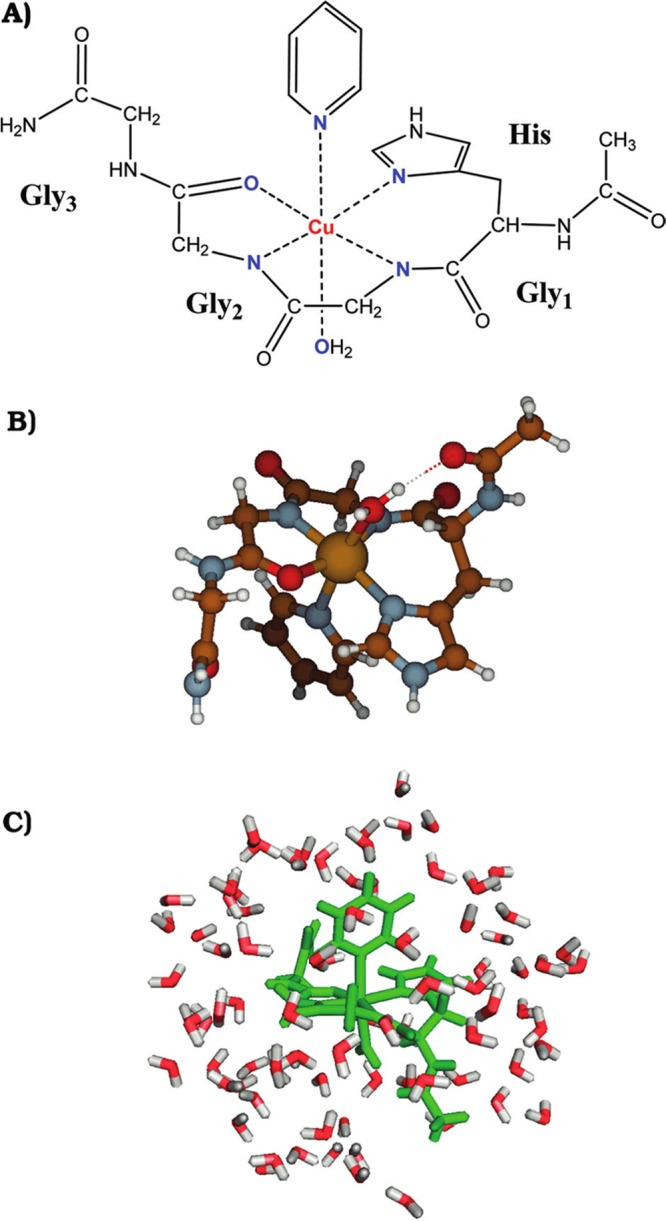
Complex [Cu(AcHG₁G₂G₃NH₂)(Py)(W)] used as a precursor of all of the five- and four-coordinated forms considered in the study of Bruschi et al.²⁹⁰ (A) Schematic representation of the complex; (B) molecular geometry of the complex alone; and (C) the complex inserted into a sphere of 84 water molecules. Reprinted with permission from ref (290). Copyright 2012 American Chemical Society.

Gaus et al. further improved the basic SCC-DFTB approach through the introduction of SCC-DFTB3 (see eq 19, where the E^H0, E^γ, E^Γ, and E^rep terms are defined in eqs 15, 16, 20, and 18, respectively) in 2011, and they parametrized the model for H, C, N, O, and P (this work was termed as the SCC-DFTB3/MIO parametrization).²⁹¹ An improved description of the Coulombic interaction and a third-order expansion of the DFT energy were used in the SCC-DFTB3 scheme. Afterward, Gaus et al. performed the SCC-DFTB3/3OB parametrization for C, H, N, and O elements with refitting against a different database.²⁹² The new parametrization showed improved hydrogen-bonded energetics and better geometries for noncovalent interactions, as well as the elimination of overbinding errors.²⁹² Overall it reaches the accuracy of the DFT/DZP level of theory with a reduced computational cost. Nonetheless, several deficiencies remain. As a method based on DFT, the self-interaction error also exists in SCC-DFTB3. Because of limits from the use of a minimal basis set, the SCC-DFTB3 method fails where the DFT/DZP level of theory fails and will have issues if the system needs d orbitals to accurately represent its electronic structure. Moreover, it was shown that the SCC-DFTB3 method does not accurately predict atomization energies for ionic systems: cations tended to be underestimated and anions were overestimated. However, it is much more affordable being ∼250 times faster than PBE or B3LYP with a small basis set.

Kubillus et al. have extended the SCC-DFTB3 method to Na, K, Ca, F, Cl, and Br.²⁹³ High-level QM calculations were used to generate reference data, and excellent performance was obtained from this parametrization. However, some deficiencies were noted including deviations in ionic bond lengths between alkali ions and anionic oxygen/sulfur atoms and an inability to model solid systems effectively. One example is shown in Figure 6, where their results show that DFTB3 suffers weaknesses when modeling Ca²⁺ interacting with alkyne (cation−π interaction), H₂S-containing systems, and lone pairs (especially oxygen lone pairs). The authors discussed that this arises due to the minimal basis set representation in DFTB and the spherical charge representation of the charge transfer (CT) between atoms in the SCC-DFTB3 model.

Figure 6.

Accuracy of bond distances (upper panel) and bond angles (lower panel) in complexes of calcium with various organic functional groups reproduced by the DFTB3 parametrization from Kubillus et al.²⁹³ The deviations observed with PBE/def2-SVP calculations are shown for comparison. The reference data were obtained with DFT optimizations at the level B3LYP/def2-TZVPP using Turbomole 6.4. Errors expressed as MADs in pm. The test systems contained in each category mentioned here are detailed further in the Supporting Information of ref (293). Reprinted with permission from ref (293). Copyright 2015 American Chemical Society.

The SCC-DFTB3 method has been parametrized for Mg and Zn by Lu et al.²⁹⁴ Tests calculations in gas or condensed phases were carried out to compare with high-level QM calculations. It was shown the SCC-DFTB3 method reproduced structural properties (see Figure 7), but was less satisfactory for energies. DFTB3/MM benchmark calculations were carried out in condensed phase and enzyme systems containing Zn²⁺ or Mg²⁺ ion with encouraging results. However, it was shown that the SCC-DFTB3 scheme had difficulty describing the interaction between the Mg²⁺/Zn²⁺ ion and highly charged or highly polarizable ligands.²⁹⁴

Figure 7.

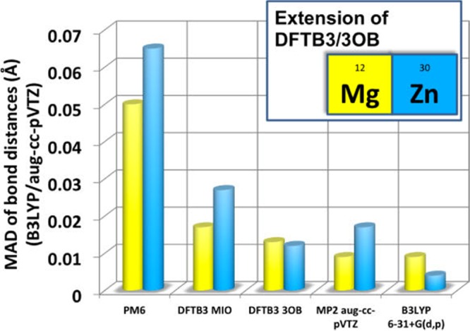
MADs of the bond distances of Mg²⁺ and Zn²⁺ test sets in ref (294) using the PM6, DFTB3/MIO, DFTB3/3OB, MP2/aug-cc-pVTZ, and B3LYP/6-31+G(d,p) methods where B3LYP/aug-cc-pVTZ is used as reference. Reprinted with permission from ref (294). Copyright 2014 American Chemical Society.

More recently, Gaus et al. parametrized the spin-polarized SCC-DFTB3 for Cu.²⁹⁵ Orbital angular momentum-dependent Hubbard U parameters (which equal twice the chemical hardness) and their charge derivatives were introduced to allow 3d and 4s orbitals to have different responses to charge density redistribution. The B3LYP/aug-cc-pVTZ level of theory was used to calculate the reference data. SCC-DFTB3 showed better performance than PM6 in predicting structural and energetic properties. However, it still gave less accurate results for charged ligands relative to neutral ones, which again may be due to the use of a minimal basis set.

Christensen et al. have incorporated the chemical-potential equilibration (CPE) model into the DFTB3 approach, along with an empirical dispersion correction that has two-body and three-body terms in 2015.²⁹⁶ The parameters for H, C, N, O, and S were determined for the new method (DFTB3/CPE-D3). CCSD(T) calculated interaction energies and DFT calculated dipole moments were used as targets for the fitting. The DFTB3/CPE-D3 approach showed good improvement in the description of charged species, while retaining its accuracy for describing neutral complexes, when compared to the DFTB3-D3 model. Generally, the DFTB3/CPE-D3 model showed better performance than the PM6-D3H4 method and the PBE-D3 method with a small basis set.

In 2012, Lukose et al. employed the SCC-DFTB method to study Zn, Cu, and Al-containing MOFs,²⁹⁷ in which they developed the Cu and Al parameters for the dispersion corrected SCC-DFTB method independently. The final results showed that the SCC-DFTB method reproduced both the structural properties and the absorption energies, when compared to benchmark DFT calculations. For example, the XRD patterns from experiment and DFT as well as DFTB optimized structures of the Cu-BTC MOF system are shown in Figure 8, which illustrates the good agreement between DFTB, DFT, and experiment. Because of the speed advantage, they proposed that it is possible to use the SCC-DFTB method to simulate MOF systems, which have unit cells of up to 10⁴ atoms.

Figure 8.

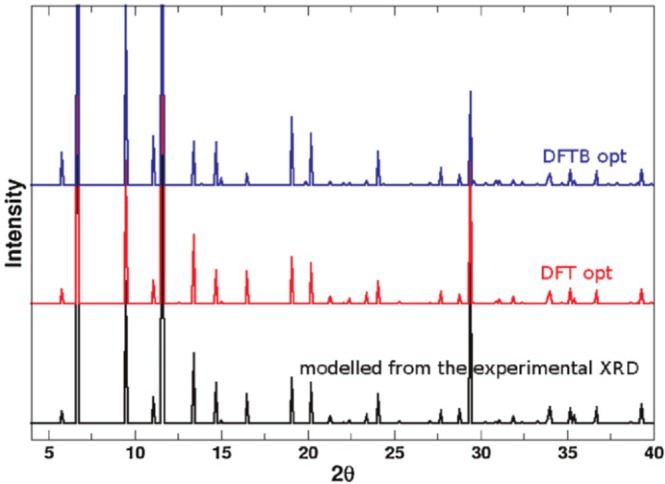
Simulated XRD patterns of the Cu-BTC MOF with the experimental unit cell parameters and optimized at the DFTB and DFT levels of theory. Reprinted with permission from ref (297). Copyright 2011 John Wiley and Sons.

2.5. Density Functional Theory Methods

The Thomas–Fermi model is considered to be the vanguard of modern DFT theory.^298,299 The modern DFT method was formalized in the theorems of Hohenberg–Kohn³⁰⁰ and then cast into the Kohn–Sham framework³⁰¹ in the 1960s. It represents the energy of molecules through the use of functionals of the electron density. There are various levels or rungs of DFT functionals: local density approximation (LDA), local spin density approximation (LSDA), generalized gradient approximation (GGA), nonseparable gradient approximation (NGA), Meta-GGA, meta-NGA, Hybrid GGA, Hybrid meta-GGA, and double hybrid methods, etc. Perdew and Schmidt systematically introduced different levels of approximations for the exchange-correlation energy based on their well-known “Jacob’s Ladder of DFT” concept (see Figure 9).³⁰² DFT has been shown to have good accuracy and has a speed advantage over the high-level post-HF methods and composite approaches, and is generally considered as the modern “work-horse” QM approach. For example, the total citation count for B3LYP³⁰³ and PBE,³⁰⁴ two widely used functionals, is over 130 000 (ca. 2016, from Google Scholar).

Figure 9.

Jacob’s ladder of density functional approximations. Any resemblance to the Tower of Babel is purely coincidental. Also shown are angels in the spherical approximation, ascending and descending. Users are free to choose the rungs appropriate to their accuracy requirements and computational resources. However, at present (ca. 2001), their safety can be guaranteed only on the two lowest rungs. Reprinted with permission from ref (302). Copyright 2001 American Institute of Physics Publishing LLC.

Because force fields derived on the basis of QM calculations usually make use of information derived from the Hessian matrix, which can be relatively expensive to compute, DFT has found a home in force field parametrization of TM-containing systems as it affords good accuracy at an affordable computational cost. Another advantage of DFT in modeling TM species is the incorporation of “static correlation”, giving DFT an improved ability to model multireference systems over its single referenced brethren based on the HF framework.¹³³ However, hybrid DFT functionals still have some single reference characteristics due to, in part, the use of exact exchange from HF calculation. Because of its nature, DFT computational errors are more randomly distributed than that observed in HF or post-HF methods.³⁰⁵ Moreover, DFT is usually not sensitive to the basis set used and converges quickly to the basis set limit.¹³¹

Overall, DFT is widely used to model TM-containing systems, but improved performance is not necessarily guaranteed if more sophisticated functionals are employed.³⁰⁶ Generally, the middle series TMs are hardest to model.³⁰⁷ If a DFT functional models one property well, this does not automatically mean that it will also perform similarly well on other properties.³⁰⁷ The accuracy of different functionals has also been shown to be system dependent for TM-containing species, and, overall, it is hard to identify one DFT functional that is accurate for a wide range of TM-containing systems.^308,309 In some work, it was found that nonhybrid DFT functionals offered more accurate results than hybrid ones,^310,311 while other work arrived at the opposite conclusion,^312−316 or no remarkable differences were found between the hybrid and nonhybrid functionals.³⁰⁶ Even though inclusion of a modest amount of HF exchange can improve results,^{309,313,315,317} too much HF exchange is generally not recommended.^313,318 For pure metals, the functionals that achieve the uniform gas limit work better than others.^190,191 According to several publications, the TPSS functional yielded the best results for modeling TM-containing systems.^{190,200,312,319−321}

There are very few DFT functionals specifically designed with TM-containing systems in mind. For example, the M06 functional developed by Zhao and Truhlar had TM properties included in its training set.³²² A recent double-hybrid DFT functional mPWPW91DH was designed to predict the electron response properties of TM-containing molecules.³²³ Recently, Yu et al. developed the gradient approximation for molecules (GAM) functional based on the NGA with reference database containing TM relevant energetic properties.³²⁴

Several benchmark studies regarding the performance of different DFT functionals in reproducing excitation energies, bond dissociation energies (BDEs), molecular geometries, HOFs, etc., of TM-containing systems have been reported. These results illustrate the advantages and disadvantages of various DFT functionals and offer insight into optimal methodological choices for particular problems containing TMs. In this active field, Truhlar and co-workers have performed an extensive series of benchmarks on DFT calculations on TM-containing systems.^{306,307,309,311,319,325} Wilson and co-workers have also performed a series of benchmarks on DFT functionals for TM species.^{313,314,317,326} Below, we briefly explore several examples.

2.5.1. Atomic Properties of Transition Metals

Using 60 different DFT functionals, Luo et al. in 2012 explored their ability to calculate the excitation energies of 4d TM atoms and their monovalent cations, as well as the IPs of the atoms.³⁰⁶ Analyses of fractional subshell occupancies and spin contamination were carried out, from which they sorted out the biases between s and d orbitals, and biases between low-spin and high-spin states. A general DFT functional should have little or no bias, rather than giving a satisfactory result simply due to error cancellation. The nonhybrid functionals have a tendency to overstabilize the 4d over the 5s orbitals, while HF exchange tends to decrease this bias. Local DFT functionals prefer low-spin states, while those with HF exchange tend to prefer the high-spin states. It was shown that there is no correlation between the general performance of a method and the amount of HF exchange included in the DFT functional. It was also observed that GGA and hybrid-GGA functionals outperform meta-GGA and hybrid meta-GGA methods, implying room for improvement of the meta-GGA and hybrid meta-GGA functionals.

Luo et al. have calculated excitation energies and IPs of 3d TM atoms covering 75 different DFT functionals in 2014.³⁰⁹ They note that studies on molecular systems enjoy some error cancellation effects that are not present in studies on atomic systems. It was again observed that no DFT functional performed well across a broad range of TMs. They discussed the notion that some amount of HF exchange is important for a balanced representation of the s and d orbitals, to accurately predict excitation energies and IPs.

2.5.2. Systems of Pure Metal or Those Containing Metal–Metal Bonds

Schultz et al. explored a series of TM dimers using 42 different DFT functionals in 2005.³¹¹ Overall, they observed that nonhybrid methods gave much better predictions than did hybrid functionals. For example, the PES and bond length of Cr₂ are shown in Figures 10 and 11, respectively. It was noted that inclusion of some HF exchange improved the accuracy for compounds containing “organic” and main group elements, but this was shown not to be the case for TM-containing systems. It was shown that even for the subset that does not have multireference character, similar trends were not found relative to modeling studies of organic molecules and TM dimers with respect to the accuracy of the different DFT functionals.

Figure 10.

Potential energy curve for Cr₂ computed with the mPW exchange functional and the KCIS correlation function using the following percentages of HF exchange: X = 0 (×), 1 (+), 2 (◇), 3 (□), 4 (△), 5 (○), 6 (*), 7 (−), and 8 (●), and experiment (solid line). Reprinted with permission from ref (311). Copyright 2005 American Chemical Society.

Figure 11.

Optimized bond lengths for the LSDA (△), GGA (×), hybrid GGA (□), meta GGA (◇), and hybrid meta GGA (○) with TZQ basis level and the experimental bond length (line) for Cr₂. Reprinted with permission from ref (311). Copyright 2005 American Chemical Society.

Zhao et al. examined 23 DFT functionals with two effective core basis sets (LANL2DZ and SDD) for modeling neutral and ionic Ag_n (n ≤ 4) clusters.¹⁹⁰ They found that, in general, functionals that achieve the homogeneous electron gas limit (e.g., PW91, PBE, P86, B95, TPSS, VSXC) outperformed the other functionals (e.g., the LYP and B97 series). For example, significant differences in the computed quantities for the Ag₃ and Ag₄ clusters were observed between the two groups. Therefore, care should be taken in choosing the appropriate functional for related studies. It was shown that the PBE1PBE (also known as the PBE0) functional predicted both the geometry and the energetic properties with good accuracy.

Paier et al. examined the ability of the B3LYP functional to predict the properties of solids (e.g., lattice parameters, bulk moduli, atomization energies, and reaction energies) in 2007.¹⁹¹ It was shown that the B3LYP functional gives comparable results for lattice constants as does the PBE functional but with different characteristics. B3LYP gave better predictions for systems with large energy gaps and strong electron localization, but showed reduced accuracy for metals (via an overestimation of the lattice constants due to an underestimation of the formation energies), when compared to the PBE functional. Moreover, the B3LYP functional predicts much poorer atomization energies than PBE0 and HSE03 (both hybrid functionals), which were developed to accurately model the uniform electron gas. They discussed that this was because of B3LYP’s weakness in attaining the uniform electron gas limit, reducing its ability to describe “free-electron-like” systems such as metals and semiconductors with small energy gaps. Lastly, it was shown the B3PW91 functional, which achieves the uniform electron gas limit, also offered obvious improvement in the reproduction of atomization energies over the B3LYP functional.

Gorelsky observed that the hybrid DFT functionals predict both the geometry and the energy poorly for the [V(C₅H₅)₂]Pn complex (with a V²⁺–V²⁺ bond and Pn represents pentalene; Figure 12 shows the complicated electronic structures of two V²⁺ ions), while GGA functionals gave better results.³¹⁰ The hybrid functionals were not recommended to study 3d TM complexes with weak or intermediate metal–metal bonds.

Figure 12.

Multiple electronic configurations that originate from the electronic interaction of two V^II ions. Reprinted with permission from ref (310). Copyright 2012 American Chemical Society.

To explore the bulk properties of 3d, 4d, 5d TM clusters, Janthon et al. used a number of different DFT functionals.³²⁵ The mean absolute percentage errors (MAPEs) for various DFT functionals regarding their ability to predict interatomic distances, cohesive energies, and bulk moduli are summarized in Figure 13. Hybrid functionals showed the best performance for calculating the interatomic distances, but poorly predict the cohesive energies and only show moderate performance in predicting the bulk moduli. It was proposed that this is due to the static correlation errors caused by inclusion of HF exchange.

Figure 13.

MAPEs for the interatomic distances, δ; cohesive energies, E_coh; and bulk moduli, B₀, of 27 transition metals with respect to experimental values extrapolated to 0 K and adjusted to remove zero-point vibrational contributions. MAPEs of δ has been multiplied by a factor of 10 for a better presentation. Data for LDA xc functionals, PBE, PW91, PBEsol, and RPBE are adapted from Janthon et al.³²⁷ Reprinted with permission from ref (325). Copyright 2012 American Chemical Society.

2.5.3. Geometries of Transition Metal-Containing Species

Bühl and Kabrede have explored the ability of multiple DFT functionals to predict the geometries of 32 3d TM complexes.³¹² They found that hybrid functionals modestly outperform the corresponding nonhybrid variants, while TPSS, a meta-GGA functional together with its hybrid variant, showed the best results.

Waller et al. have evaluated the performance of 15 DFT functionals in their ability to model the geometries of 19 4d TM complexes.³²⁸ They found that the GGA functionals all have bigger deviations than the corresponding hybrid ones. It was also shown that the overall deviation from experimental values did not decrease after adding zero-point vibrational corrections, which were calculated at the BP86/SDD level of theory, to the equilibrium bond lengths.

2.5.4. Energetic Properties of Transition Metal-Containing Species

Zhao and Truhlar assessed seven DFT functionals for their ability to predict reaction energies of 3d TM containing systems in 2006.³¹⁹ They found that M05 gave the best performance, B97-2 performed the best in predicting the binding energies, and TPSS works best for three TM dimers (Sc₂, Ni₂, and V₂), which have significant multireference characteristics.

Furche and Perdew explored the performance of several different DFT functionals for their ability to predict a series of properties (structures, dipole moments, bond energies, harmonic frequencies) of 3d TM-containing molecules in 2006.³²⁰ It was shown that BP86 (a GGA functional) and TPSS (a meta-GGA functional) yielded the best performance. They also proposed that the self-interaction error in one-electron and three-electron bonds appears to be the dominant error in the prediction of TM reaction energies when employing semilocal functionals.

Kasper et al. examined different properties of diatomic molecules of 3d TMs with H, N, C, O, S, F, Cl, and Br atoms employing five different DFT functionals in 2007.³⁰⁸ They found there is no universal functional and that the performance of different DFT functionals is system dependent. It was observed that hybrid DFT functionals usually underestimate the BDEs due to its preference for open-shell electronic structures, while GGA functionals usually overestimate them. It was also shown that the late TMs were better modeled using hybrid functionals, while the results of GGA functionals showed less preference. The hybrid DFT functionals also predict larger dipole moments than GGA ones, implying a less covalent bonding picture. The hybrid and GGA functionals differ significantly when modeling states with large spin contamination, hinting at the challenges faced by DFT in explaining the electronic structures of these systems.

In 2013, Zhang et al. explored how well 42 DFT functionals (in total 11 functional types including DFT-D) and the HF method reproduced select bond energies within 70 3d TM complexes.³⁰⁷ The meta-GGA, meta-NGA functionals showed improved performance over GGA and NGA methods, while there is no systematic improvement for the hybrid methods over nonhybrid ones. It was shown the TMs in the middle of the series (V, Cr, and Mn) are harder to model than the earlier and later ones. M–O and M–H bonds are hard to describe accurately, which may due to their multireference character. It was also demonstrated that DFT functionals, which yield good performance for the prediction of bond energies, may not be good for other properties.

Liu et al. used the catalytic properties of several 3d and 4d TMs for C–O bond dissociation as a benchmark set.³¹⁷ Calculations over eight DFT functionals were compared to values computed at the CCSD(T)/CBS level of theory. It was shown that reactions for earlier TMs have smaller activation energies and are more exothermic than the later ones, for both 3d and 4d species. Again, the percentage of HF exchange is crucial. The best results were obtained for 26% and 34% HF exchange 3d and 4d TM systems (see Figures 14 and 15), respectively. This interesting observation suggests that a higher percentage of HF exchange might be needed for systems with heavier metal ions.

Figure 14.

RMSDs of PBE versus percentage of HF exchange for 3d species. Reprinted with permission from ref (317). Copyright 2014 American Chemical Society.

Figure 15.

RMSDs of PBE versus percentage of HF exchange for 4d species. Reprinted with permission from ref (317). Copyright 2014 American Chemical Society.

Weymuth et al. benchmarked nine popular DFT functionals for the prediction of ligand dissociation energies in large TM complexes.³¹⁵ They found that for this end point, the performance of nonhybrid functionals was improved after incorporating some HF exchange. They also found that dispersion corrections decreased the performance of DFT functionals when predicting the dissociation energies of some ligands.

Riley and Merz investigated the accuracy of 12 DFT functionals covering GGA, hybrid-GGA, meta-GGA, and hybrid-meta-GGA functionals for 3d TM-containing molecules.³¹⁶ They used 94 experimental HOFs and 58 experimental IPs as reference data. They found that generally the hybrid DFT functionals performed better than the nonhybrid ones. The triple-ζ TZVP basis set generally outperformed the 6-31G** basis set. At least for the 6-31G** basis set, all of the DFT calculations give large HOF errors (6–12 kcal/mol bigger than the errors for organic molecules) when compared to experiment. The errors of the computed IPs are large as well (in the range of 0.85–1.20 eV), being about 3–4 times greater than the errors observed for organic molecules (in the range of 0.25–0.35 eV).

In subsequent work, Yang et al. explored the performance of the same 12 DFT functionals but with mixed basis sets (an ECP basis set with double-ζ - LANL2DZ for the TMs and 6-31+G** for the main group elements).³²¹ Interestingly, the mixed basis set strategy showed better performance than the single basis set strategy employed previously. Moreover, they found the GGA and meta-GGA functionals generally outperformed the hybrid functionals in predicting HOFs but showed less ability to predict IPs. The TPSSTPSS (with both exchange and correlation functionals labeled as TPSS) was able to predict both the HOFs and the IPs with reasonable accuracy. In related work from this group, Weaver et al. investigated 14 different DFT functionals, as well as the MP2, CCSD, CCSD(T), CASSCF, and CASPT2 methods for their ability to calculate the HOFs of zinc-containing molecules.²⁰⁰ The aug-cc-pVDZ and aug-cc-pVTZ basis sets were used in this research. TPSSTPSS and TPSSKCIS showed the best performance for the prediction of HOFs. It was shown that properly chosen DFT functionals yielded better performance than MP2 and CC methods.

Tekarli et al. have studied the HOFs of 19 3d TM complexes spanning over 44 different DFT functionals and compared them to experiment.³¹³ Overall, the top five best performing DFT functionals are all hybrid ones, clearly indicating that it is beneficial to include some amount of exact HF exchange. However, the hybrid functionals with more than 40% HF exchange performed poorly. CO-containing complexes proved to be very challenging for 42 out of the 44 functionals. The B97-1/cc-pVQZ level of theory showed outstanding performance, predicting HOFs ±1 kcal/mol with respect to composite methods based on high-level QM computations. The impact of the cc-pVTZ basis set versus cc-pVQZ was also explored, and it was shown that GGA and meta-GGA methods were less sensitive to basis set choice than the generalized gradient exchange (GGE), hybrid-GGA, and hybrid meta-GGA methods.

More recently, Jiang et al. have computed the HOFs of 193 3d TM-containing molecules using 13 DFT hybrid functionals and compared them to experiment.³²⁶ They observed that the B97-1 and mPW2-PLYP functionals gave the best performance (with MADs of 7.2 and 7.3 kcal/mol, respectively).

Shil et al. have benchmarked eight different “Minnesota” DFT functionals with 54 experimental HOFs and 47 experimental IPs of 3d TM complexes.³¹⁸ It was demonstrated that the performance of any given DFT functional decreased with an increase of the percentage of HF exchange. The meta-GGA method M06-L performed the best, while the hybrid metal-GGA method M06-HF, which use 100% HF exchange energy, gave the worst results. The unsigned average errors of HOFs for different functionals with respect to different ligating atoms are shown in Figures 16 and 17. From these figures, we see that the M06-HF has the largest errors, while the DFT functionals yield the biggest errors for CH₃ and CO coordinated TM complexes. Moreover, the largest errors were also found in the prediction of the HOFs of Fe complexes and the IPs of Ni complexes. This may be due to the multireference character afforded by partially filled d orbitals.

Figure 16.

Average unsigned heat of formation errors (kcal/mol) for the complete set of complexes, highlighting the performance of different M0X suite of functionals with LANL2DZ basis set, containing transition metals taken in the study of Shil et al.³¹⁸ Reprinted with permission from ref (318). Copyright 2013 American Chemical Society.

Figure 17.

Average unsigned heat of formation errors (kcal/mol) for different transition metal bonding partners treated in the study of Shil et al.³¹⁸ Reprinted with permission from ref (318). Copyright 2013 American Chemical Society.

Laury and Wilson investigated the HOFs of 30 4d TM-containing molecules with 22 different DFT functionals in 2013.³¹⁴ The MAD values are shown in Figure 18. This work found that the double hybrid DFT functionals B2GP-PLYP and mPW2-PLYP showed the best performance with MADs of 4.25 and 5.19 kcal/mol, respectively. The GGA functionals showed the largest errors, and are not recommended for computing thermochemical properties of 4d molecules. The hybrid-GGA methods showed good performance, with MADs of 6–10 kcal/mol. The mPW2-PLYP method with the cc-pVQZ-PP and effective core potential (ECP, for 4d metals) basis sets were proposed to be a good choice for calculating thermochemical properties of 4d TM-containing species.

Figure 18.

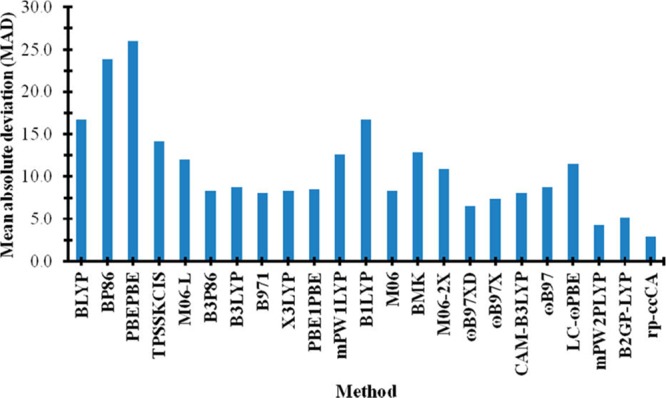
MADs of 22 DFT functionals and the rp-ccCA method for the HOFs of 30 molecules containing 4d TMs. Reprinted with permission from ref (314). Copyright 2013 American Chemical Society.

Grimmel et al. benchmarked a number of DFT functionals that range from LDA to double hybrid ones for predicting properties of Ln-containing molecules.³²⁹ 54 experimental HOFs of Ln species were employed as the reference data set. They proposed that 5.0 kcal/mol represented the “lanthanide chemical accuracy” based on the uncertainty of the experimental values. The results show that generally the nonhybrid functionals outperformed the hybrid ones. The TPSS functional yielded the best performance among the functionals they investigated.

2.6. Density Matrix Renormalization Group Method

The density matrix renormalization group (DMRG) method was proposed by White in the early 1990s.^330,331 It was developed on the basis of the renormalization (RG) method^332,333 and is an efficient method for modeling 1D systems and 2D systems. The number of degrees of freedom in Hilbert space for a many-body system grows rapidly as its size increases, but the DMRG method decreases the effective number of degrees of freedom. The computational complexity of the DMRG method is O(M²K⁴ + M³k³), where M represents the number of DMRG states and k indicates the number of one-particle orbitals.³³⁴ Generally, the DMRG method has a number of advantages over traditional QM methods. For example, the DMRG method follows both the size consistency and the variational theorem.³³⁵ Configuration interaction doubles (CID) and the quadratic configuration interaction singles doubles (QCISD) methods only obey the latter but not the former, while perturbation theory obeys the former but not the latter.³³⁵ Full CI obeys both features, but it has exponential scaling, while the DMRG method has polynomial scaling.³³⁶ The DMRG method includes the static correlation effect efficiently. For example, when compared to the CASSCF multireference method, the DMRG method can handle a much larger active space.³³⁶ However, the DMRG method is still computationally expensive when using larger basis sets to capture dynamic correlation effects.³³⁴ Even though the development of the DMRG method is still in its infancy, some progress has been made on TM-containing systems, and the method shows promise for future QM studies of TMs.

White and Noack performed the first application of the DMRG method on a 1D toy model.³³⁷ Nishino illustrated the application of the DMRG method to the interaction round a face (IRF) model.³³⁸ Fano et al. applied the DMRG method to cyclic polyene (CN)_n systems (with n up to 34) using the Pariser–Parr–Pople SE Hamiltonian.³³⁹ They explored the Hilbert space with a dimension of 5 × 10¹⁸ and showed that the DMRG method offered high accuracy, comparable to full CI and CC methods. However, they also pointed out that the DMRG method keeps a large number of matrixes when the interaction term relevant four orbitals are located in different blocks.³³⁹ White and Martin applied the DMRG method to ab initio quantum chemistry.³⁴⁰ They performed a study of H₂O with a standard Gaussian basis and obtained a total energy comparable to those obtained using CI and CC methods.³⁴⁰ Daul et al. illustrated the ability of the DMRG method to solve the full CI interaction problem. They applied the DMRG method to the paramagnetic HHeH molecule and discussed the basis set dependency, scaling issue, and also compared the DMRG method to other QM methods.³³⁵ Chan and Head-Gordon illustrated the formulation of the DMRG method in detail and tested its applications to water, ethane, and the nitrogen dimer systems.³³⁴ They found that the DMRG method offered excellent accuracy, especially when the static correlation is strong. However, they pointed out that it is computationally expensive for the DMRG method to evaluate the dynamic correlation effect with larger basis sets.³³⁴

Marti et al. applied the DMRG method to CoH, NiCO, and dinuclear Cu clusters in 2008.³⁴¹ Natural orbitals from CASSCF calculations instead of HF orbitals were used because they afforded better energies. They pointed out that the DMRG method could include more active orbitals than many QM methods, offering improved performance in modeling static correlation effects. They found that the total energy of the system decreases with an increase in the number of DMRG states, while the relative energy is easier to converge than the total energy. They also pointed out that one niche of the DMRG method in quantum chemistry is TM chemistry because it can handle much larger active spaces (bigger than 18 electrons and 18 orbitals) than the CASSCF method and qualitatively offers large-scale CASSCF wave functions and energies.³⁴¹

Kurashige and Yanai applied the DMRG method to study the PESs of the Cr dimer and isomerization of the [Cu₂O₂]²⁺ cluster in 2009.³⁴² They showed that the method offered excellent results for predicting these properties. Yan et al. studied the 2D kagome lattice in 2011 using the DMRG method, which proved its high accuracy for modeling the ground state.³⁴³ In 2013, Kurashige et al. applied the DMRG method to the Mn₄CaO₅ cluster in the PSII system.³⁴⁴ They considered more than 10⁸ quantum degrees of freedom, and the work marks the first treatment of the PSII system beyond the DFT single-electron picture.³⁴⁴ Sharma et al. explored the 2Fe-2S and 4Fe-4S clusters using the DMRG method in 2014.³⁴⁵ They found that the Heisenberg double exchange model largely underestimates the number of low-lying states, which are due to the neglect of iron d–d excitations, that are proposed to be important in these systems. Meanwhile, they found that the electronic energy levels are concentrated on the Fe–S clusters and vary on the vibrational fluctuation scale, offering an explanation of the wide existence of these clusters in nature.³⁴⁵

Recently, Olivares-Amaya et al. have presented benchmark results on a series of systems including the Cr dimer, Mn-oxo-salen, and Fe-porphine. They also offered a series of suggestions for doing DMRG calculations in practice.³⁴⁶ The BLOCK code, which was developed by Chan’s group, is now available in ORCA,³⁴⁷ Q-Chem,³⁴⁸ Molpro,³⁴⁹ and from Chan’s group.

2.7. Valence Bond Theory-Based Models

Besides the wave function-based QM methods and DFT, there are also VB-based QM methods available. Valence bond (VB) theory, which was proposed by Pauling, has played a key role in understanding chemical structure and reactivity.³⁵⁰ VB theory has two fundamental concepts: hybridization and resonance. It considers hybridization between different atomic orbitals while representing a molecule as a sum of its resonance structures with different weights. It offers a very intuitive perspective on chemical bonding and reactivity. For example, the hybridization concept is useful in determining molecular geometries (e.g., the VESPR theory). Even though MO theory is more widely used in contemporary computational chemistry, VB theory offers a more straightforward view of chemical bonds. VB theory uses localized hybrid orbitals (HOs) based on natural bond orbitals to model electronic structure, rather than the delocalized MOs obtained using the LCAO strategy employed in MO theory. However, these two perspectives on electronic structure are interchangeable via a unitary transformation of the density matrix of the natural localized molecular orbitals (NLMOs) to that of the delocalized canonical molecular orbitals (CMOs).³⁵¹ Hence, all of the physical properties calculated on the basis of NLMOs or CMOs should be identical, even though the two models afford different “localizations”. For simple cases, one Lewis structure is enough to obtain accurate results, while for more complicated systems, excellent results can be obtained using relevant resonance structures.^352−354

Examples of VB-based QM studies of metal ion-containing systems include the following: Goddard and co-workers developed the generalized VB (GVB) method³⁵⁵ and applied it to metal-containing molecules.³⁵⁶ Åqvist and Warshel reviewed the modeling of enzyme reactions (including those contain metals) and highlighted applications based on the empirical valence bond (EVB) method.³⁵⁷ Maupin, Voth, and co-workers studied the proton transfer mechanisms in human carbonic anhydrase II (HCAII)³⁵⁸ and its H64A mutant³⁵⁹ using the multistate empirical valence bond (MS-EVB) method. Wu et al. reviewed modern VB methods in 2011, and highlighted VB modeling on (CO)₄Fe(CH₂=CH₂).³⁶⁰

2.8. Basis Set Choices

Cundari et al. employed the B3LYP functional with the LANL and CEP-31G basis sets to study the HOFs of TM complexes in 2005.³⁶¹ It was shown that the former outperformed the latter in general. The results indicated that employing effective-core potentials for light elements (with atomic number less than 10) in the CEP-31G basis set was the major source of error. It was suggested that all electron basis sets be used for the main group elements when calculating the thermochemical properties of TM complexes.

In 2008, Williams and Wilson studied a set of group XI TM-containing molecules using MP2 and CCSD(T) methods with various cc-pVnZ-PP (where n = D, T, Q, and 5) basis sets on the metal ion, ligand, or both simultaneously.³⁶² The results showed that changing the ligand basis set but not the metal ion basis set has a much larger influence on the calculated geometry and dissociation energies than changing the metal ion basis set but not the ligand basis set. This indicated that the choice of basis set for the ligand is more important than that for the metal ion.

Xu and Truhlar have investigated the performance of HF-based effective core potentials when employing HF and DFT methods for 3d TM-containing systems.³⁶³ To evaluate the performance of different basis sets, 10 test cases were constructed, and the results were compared to the data obtained on the basis of a basis set incorporating the relativistic effect (NCBS-DK), and a basis set that did not consider relativistic effects (NCBS-NR). The all-electron def2-TZVP basis set was suggested to be used in relativistic and nonrelativistic DFT calculations for 3d TMs due to its excellent performance. These results also demonstrated that different DFT functionals affect the optimal choice of the ECP basis set.

2.9. Error Analysis

There have been few benchmark studies comparing accuracies of different kinds of QM methods and force fields for simulations of TM-containing systems. Related research efforts are encouraged because they can afford insights into the advantages and disadvantages of the relevant methods.

Amin and Truhlar have investigated the accuracy of 39 DFT functionals, the HF method, and 7 SE methods on their ability to predict the geometries, BDEs, and dipole moments of a series of zinc compounds.³⁶⁴ CCSD(T) and CCSD results were treated as the standard for comparison. They observed that all SE methods have 1.5–2.1 times bigger errors than the HF method, while DFT yields errors less than one-half of that of the HF method. The results demonstrated that DFT functionals for zinc compounds are consistent with what has been observed for main group compounds (functionals that offer good accuracy for organic molecules usually also yield good performance for zinc complexes). Moreover, it was shown that the performance of DFT functionals was improved via an admixture of exact exchange. In Lin and Wang’s research, they found that QM/MM simulation, with the SE method PM3 for the QM region (which contains three His residues, one zinc ion, and one ligand) and the AMBER ff03 force field for the MM region, gave larger structural distortions than the additive force field when compared to the XRD structure.

There are two main simulation issues nowadays: the accuracy of the potential and the extent of sampling. Some benchmark studies of protein systems showed encouraging results regarding unpolarized force fields. It was shown that some unpolarized force fields outperformed SE methods but were still inferior to DFT functionals in predicting the relative conformational energies of tetrapeptides³⁶⁵ and protein–ligand interactions.³⁰⁵ However, Faver et al. pointed out that it is still hard to predict the native structures of proteins on the basis of the current generation unpolarized force field models due to error accumulation.³⁶⁶ Even though QM methods offer considerable accuracy for simulating TM-containing systems and more QM simulations have been performed in recent years (e.g., the CPMD³⁶⁷ and nanoreactor³⁶⁸), classical models are still widely used due to their speed advantage, thereby accessing larger system sizes, longer simulation time scales, and broader conformational spaces, which are not accessible to QM-based simulations.¹⁴⁷ In the following, we briefly review popular classical models: the nonbonded, bonded, cationic dummy atom, combined, and polarizable models.

3. Classical Modeling of Metal Ions: The Nonbonded Model

3.1. Widely Used Potentials

There are two potentials widely employed to model the nonbonded interactions of ions: the 12-6 Lennard-Jones (LJ) potential³⁶⁹ and the Born–Mayer potential.³⁷⁰ The history of the evolution of these models is fascinating and involves some of the leading luminaries that laid the theoretical foundation to model intermolecular interactions.

In 1903, Mie proposed the Mie potential (see eq 21),³⁷¹ in which there are two parameters in the equation, n and m, representing the inverse-powers of the repulsion and attraction interactions, respectively.

21

It is a generalized form of the familiar Lennard-Jones expression. The modeling of periodic as well as charged systems was advanced in 1921 when Ewald described the so-called Ewald summation method to calculate the electrostatic energy inside periodic systems.³⁷² This approach and its variants are widely used in molecular simulations to calculate long-range electrostatic interactions.³⁷³

Lennard-Jones proposed the LJ equation (see eqs 22 and 23) to model the intermolecular interactions between argon in 1924,^374,375 where 5 was found as the best value for m while for n good agreement was found for all models when n > 9 with the best being n = . Hirschfelder et al. discovered that a 12-6 LJ equation could produce a good model for both helium and argon in 1938.³⁶⁹

22

23

London proposed the London equation (see eq 24) in 1930 to describe the magnitude of the dispersion interaction between two particles A and B using QM with second-order perturbation theory,³⁷⁶ in which the α_i and α_j are the dipole polarizabilities of particles i and j, while I_i and I_j are the first IPs of the particles.

24

Slater and Kirkwood proposed the Slater–Kirkwood formula (see eq 25) in 1931 and applied it to Ne, Ar, N₂, H₂, O₂, and CH₄.³⁷⁷ In their work, they used an exponential term to represent the repulsion interaction. In their formulation, ε is the mutual energy, v₀ is the highest quantum state electron number of the molecule, a₀ is the Bohr radius, E₀ is the ground-state energy of a hydrogen atom, while r_ij is the distance between two particles.

25

Buckingham proposed what came to be know as the Buckingham potential (see eq 26) in 1938 and applied it to gaseous He, Ne, and Ar.³⁷⁸ Similar to Slater and Kirkwood’s work, he used the exponential term to describe the repulsion interactions in the potential.

26

In 1918, Born and Lande proposed what came to be know as the Born–Lande equation (see eq 27) for calculating interactions inside ionic solids.³⁷⁹ As shown in eq 27, it uses a Born equation to describe the electrostatic potential (ESP), while an inverse-power term represents the repulsive interaction.

27

where N_A is Avogadro’s number, M is the Madelung constant, which depends on the lattice geometry, z⁺ and z^– are the charges for the positive and negative ions, respectively, e is the charge of a proton, ε₀ is the vacuum dielectric constant, while n is the Born exponent. By taking the derivative dU(r_ij)/r_ij = 0 when r_ij = r₀ (r₀ is the equilibrium distance between the two particles), one obtains:

28

29

Pauling estimated n in the Born–Lande equation over a range from 5 to 12 for different noble gas atoms and for the Cu⁺, Ag⁺, and Au⁺ ions.³⁸⁰ In 1932, Born and Mayer proposed the Born–Mayer potential (see eqs 30 and 31; eq 31 was obtained similar to eq 29 based on eq 27) where they used an exponential term e^–r/ρ instead of the inverse-power term r^–n to represent the repulsion interaction.³⁷⁰ ρ is a constant that depends on crystal compressibility, and a value of 30 pm gave a good description for the alkali metal halides.³⁷⁰ Finally, r_i and r_j are the ionic radii of the ions, while A_ij was a factor determined by Pauling, generally set to 1.00 for a cation–anion pair, 0.75 for an anion–anion pair, and 1.25 for a cation–cation pair.³⁷⁰

30

31

In the subsequent year, Mayer added a r^–6 (representing dipole–dipole interactions) and a r^–8 (representing quadruple–dipole interactions) dispersion term into the Born–Mayer potential (see eq 32),³⁸¹ where the dispersion parameters were estimated from the formula given by Margenau.³⁸² The potential showed improvement for the CsCl lattice type (i.e., the CsCl, CsBr, and CsI ionic compounds). Huggins and Mayer determined the ionic radii (which were used to determine the strength of the repulsion term) for five alkali metal ions (Li⁺, Na⁺, K⁺, Rb⁺, and Cs⁺) and four halide ions (F^–, Cl^–, Br^–, and I^–).³⁸³ On the basis of these values, experimental lattice constants were reproduced for 20 alkali metal–halide ionic solids.

32

Tosi and Fumi revisited ionic compounds using two different potentials (i.e., using the exponent and inverse-power as the repulsion terms, respectively) and determined the crystal radii of NaCl-type alkali halides in 1964.^384,385

3.2. 12-6 Lennard-Jones Potential

3.2.1. Functional Format

The popular 12-6 LJ potential approximates the repulsion interaction, which is best modeled via exponential decay along with the particle distance (i.e., as described by the Buckingham potential and Born–Mayer potential; see eqs 26 and 30).³⁸⁶ However, when applying these potentials to a molecular structure where two particles are too close with each other, the Buckingham or Born–Mayer potential can yield a negative interaction energy, while the 12-6 LJ potential prevents this from happening. Moreover, the 12-6 LJ potential is calculated 4 times faster than the Buckingham potential.³⁸⁷ Another consideration is the 12-6 LJ potential needs less parametrization work than the Buckingham potential (two versus three parameters, respectively), which also supports its wide utilization in molecular simulations. Furthermore, the 12-6 LJ potential yields accuracy similar to that of the Buckingham potential after careful parametrization when used in a molecular force field. For example, Lifson and Warshel found that applying the Coulombic equation and a Urey–Bradley-type force field plus the 12-6 LJ potential in the CFF formulation offered improvement in modeling the intermolecular interactions in cycloalkane and n-alkane (with n = 5–12) systems in 1968.³⁸⁸ Jorgensen also found that a 12-6-3 potential gave almost the same accuracy as the exponential function to describe the short-range interactions between two water molecules in 1979.³⁸⁹

The 12-6 nonbonded potential for ions represents ionic interactions between a metal ion and the surrounding particles as a sum of the electrostatic and VDW terms. This model closely reproduces the situation for monovalent ions that have low electronegativities (e.g., alkali metal ions). However, the quality of this representation degrades for systems containing divalent or highly charged ions, where the POL and CT effects are significant.^390,391

The form of the 12-6 LJ nonbonded potential, between particles i and j, is given in eq 33. Three different forms are in common usage, and each is given in eq 33. Q_i and Q_j are the partial charges on the two particles. In the nonbonded model, the metal ion is generally modeled using an integer partial charge equal to its oxidation state. The only parameters that need to be determined are A_ij and B_ij, R_min,ij and ε_ij, or σ_min,ij and ε_ij depending on the form of the equation.

Figure 19 visualizes the differences and physical meaning of the R_min,ij and ε_ij, and σ_ij and ε_ij forms, which are in common usage. R_min,ij is the distance at which the LJ potential has its minimum value, while σ_ij is the distance at which the LJ potential is equal to zero. ε_ij is the well depth of the LJ potential curve, representing the VDW interaction strength between the two particles. If we have N atom types employed in a force field, there will be unique atom pair types. All forms of the LJ potentials have two parameters (A_ij and B_ij, R_min,ij and ε_ij, or σ_ij and ε_ij) for each atom type pair, which leads to N(N + 1) LJ parameters that need to be parametrized. This represents a tremendous parametrization effort; hence, a number of combining (or mixing) rules were introduced to reduce the overall parameter space. By obtaining the A_ii/B_ii/R_min,ii/σ_ii/ε_ii and A_jj/B_jj/R_min,jj/σ_jj/ε_jj values, first the pairwise A_ij/B_ij/R_min,ij/σ_ij/ε_ij parameters are obtained from the former two using an appropriate combining rule. This decreases the number of parameters to 2N. Popular force fields such as AMBER,^392−400 CHARMM,^401−406 OPLS-AA,^407−411 etc., treat several different atom types of the same element with identical LJ parameters, further decreasing the parametrization effort.

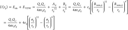33

Figure 19.

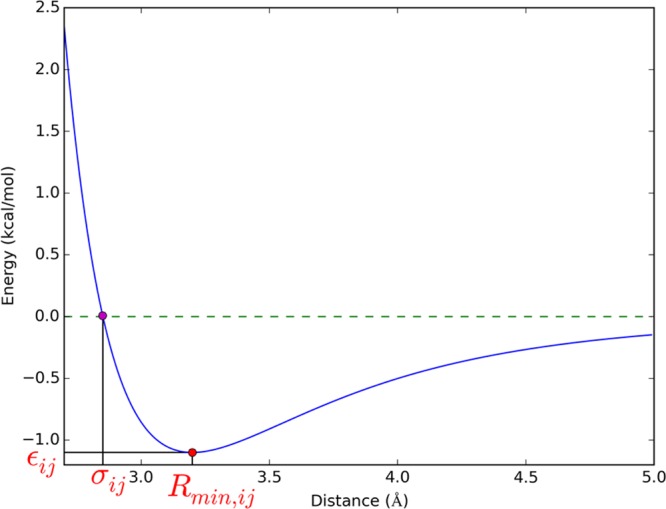
Representation of R_min,ij, σ_ij, and ε_ij in a 12-6 LJ equation. Here, we illustrate the LJ potential between two particles, which have the same R_min,i (1.6 Å) and ε_i (1.1 kcal/mol) values.

Below we summarize some of the most widely used combining rules.

(1) For A_ij and B_ij terms, the geometric combining rule is generally used:

34

(2) For R_min,ij and σ_min,ij, the arithmetic (Lorentz), geometric (Good–Hope), and sixth power (Waldman–Hagler) combining rules are used extensively.

Lorentz combining rule:

35

Good–Hope combining rule:

36

Waldman–Hagler combining rule:

37

(3) For ε_ij, the geometric (Berthelot) and sixth power (Waldman–Hagler) combining rules are widely used.

Berthelot combining rule:

38

Waldman–Hagler combining rule:

39

Note: For clarity, we will use the following nomenclature throughout.

40

41

42

43

44

The Lorentz combining rule (or arithmetic combining rule) depends on the hard sphere assumption, in which particles are treated as rigid balls. The optimal distance of the VDW interaction is the sum of VDW radii of the particles i and j. The geometric combining rule relies on a “soft sphere” assumption. In eq 45, we exemplify this rule for the determination of ε_ij: the smaller of ε_ii and ε_jj has a bigger weight in the determination of the final value of ε_ij.

45

3.2.2. Parametrization Strategies

The parameters of ions are usually determined by reproducing one or several theoretical/experimental end points using force field (FF) calculations either through single point energy calculations or via MC⁴¹² or MD⁴¹³ simulations. Target values used for model construction and validation can be classified as thermodynamic quantities (e.g., interaction energy, calculated potential energy surface (PES), HFE, hydration entropy, crystal lattice energy (LE), etc.), structural properties (e.g., QM calculated equilibrium distance, ion–oxygen distance of the first solvation shell (IOD), CNs of the first solvation shell, crystal lattice constant (LC), etc.), and kinetic or dynamic properties (e.g., exchange rate of first solvation shell water, diffusion coefficient (DC), etc.). From the phase state point of view, the parametrization end points can be classified as solid-state properties (LC, LE, etc.), liquid phase properties (HFE, solvation entropy, IOD, DC, mean residence time of first solvation shell (MRT), activity coefficient (AC), etc.), gas-phase properties (interaction energy of monohydrates, PES, etc.), and interface properties (osmotic pressure, etc.). From another perspective, the reference properties can be classified as single ion properties (HFE, IOD, CN, etc.), ion-pair properties (AC, Kirkwood–Buff integral (KBI), etc.), along with mixed system properties (osmotic pressure of a biomolecular system, etc.). Typical ion parametrization efforts fit two or more properties for a single-ion at a time and then afterward test their transferability to other systems or properties. For example, if an ion model was parametrized in aqueous solution using a specific water model, its transferability to other water models, with other ions (to explore ion-pair properties), in combination with other atom types in a mixed system (such as a biological system) would ultimately need to be addressed to fully validate the model.

In the pioneering efforts on ion parametrization, when computational resources were at a premium and free-energy simulation methods were not widely available, researchers usually parametrized the potential by reproducing QM-derived interaction energies and equilibrium distances or by fitting the potential to a simulated PES obtained from QM calculations on the monohydrates. However, potentials derived in this way had errors arising from the neglect of three-body and higher order effects. This causes an overestimation of the interaction energy between the solvated ion and water and then, ultimately, the ion’s HFE. This error increases dramatically for the divalent and highly charged metal ions, for which the CN values predicted from molecular simulations based on the conventional pair potential are generally higher than the experimentally determined CN values. Work has been done to add the three-body term and higher order terms into the function, and remarkable progress has been made in this area.^414−417 However, the computational complexity and parametrization effort increase considerably at the same time. Hence, work focusing on adding these effects into a pair potential, yielding an effective pair potential, has been the preferred approach. This potential can be parametrized in multiple different ways, such as fitting to a QM-based effective potential, or parametrizing it directly to reproduce experimental results.

3.3. Early Studies

The modern computer was invented in the last century; for example, the ENIAC (electronic numerical integrator and computer) was announced in 1946.⁴¹⁸ In the 1960s, supercomputers began to become available to investigators at major universities and institutes. Concomitant with hardware developments, QM methodologies and software were becoming widely available, allowing force fields to be parametrized on the basis of accurate QM calculations, while ever more sophisticated and realistic simulation of ionic compounds, aqueous solutions, proteins, etc., began to regularly appear in the literature.

3.3.1. Studies Based on the Monte Carlo Method

The MC method analyzes a system by generating a structural ensemble whose energy follows a Boltzmann distribution. The modern MC method was proposed by Metropolis and Ulam in 1949.⁴¹² This paper was then followed by a number of applications on molecular or molecular-like simulations. Rosenbluth and Rosenbluth performed a MC simulation for a three-dimensional system with a hard sphere potential and a two-dimensional system with a LJ potential in 1954.⁴¹⁹ Wood and Parker performed a MC simulation of an Ar gas system using a 12-6 LJ potential in 1957.⁴²⁰ Several properties such as the radial distribution function (RDF), excess internal energy, compressibility factor, etc., were obtained, and a liquid–solid transformation was observed during the simulation. The simulated results agreed with one set of experimental results but disagreed with another.⁴²⁰ Barker simulated proton–electron plasma at various temperatures and densities using the MC method in 1965.⁴²¹ In these simulations, he employed a Columbic potential coupled with the Ewald sum method to estimate long-range electrostatic interactions during the simulation. The results supported the usefulness of the MC method. Woodcock and Singer carried out a MC simulation for solid KCl using a Born–Mayer–Huggins potential in 1971.⁴²² They calculated a series of properties such as pressure, entropy, internal energy, etc., for different volumes, temperatures, and pressures. The results showed good agreement with experimental results. Furthermore, some experimentally inaccessible data (such as the contribution of different energy terms, properties at extreme temperatures/pressures, etc.) were obtained using these simulations. They found that the r^–8 (dipole–quadrupole) term is only responsible for −0.5% of the internal energy along their simulation, and hence could be safely neglected during the simulation.

Clementi and co-workers fit a series of potentials based on QM calculations and performed a range of related MC or MD simulations for ion-containing systems (e.g., ionic solution,^423−429 ion-nucleic acid,^430−434 and ion-transmembrane channel^435−438 systems) in the 1970s and 1980s.

3.3.2. Studies Based on Molecular Dynamics Simulation

The MD simulation method integrates Newton equations of motion to simulate a system by propagating the positions, velocities, and accelerations of particles as a function of time. MD not only provides thermodynamic and structural properties akin to MC simulations, but it can also directly simulate time-related properties. Alder and Wainwright reported the first MD simulation for a hard sphere system in 1957,⁴¹³ and they proposed a propagation algorithm for MD simulations in a later work.⁴³⁹ Gibson et al. described a MD simulation exploring the mechanism of damage of solid Cu using a Born–Mayer potential in 1960.⁴⁴⁰ Later, Rahman simulated liquid Ar using the MD method in 1964.⁴⁴¹ Periodic boundary conditions combined with a truncated LJ equation were used to carry out the simulation. The simulated pair-correlation function was in good agreement with experiment, while the calculated self-diffusion constant was 15% smaller than the experimental value. Woodcock performed the first ionic compound MD simulation (on LiCl, NaCl, and KCl compounds) in 1971, again using a Born–Mayer potential.⁴⁴² The potential parameters were from Tosi and Fumi’s previous work,³⁸⁴ while the Ewald method was used to model the electrostatic interactions. Various properties such as the specific heat capacity, entropy, and diffusion coefficient, etc., were obtained for the three liquid alkali metal halides at 1273 K and showed good agreement with experimental results.

Rahman and Stillinger performed the first simulation of liquid water system in 1971, in which they used a five-site water model with a tetrahedral configuration (so-called the ST2 water model).⁴⁴³ The two-body potential was parametrized to reproduce the water dimer interaction energy from ab initio QM calculation. Both structural (e.g., pair-correlation functions, CNs, distribution functions, etc.) and kinetic properties (such as center-of-mass motion mean-square displacement, autocorrelation functions of the velocity, dipole relaxation function, etc.) were calculated, and good agreement was obtained when compared to experimental results.⁴⁴³

Heinzinger and Vogel performed the first MD simulation of an ionic solution system (LiCl in water) in 1974.⁴⁴⁴ In their work, they used the ST2 water model proposed by Rahman and Stillinger.⁴⁴³ The 12-6 LJ nonbonded model was used for the ions, and the LJ parameters were obtained directly from the LJ parameters for He and Ar (as they are isoelectronic with Li⁺ and Cl^– ions, respectively) determined by Hogervorst⁴⁴⁵ (where the parameters were obtained by parametrizing against experimental viscosity values). The combining rules were taken from Kong,⁴⁴⁶ while a switching function was utilized for the evaluation of the Columbic terms. The simulated structure of the first hydration shell showed good agreement with experimental XRD and neutron diffraction data, and the simulation was able to predict the faster rotation of the first solvation shell water molecules of the Li⁺ ion (relative to other water molecules in the system), in agreement with nuclear magnetic resonance (NMR) results.

Jorgensen and co-workers parametrized the LJ potential for Na⁺ using the transferable intermolecular potential function (TIPS) format,⁴⁴⁷ and the Li⁺, Na⁺, F^–, and Cl^– ions for the TIP4P water model based on QM calculated energetic and structural information in the 1980s.⁴⁴⁸

Bounds parametrized Li⁺, Na⁺, K⁺, Ca²⁺, and Ni²⁺ using QM calculations and simulated them with the TIP4P water model of Jorgensen and co-workers⁴⁴⁹ via MD simulations in 1985.⁴⁵⁰ Ca²⁺/H₂O and Ni²⁺/H₂O potentials were derived from ab initio SCF calculations.⁴⁵⁰ Exp-4-6-1 and exp-1 formatted functions were used for the ion–oxygen and ion–hydrogen interactions, respectively. A higher CN for Ni²⁺ (as high as 8) was predicted from the simulation, which is greater than the experimentally determined CN of 6. High pressure affected the second-coordination shell of Cl^–, while high temperature and pressure showed little effect on the structure of Ca²⁺ in aqueous solution.

In 1986, Teleman and Ahlstrom simulated the Ca²⁺ EDTA complex and the Ca²⁺-aqueous system based on the VDW parameters derived from the Kirkwood–Slater formula.⁴⁵¹ The simulated CN of Ca²⁺ in both water and EDTA is ∼7. The observed structural properties were “plausible”, while the simulated dynamics were deemed “fast” relative to experiment.

It was observed in the late 1980s that there are considerable errors when applying the conventional pair potential to calculate HFEs for ions. For example, Migliore et al. calculated the HFEs of the Li⁺, Na⁺, K⁺, F^–, and Cl^– ions on the basis of the parameters fitted to the configuration interaction (CI) QM calculations. They found that the errors in the simulated HFEs are considerable, ranging from −30% for Cl^– to 21% for Na⁺ when compared to experimental values.⁴⁵² Straatsma and Berendsen studied the HFEs of Na⁺, K⁺, Ca²⁺, F^–, Cl^–, and Br^– ions using the thermodynamic integration (TI) approach, and they observed that the simulated HFEs of these ions (except for the Ca²⁺ ion) were too negative when compared to experiment.⁴⁵³ These results indicated that many-body effects are important and that a potential fitted from a monohydrate in the gas phase does not have good transferability to the liquid phase.

3.3.3. Many-Body Effects

As described above, the conventional pair potential, when fitted to QM calculated results on monohydrates in the gas phase, yields a notable overestimation of the ion–water interaction in the aqueous phase, in part due to the neglect of many-body effects. For starters, the first, second, third, and nth water binding energies to the metal ion tend to decrease. The QM fitted potential generally only considers the first water molecule, which will lead to an overestimation of the effective potential for ion–water interactions in aqueous systems. This leads to higher HFE values and may cause an increase in CN over that observed experimentally. This error can be decreased using error-canceling strategies, for example, using small basis sets, which underestimate the interaction energy of the monohydrates.

Another concern has to do with the M^q+–H₂O system becoming the M^(q–1)+–H₂O⁺ species at long distances, because the qth IP of the metal ion is higher than the first IP of the water molecule.⁴⁵⁴ A positive charge on both the ion and water will cause repulsion between them. Marcos et al. proposed that for Zn(H₂O)²⁺, the crossing of the two ¹A₁ symmetry states (Zn²⁺–H₂O and Zn⁺–H₂O⁺) appears at 4.5 Å.⁴⁵⁵ For Be(H₂O)²⁺, Corongiu and Clementi found its crossing occurs at ∼9 bohr (∼5.3 Å). Curtiss et al. found that the crossing distances for Fe(H₂O)²⁺ and Fe(H₂O)³⁺ were >6 Å and “close to” 1.852 Å, respectively.⁴⁵⁶ However, in an aqueous system, the other n–1 water molecules in the first solvation shell (assuming there are n water molecules in the first solvation shell) will stabilize the charge on the ion, preventing the formation of the M(H₂O)_n^(q–1)+–H₂O⁺ species at long-range. Using a restricted Hartree–Fock (RHF) method, the M^q+–H₂O electronic configuration can be retained at long-range (even if this is in fact not natural) to obtain the PES, but this kind of strategy may fail when using correlated methods.⁴⁵⁴

Using some fitting strategies (e.g., using small basis sets), the error can be decreased to some extent; however, the HFE and CN values may still be overestimated for some ion-aqueous systems, especially for the highly charged ions, for which the many-body effect is significant. There are several ways to address the many-body problem: (A) adding the many-body terms; (B) using an effective potential; and (C) using a combined model for the hydrated complex (discussed in section 5.2).

3.4. Many-Body Potentials

In 1980, Clementi et al. studied the nonadditivity of the Li(H₂O)₂⁺ system using QM calculations after which an atomic charge-induced bond dipole term and a short-range correction term were added to the pair potential to represent the three-body effect.⁴⁵⁷ Overall, they found the three-body term was 10–15% of the total interaction. On the basis of this three-body potential, Corongiu et al. calculated the HFE value of Li⁺ using MC simulations with the free-energy perturbation (FEP) method and obtained a HFE for the Li⁺ ion of −114 ± 8 kcal/mol, in good agreement with two different experimental values (−118 or −123 kcal/mol).⁴⁵⁸ However, using a conventional pair potential, which only considered the two-body effect, they overestimated the HFE value (−142 ± 2 kcal/mol).

As compared to the monovalent ions, the three-body effect would be expected to be even more significant for highly charged ions in aqueous solution. Bounds simulated Ni²⁺ in aqueous solution using an ab initio pair potential and predicted a higher CN (8 versus 6 from experiment) and an IOD value larger than experiment (2.17 Å versus 2.07 Å),⁴⁵⁰ and González-LaFont et al. predicted a higher CN value for the Fe²⁺ ion (8 versus 6) also using an ab initio pair potential.⁴⁵⁹

Natália et al. studied Ni²⁺ in aqueous solution using a conventional two-body potential and a potential with a three-body term.⁴⁶⁰ The conventional two-body potential overestimated the CN, giving a value of 8 instead of 6 and an IOD of 2.09 Å rather than 2.07 Å. The potential with the three-body term correctly simulated the CN and IOD values, but still overestimated the hydration enthalpy by ∼158 kcal/mol. Nonetheless, this was a smaller extent than the value given by the two-body potential (which overestimated the value by ∼295 kcal/mol). They proposed that further improvement could be achieved via addition of a short-range correction term and through the use of the Ewald summation method instead of a truncated potential.

Curtiss et al. have also investigated the Fe²⁺ and Fe³⁺ ions in aqueous solution using a pair potential fitted from ab initio calculations.⁴⁵⁶ Higher CN and longer IOD values were simulated for the Fe²⁺ and Fe³⁺ ions as well. Subsequently, they parametrized an empirical pair potential that accurately reproduced the CN values of the Fe²⁺ and Fe³⁺ ions.⁴⁵⁶

Yamaguchi et al. simulated BeCl₂ in aqueous solution based on an ab initio pair potential and obtained a CN value for the Be²⁺ ion of 6, which is inconsistent with experimental XRD data, which gave a CN of 4.⁴⁶¹ Through an addition of a three-body term into the potential, Probst et al. were able to reproduce the CN of the Be²⁺ ion correctly.⁴¹⁴

Cordeiro and Gomes have examined three-body, four-body, and higher order terms for Cu(H₂O)_n²⁺, where n ≤ 8.⁴¹⁵ During these studies, they found that three-body terms, which contribute repulsive interactions to the pair potential, are non-negligible. The potential with a three-body term correctly simulated the CN value (as 6) and offered improvement over the conventional two-body pair potential based on ab initio calculations (which gave a CN of 8). They also found a rapid convergence of the many-body expansion in that the four-body and higher order terms are much smaller than the three-body term. Rode and Islam found similar issues using an ab initio pair potential when they simulated the Cu²⁺ ion in aqueous solution.⁴¹⁶ To tackle these issues, they proposed a three-body term they called the nearest neighbor ligands correction (NNLC) that affected the first solvation shell. This strategy was not only able to reproduce the experimental CN, but it also reduces the potential parametrization burden and simulation time when compared to a potential with more typical three-body terms.

To gain deeper insights into the Cu²⁺ aqueous system, Cordeiro and Gomes reinvestigated it through a comparison of several different potentials.⁴¹⁷ These potentials included the conventional two-body fitted ab initio potential, the effective two-body ab initio potential (fitted from the interaction of Cu²⁺ with its first solvation shell waters), the conventional potential with a three-body term, and the effective potential with a three-body term. They found that both the effective pair potential and the three-body term decreased the average interaction energy between the ion and surrounding water molecules. They also found that the conventional potential overestimated the interaction energy by ∼30% over the effective potential in the first solvation shell, while they were nearly identical outside the first solvation shell. However, the conventional and effective two-body potentials overestimated the CN values as 8–9 and 8, respectively. Both the conventional potential with a three-body term and an effective potential with a three-body term offered improvement with the latter better describing the energetics of the system. Furthermore, they noted that in the three-body term, the ion–water–water term dominates the water–water–water term.

3.5. Effective Two-Body Potentials

There are two different ways to incorporate many-body effects into effective two-body potentials. One is based on fitting to QM-derived data, and the other involves fitting the potential directly to experimental HFE, IOD, etc., values as demonstrated by Aqvist.⁴⁶² The methods based on fitting to QM data may still not reproduce the HFE or IOD values accurately due because the reference QM model they fitted to may still only have finite accuracy, with the resultant error propagating with the increasing size of the simulated system. Hence, people prefer to use the latter method in parametrization efforts because it accurately reproduces thermodynamic, structural, or both properties simultaneously.

3.5.1. Quantum Mechanics-Based Parameters

There are different approaches to fit effective two-body potentials based on QM data, for example, (1) fitting the potential between an ion and water within a implicit solvation model, as proposed by Floris et al.,⁴⁶³ (2) fitting the potential to reproduce the average interaction between an ion and its first solvation layer, as proposed by Cordeiro et al.,⁴¹⁷ and (3) fitting the potential to reproduce the PES between the ion, which has n–1 water molecules bound to it (where n is the CN value) with fixed geometry, and the last water, as proposed by Periole et al.⁴⁶⁴ The accuracy of the first method depends on the accuracy of the implicit solvation model, while for the second and third approaches, errors associated with only considering the first solvation shell can reduce their accuracy.

3.5.1.1. Effective Potential Based on Implicit Solvation Model

Floris et al. proposed a QM method to obtain the effective pair potential, which considers many-body effects implicitly.⁴⁶³ They applied their methodology to Fe²⁺ and Fe³⁺ aqueous systems initially and were able to reproduce the experimental CNs.⁴⁶³

46

As given in eq 46, the interaction energy U_AB of two solutes in solvent can be obtained on the basis of QM calculations, where is the Hamiltonian of the solute in vacuo while ψ is the wave function for the solute in solution, which was modeled using the polarizable continuum model (PCM). They found that, for Fe²⁺ ion, the conventional pair potential fitted using the dihydrate complex in vacuo yielded a lower binding energy by ∼15 kcal/mol than the conventional pair potential fitted from the monohydrate in vacuo. Using their approach with an effective pair potential fitted using both the monohydrate and the dihydrate data simultaneously further decreased the binding free energy by ∼4 kcal/mol. However, this method depends on the accuracy of the implicit solvation model itself and the parameters employed in the solvation model. The broad range of available solvation models has been extensively reviewed by others.⁴⁶⁵ In the work of Floris et al., they used the U_WMW = 2U_MW + U_WW relationship (where M = metal and W = water) to determine the ionic radii for Fe²⁺ and Fe³⁺ ions.⁴⁶³ Finally, they fitted their potential based on a range of ion–water structures and the SPC water model. The resultant potential reproduced the experimental CNs for the Fe²⁺ and Fe³⁺ ions (as 6) and the octahedral geometry of the first solvation shell.

Subsequently, Floris et al. have used their approach to study the aqueous hydration of a range of ions including Li⁺, Be²⁺, Mg²⁺, Ca²⁺, Ni²⁺, Zn²⁺, Al³⁺, and Ln³⁺.^454,466,467 The results obtained further confirmed that their approach offers improvements over the conventional pair potential.

D’Angelo, Chillemi, and co-workers studied Co²⁺, Zn²⁺, and Ni²⁺ in aqueous solution using an effective pair potential based on the method developed by Floris et al.^468,469 The PES was evaluated using restricted-open-shell-Hartree–Fock (ROHF) calculations coupled with the PCM solvent model. Even with the complicated potential equation they used (Exp-1-4-6-8-12 potential for the ion-oxygen and a 1-4-6-8-12 potential for ion-hydrogen; see eq 47), MD simulation of Zn²⁺ in water predicted a more asymmetric and a sharp first peak in the metal–oxygen RDF when compared to the EXAFS results. They also used this method to investigate Hg²⁺, trivalent metal ions in the lanthanide series (Ln³⁺), and trivalent metal ions in the actinide series (An³⁺) in aqueous solution and obtained useful insights.^470−475 Besides aqueous solution, they also utilized this method to explore Zn²⁺ and Hg²⁺ in methanol.^476,477 While their approach proved powerful, it has some issues affecting its usability; because of its complicated form, the number of parameters will increase dramatically in mixed systems such as proteins and nucleic acids, reducing its broad applicability.

47

3.5.1.2. PES Scanning Method

Pang et al. parametrized the Fe²⁺ ion with a 12-6 LJ potential for a nonheme site.⁴⁷⁸ The parameters were derived on the basis of the QM PESs between Fe²⁺ and the ligating ligands (two His residues, one Asp residue, one water, and one α-ketoglutarate ligand). They applied a weak harmonic restraint to favor the monodentate Asp binding mode over the bidentate mode frequently preferred by the 12-6 LJ nonbonded model.

3.5.1.3. SLEF Model

Wu et al. have developed the nonbonded short–long effective function (SLEF) model and parametrized it for zinc-containing proteins via reproduction of QM/MM-derived forces for zinc metalloenzymes with different binding modes (with CNs equal to 5, 6, and 7).⁴⁷⁹ The SLEF model, instead of the standard Columbic formula, was used to represent the electrostatic interactions between the Zn²⁺ ion and the surrounding particles (see eq 48). The short-range part decays exponentially, while the long-range part contains a term similar to a DFT dispersion correction damping function. As shown in Figure 20, the PES between the zinc ion and the TIP3P water model shows that SLEF strengthens the short-range interactions (from 1.5 to 2.0 Å) and weakens the midrange (from 2.5 to 4.5 Å) interactions, while retaining the strength of the long-range (beyond 4.5 Å) interactions, relative to the standard Columbic model. This behavior implicitly incorporates POL and CT effects into the modeling of the metal ion. Exploratory MD simulations were carried out for Zn²⁺ metalloenzymes with CN values of 5, 6, or 7, and comparisons were made between SLEF and standard 12-6 LJ models. The SLEF model showed improved performance and was able to reproduce different binding modes as shown by QM/MM MD and experimental results.

48

Figure 20.

Illustration of the difference between SLEF and the conventional 1/r Coulomb function in describing charge interactions between Zn²⁺ and the oxygen of TIP3P water: (A) energy and (B) force. The parameters in the SLEF1 force field were employed. Reprinted with permission from ref (479). Copyright 2011 American Chemical Society.

Afterward, Gong et al. developed a second-generation approach (SLEF2, see eq 49) where they optimized the parameters (α, β, γ, λ, and R_Zn) on the basis of 5 zinc proteins and tested them in 16 proteins.⁴⁸⁰ The MD simulations employing the SLEF2 model showed good agreement with XRD structures, while the MD simulations based on the 12-6 LJ model with parameters from Stote and Karplus showed a preference for higher CN values (e.g., 5 or 6).

49

3.5.1.4. QPCT Model

Zhu et al. created the quantum calibrated polarizable-charge transfer (QPCT) force field for zinc-containing proteins,⁴⁸¹ in which they added a CT term into the nonbonded model to fit to the QM calculated interaction energy (see eq 50). In this model, they calculated the amount of CT between a zinc ion and one of its ligands (with the remaining ligands fixed) using a natural population analysis (NPA, see Figures 21 and 22). Using this information, they carried out a fit to eq 51 (where A₀, A₁, and A₂ are the parameters to fit), which represents the relationship between the CT amount and the zinc to ligand distance. The E_CT term (see eq 52, where B₀, B₁, B₂, and B₃ are parameters to fit) was fit to the difference between the QM calculated interaction energy and sum of the electrostatic and VDW terms (E_qm–E_ele–E_VDW). An example describing the various terms (E_qm, E_ele, E_VDW, and E_CT) is depicted in Figure 23. The E_CT term is cut off when the bond distance between the zinc ion and a coordinated atom is larger than the sum of their VDW radii. The semifluctuating charge (SFC) model⁴⁸² considered the polarization of, for example, the N–H, C–O, O–H, S–H, and C–N bonds. These authors have shown that the model was able to accurately simulate different zinc complexes with only a 1% additional computational cost over an unpolarized force field. However, this model assumes that the bond distances between the zinc ion and its ligands are fluctuating around equilibrium values without large changes. Moreover, the energy terms contained in this function (electrostatic, VDW, and CT terms) are effective ones, which cannot be directly compared to energy decomposition results from QM calculations. Meanwhile, because of the nonadditivity of the CT effect, this model, which is based on the assumption of additivity, may not accurately predict the total interaction energy of a given complex. Hence, it might not be suitable to study ligand exchange processes.

50

51

52

Figure 21.

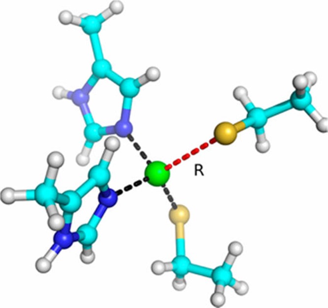
Model system [Zn(Et)₂(Im)₂]⁰ representing the ZnCys₂His₂ binding structure used in fitting the CT and binding energy as a function of the distance between zinc and the ligated atom. Reprinted with permission from ref (481). Copyright 2013 American Chemical Society.

Figure 22.

QM calculated CT (Δq_ct, NPA charge) at the MP2/6-311++g(2df,p) level as a function of the coordinate bond length for ethylthiolate in ZnCys₂His₂, ZnCys₄, and ZnCys₃His₁ systems. Solid lines denote analytical fitted curves of QM results. Reprinted with permission from ref (481). Copyright 2013 American Chemical Society.

Figure 23.

Interaction energies of ethylthiolate (Et) and [Zn(Et)(Im)₂]⁺ as a function of coordinate bond length. E_qm is the binding energy of Et and the [Zn(Et)(Im)₂]⁺ calculated by Gaussian 09 at the MP2/6-311++g(2df,p) level. E_ele is the electrostatic interaction between Et and the [Zn(Et)(Im)₂]⁺. E_vdw is the van der Waals interaction energy between Et and the [Zn(Et)(Im)₂]⁺, and E_ct is “charge-transfer” energy between Et and the [Zn(Et)(Im)₂]⁺ (E_ct = E_qm – E_ele – E_vdw). Reprinted with permission from ref (481). Copyright 2013 American Chemical Society.

3.5.2. Experimental Data (Especially Free-Energy)-Based Parameters

The free energy is a comprehensive thermodynamic property that is a combination of the enthalpy and entropy for a given system. There are two free energies of interest in chemistry: the Helmholtz free energy from a canonical ensemble (abbreviated NVT) and the Gibbs free energy from an isothermal–isobaric ensemble (abbreviated NPT). For most chemistry applications, these two quantities are generally considered as interchangeable. There are various ways to use simulations to estimate the free energy change of a given process: two of the most important first-principles approaches include the FEP⁴⁸³ and TI methods,⁴⁵³ which are widely used to compute absolute and relative free energies in drug design and other application areas. More approximate methods that also estimate free energy changes include the molecular mechanics Poisson–Boltzmann surface area (MM/PBSA),⁴⁸⁴ molecular mechanics generalized Born surface area (MM/GBSA),⁴⁶⁵ and linear response methods.⁴⁶⁵

The FEP method has been reviewed in detail in the past.⁴⁸⁵ Here, we will highlight work of relevance to the study of metal ions using either the FEP or the TI approach. The FEP method was first proposed by Zwanzig in 1954.⁴⁸³ Valleau and Card used MC simulations coupled with the FEP method to investigate the free energy change of Columbic fluids in 1972.⁴⁸⁶ Torrie and Valleau evaluated the configurational Helmholtz free energy change of a LJ fluid system in 1974.⁴⁸⁷ Mezei et al. estimated the HFE and hydration entropy of water using MC simulations combined with the TI method in 1978.⁴⁸⁸ In this effort, good agreement was obtained between the simulated and experimental values. Tembe and McCammon reported the simulation of the relative binding free energy of a protein–ligand system using the thermodynamic cycle and FEP method in 1984, which opened the use of FEP method to drug design optimization applications.⁴⁸⁹ Jorgensen and Ravimohan determined the relative HFE between methanol and ethane using the TIP4P water model in 1985, yielding good agreement with experiment.⁴⁹⁰ Their simulations showed that the hydrogen-bond network is dramatically diminished only after a 25% decrease in the atomic charge of methanol.

Lybrand et al. studied the relative HFE of Cl^– and Br^– using MD simulations and the FEP method.⁴⁹¹ The SPC water model⁴⁹² was used with LJ parameters for Cl^– taken from the GROMOS force field. The LJ parameters of Br^– were determined such that they reproduced the experimental interaction energy difference between Cl(H₂O)⁻ and Br(H₂O)⁻. The estimated relative HFE value was in good agreement with the experimental value (3.15 kcal/mol calculated versus 3.3 kcal/mol experimental). This was followed by calculations on the relative binding free energy between Cl^– and Br^– ions to SC24 (a macrotricyclic receptor) in water using MD-FEP simulations.⁴⁹³ The resultant relative binding free energy was in good agreement with experiment, further demonstrating the validity and usefulness of the FEP method. In a related effort, Mazor et al. studied the relative HFE of Na⁺ and K⁺ and their relative binding free energy to 18-Crown-6 in methanol using the TI method, and the calculated values were in good agreement with experiment (relative HFE, 19.6 kcal/mol calcd versus 17.3 kcal/mol exp; relative binding free energy, −3.5 kcal/mol versus −2.47 kcal/mol).⁴⁹⁴

Jorgensen et al. reported the estimation of the absolute HFEs of methane, water, and Cl^– using the TIP4P water model in 1989.⁴⁹⁵ The final results gave good agreement with experiment (methane, 2.27 ± 0.3 kcal/mol calcd versus 2.005 kcal/mol exp; water, −6.1 ± 0.3 kcal/mol versus −6.3 kcal/mol; Cl^–, −79.3 ± 2 kcal/mol versus −77 kcal/mol), validating that the FEP method could evaluate absolute HFEs of both neutral, polar, and charged species.

In the previous efforts, the ion parameters were generally created for the study itself or were largely unvalidated in terms of their broader performance. In a pioneering work, Åqvist carefully parametrized a series of ions to match their experimental HFE values. He systematically parametrized the 12-6 LJ potential for the alkali and alkaline-earth metal ions using the FEP method to best reproduce experimental HFEs in 1990.⁴⁶² He argued that for simulations with solutions and biomolecules, targeting the absolute HFEs is the most reliable way to parametrize ion potentials other than to reproduce relative solvation energies between ions. Stote and Karplus parametrized the LJ potential for the Zn²⁺ ion with a modified TIP3P water model in 1995.⁴⁹⁶ Initial parameters were derived from an ion–water PES calculated by Clementi et al. and then refined by treating the experimental RDF (the first and second peaks along with the CN value) and HFE as parametrization targets. MC simulation was used to obtain the RDF and CN, while the FEP/MC method was used to obtain the HFE. Good results were obtained in the test simulations of carboxypeptidase A and carbonic anhydrase, where the nonbonded model yielded accuracy comparable to that of the AMBER force field employing the bonded model. Using the Ca²⁺ LJ parameters from Åqvist and Zn²⁺ LJ parameters from Stote and Karplus, Donini and Kollman used the MM/PBSA method to predict the binding affinity of different ligands to a matrix metalloproteinase (MMP).⁴⁹⁷ The correct ranking of the binding affinities of six ligands was obtained from the simulations, while a better ligand was predicted via modifying the best-binding ligand.

Halgren determined the VDW parameters for a series of ions including H₃O⁺, Li⁺, Na⁺, Mg²⁺, Ca²⁺, high-spin Fe²⁺ and Fe³⁺, Cu⁺, Cu²⁺, Zn²⁺, F^–, Cl^–, Br^–, and OH^– in an extension of MMFF94.⁴⁹⁸ Here, the buffered 14-7 VDW potential function was used. The VDW radius was determined on the basis of the polarizabilities (see eq 53, where C_i is a scaling factor). The polarizability of Zn²⁺ was determined on the basis of the XRD structures, while the polarizabilities of the other ions were derived on the basis of energetic and structural properties of mono- and tri-hydrates for monovalent ions, or tri- and hexa-hydrates for highly charged ions.

53

Peng et al. parametrized the alkali metal ions and halide ions using the 9-6 LJ nonbonded model by treating the experimental LC and LE values as targets.⁴⁹⁹ The Waldman–Hagler combining rules were employed in their work. These parameters obeyed the trend of the noble gas atoms—the VDW radii R_min/2 and dispersion coefficient C₆ increase inside the group, and the isoelectronic relationship that R_min/2 and C₆ of the particles, which share the same electronic structure, follow the sequence anion > neutral particle > cation. These parameters showed good agreement with the QM calculated interaction energies of the monohydrates and experimentally determined IOD values (where the SPC water model was employed in the simulations).

Jensen and Jorgenson parametrized the alkali-metal ions, halide ions, and ammonium ions using the 12-6 LJ potential and the TIP4P water model in 2006.⁵⁰⁰ MC simulations and FEP calculations were used to reproduce the experimental IOD and HFE values, respectively. Geometric combining rules were employed in the simulations. The final parameters were also able to reproduce QM calculated interaction energies of monohydrates and the experimental CN values of these ions. This represented the first self-consistent 12-6 LJ parameter set for halide ions that was parametrized for aqueous-phase simulations.

In an extensive and systematic effort, Babu and Lim parametrized the 12-6 LJ potential for 24 divalent metal ions in 2006.⁵⁰¹ The nonbonded interaction was truncated using an atom-based switching function. Lorentz–Berthelot (LB) combining rules and the TIP3P water model were used during these simulations. The FEP method was used to calculate the relative HFEs, and the experimental HFE values were taken from Marcus’ data set.⁵⁰² Final parameters were determined via their ability to reproduce the relative HFE to Cd²⁺. Overall, their parameter set was able to simultaneously reproduce the relative HFEs, the IOD values, and CNs relative to experiment to a good level of accuracy.

Carlsson and Åqvist calculated the absolute hydration entropies of five alkali metal ions in 2009.⁵⁰³ The hydration entropies were evaluated on the basis of the van’t Hoff plots with HFEs calculated under different temperatures. The simulated hydration entropies agreed well with experiment. They found that the entropy change associated with the creation of a neutral VDW sphere in water solution is correlated with the accessible surface area of the ion in question. It was also shown that without temperature-dependent parameters, neither the continuum Born model nor the linear response approximation could simulate the entropy change associated with charging a VDW sphere in aqueous solution.

Won systematically parametrized 12-6 LJ parameters for monovalent, divalent, and trivalent metal ions to reproduce their experimental HFE values in 2012 using the FEP method.⁵⁰⁴ The LB combining rules and the TIP3P water model were employed in the parametrization effort. Meanwhile, during the simulations, the long-range electrostatic interactions were modeled using the solvent boundary potential along with switching functions for the nonbonded interactions (electrostatic and VDW interactions). To address the nonunique parameter problem (discussed below), for a certain ion, the value of ε was derived from the hydration shell radius and thickness, from which the R_min/2 was determined empirically to reproduce the experimental HFE value.

In 2012, Mao and Pappu developed nonbonded parameters for alkali metal and halide ions for hard-sphere and 12-6 LJ models.⁵⁰⁵ The parameters were designed to reproduce the lattice energies and interionic distances of a number of ionic salts. LB combining rules were used in their work, and they used the parameter consistency criteria proposed by Peng et al.⁴⁹⁹ (mentioned above) as constraints for the parametrization process. Because no water model was considered during the parametrization process, their parameters are independent of water model choice. It was shown that generally the final LJ parameters reproduced the lattice structures (correctly predicts the favorability of FCC over BCC structures for 17 out of 20 salts), and the HFEs of ions (with RMSDs of 1.0, 4.1, and 2.4 kcal/mol for TIP3P, SPC/E, and TIP4P_EW water models, respectively, where the simulated HEFs were determined using the HFE hypersurfaces determined by Joung and Cheatham⁵⁰⁶ and the experimental HFEs were from Schmid et al.⁵⁰⁷), showing excellent transferability. They also discussed that the simulated HFE is particularly sensitive to the LJ parameters of small ions.

Darden et al. developed the particle mesh Ewald (PME) method on the basis of the fast Fourier transform in 1993.³⁷³ It offered a substantial speed improvement (proportional to N log N rather than N² for Ewald sums, where N is the number of particles in the system) coupled with good accuracy. MD simulations of proteins and nucleic acids using this algorithm showed improved stability.⁵⁰⁸ This method can also be used to calculate multipole interactions in periodic systems and has been used with polarizable force fields.⁵⁰⁹ In recent years, the PME method has became the standard technique for MD simulations, essentially rendering the earlier parameters sets somewhat obsolete. In what follows, we introduce several representative works of the reparametrization of the nonbonded model of ions specifically for the PME approach.

In light of this, Joung and Cheatham reparametrized the alkali metal and halide ions in conjunction with the PME method.⁵⁰⁶ They systematically reparametrized the 12-6 LJ nonbonded model for alkali metal and halide ions for three widely used water models (TIP3P, SPC/E, and TIP4P_EW) in 2008.⁵⁰⁶ Importantly, they accounted for long-range electrostatic interactions using the particle mesh Ewald (PME) method as opposed to using a cutoff scheme. The values targeted in the parametrization effort were the experimental HFE, LE, and LC values. These parameters were also able to reproduce the interaction energies of monohydrates and the IOD values.

In recent years, Li, Merz, and co-workers systematically developed 12-6 LJ parameters for monovalent to tetravalent ions for use with the PME model (see Figure 24).^390,391,510 They demonstrated that it is difficult to find accurate 12-6 LJ parameters for divalent metal ions even with the PME method.³⁹⁰ Moreover, the error of the 12-6 LJ nonbonded model increases along with the charge of the ion of interest (i.e., from monovalent to tetravalent).^390,391,510 They developed different parameter sets for various metal ions (from monovalent to tetravalent) aimed at reproducing different experimental properties (HFEs, IODs, relative HFEs, CNs).^390,391,510 Many of their conclusions will be covered in sections 3.6 and 3.7.

Figure 24.

Atomic ions that were parametrized for the 12-6 model by Li, Merz, and co-workers.^390,391,510 These ions are shown with a blue background. The monovalent anions, monovalent cations, divalent cations, trivalent cations, and tetravalent cations are shown in light green, yellow, orange, red, and dark red, respectively. The ions that have multiple oxidation states are shown in white, which are Cr²⁺/Cr³⁺, Fe²⁺/Fe³⁺, Cu⁺/Cu²⁺, Ag⁺/Ag²⁺, Ce³⁺/Ce⁴⁺, Sm²⁺/Sm³⁺, Eu²⁺/Eu³⁺, and Tl⁺/Tl³⁺. Besides these atomic ions, the H₃O⁺ and NH₄⁺ ions were also parametrized in their work. Reprinted with permission from the Ph.D. dissertation of Li.⁵¹¹ Copyright 2016 Pengfei Li.

Fitting LJ parameters for metals proceeds differently from that of the ions. Pairwise potentials including 9-6 LJ and 12-6 LJ models yield impressive performance for metals as well. Recently, metal–protein systems and their associated interactions have attracted considerable attention. CVFF/CHARMM-METAL⁵¹² and Gold-protein (GolP)⁵¹³ are two widely used FF models used to simulate this class of systems. The former was parametrized for a number of FCC metals and surfaces (they specifically examined (111) and (100) surfaces), but did not consider polarization explicitly. The later model includes the polarization effect with the Drude rod (DR) model (see section 6.2.2), and it considers interactions with different natures (e.g., chemisorbed, π systems) separately in the parametrization process, but specific for the Au(111) surface. However, none of them included covalent interactions between metal surfaces and adsorbates. We introduce the CVFF/CHARMM-METAL force field below (which is an unpolarized force field and a part of the INTERFACE force field developed by Heinz et al.), while the GolP force field, which is a polarizable force field, is discussed in section 6.2.2.

Heinz et al. parametrized the 12-6 LJ and 9-6 LJ potentials for FCC metals in 2008.⁵¹² They noted that the parametrization strategy based on deriving the LJ parameters on the basis of density and vaporization energies worked well for the nonpolar organic liquids, but it is not suitable for metallic and mineral systems. The former systems usually have a boiling point ±200 K over room temperature, while for the latter ones they have boiling points up to 4000 K. The assumption that vaporization energies can be employed as the fitting target resulted in low-quality LJ parameters, while density and surface tension properties under standard conditions afforded better fitting targets resulting in higher quality LJ models. In the LJ equation, the R_min and ε are related to the density and surface free energy of the lowest energy (111) surface, respectively. In their work, they used both the geometric combining rules (as in OPLS-AA) and the sixth power combining rules (as in COMPASS), and both of them offered good performance. They found the two parameters are only slightly correlated with each other, implying their different physical roles. Both the 12-6 LJ and the 9-6 LJ equations were parametrized; the latter one has ∼1.7% increase in R_min and an ∼18% decrease in ε due to its less repulsive and more attractive characteristics. It was shown that through use of this strategy, it was possible to decrease the deviation from experiment by about 1 order of magnitude when compared to fits based on the density and vaporization energy. Results show that the newly developed parameters give deviations in the densities (0.1%), surface energies of (100) surfaces (3%), metal–water interface energies (10%), and mechanical properties (25%), when compared to experiment.⁵¹² The 12-6 LJ model outperformed the 9-6 LJ model in reproducing mechanical properties. As compared to semiempirical quantum mechanical methods like the EAM and TB approaches, the new parameters showed comparable accuracy and were up to 1 million times faster.⁵¹² The INTERFACE force field model is discussed further in the bonded model section (Section 4) of this Review.

3.6. Transferability, Physical Meaning, and Balance of the Parameters

3.6.1. Condition Changes

The wide range of parameters that have been developed, to date, employ different simulation conditions (e.g., different cutoff values, long-range interaction algorithms, etc.), which limits the transferability of the derived parameters. This was touched on by Marrone and Merz as well as by Åqvist in the early 1990s.^514−516 When cation and anion parameters, developed on the basis of different parametrization schemes, are used in combination, an imbalance between the parameter sets may occur. For example, Auffinger et al. showed that for the simulation of KCl solutions, the K⁺ parameters of Dang and Kollman⁵¹⁷ showed better performance than the AMBER ones adopted from the work of Åqvist.⁵¹⁸ They also suggested that simulating mixed solutions at concentrations >0.25 M was a better measure of parameter quality than examining them at minimal salt conditions. Importantly, these 12-6 LJ parameters may not be compatible with new simulation protocols including those using the PME algorithm. Examples about parameters designed specifically for the PME approach were introduced in an earlier section (section 3.5).

3.6.2. Parameter Uniqueness Problem

Using the 12-6 LJ model for ions can lead to multiple combinations of LJ parameters (such as R_min/2 and ε) that give similar HFE and IOD values,³⁹⁰ leading to what we will call the parameter uniqueness problem. The problem here is which one to chose to obtain a consistent set of parameters. The multiple parameter sets arise because similar A_ij and B_ij terms can be obtained between the ion and water-oxygen atoms: for a certain R_min/2 and ε, there will be a corresponding bigger R_min/2 and smaller ε, or a smaller R_min/2 and bigger ε, which yield similar A_ij and B_ij terms (see eqs 54 and 55). Meanwhile, the number of atom types would increase dramatically in biomolecular systems. When two different ion parameter sets, which give similar A_ij terms between an ion and oxygen in water, are applied to the same biomolecule, they may give quite different A_ij terms between the same atom type on the biomolecule and the metal ion after applying the combining rules. So how to select the final parameter combination is a problem that needs to be addressed.

54

55

There are various ways to solve this problem. (1) The easiest way is fixing the value of R_min/2 or ε. For example, Dang and co-workers parametrized a series of ions by uniformly treating their ε values as 0.1 or 0.2 kcal/mol.^519−524 Jensen and Jorgensen parametrized their cations and anions using two different ε values: a smaller one for cations (e.g., 0.0005 kcal/mol) and a large one for anions (0.71 kcal/mol).⁵⁰⁰ (2) A second approach is to parametrize the R_min/2 or ε value first and then determine its partner empirically. For example, Won determined the ε values first based on the radius of the charged sphere (r in eq 56) and the thickness of the spherical hydration shell (Δr in eq 56), and afterward obtained the R_min/2 value based on the ε value.⁵⁰⁴ (3) A third approach is to parametrize the potential with two or more different target values. This may not work when the two parametrization targets are correlated with each other like HFE and IOD.³⁹⁰ In Joung and Cheatham’s work, they parametrized the potential primarily to reproduce the HFE value and selected the final parameter set that gave the best compromise between the LE and LC.⁵⁰⁶ (4) Finally, the R_min/2 and ε parameters can be optimized simultaneously. For example, Babu and Lim parametrized the R_min/2 and ε parameters over a series of ions based on a reference ion.⁵⁰¹ Li et al. proposed the noble gas curve (NGC, see eq 57) to describe the relationship between the R_min/2 and ε values quantitatively.³⁹⁰ On the basis of this, the two-dimensional problem can be solved as a one-dimensional one (discussed further below).

56

57

3.6.3. Values of the Parameters

3.6.3.1. Magnitude and Range of LJ Parameters

The parameters inside the LJ equation can be assigned a physical meaning. For example, R_min/2 represents the VDW radius of the ion, while ε represents the interaction well depth (or mutual energy). On the basis of their physical meaning, we can estimate the appropriate magnitudes and ranges for atomic particles. R_min/2 should have a magnitude appropriate for an atomic particle with respect to their known physical sizes and should be in the range of 0.8–3.0 Å, while ε should be less than 10 kcal/mol or even smaller than 1 kcal/mol due to the overall weakness of the VDW interaction.

3.6.3.2. Insights from Experiment and Theory

Even though it is hard to obtain the VDW radius of a certain ion from experiment directly, we can use the VDW radii of noble gas atoms, as well as that of the element’s neutral form, to estimate its magnitude and range. Moreover, it is possible to obtain theoretical estimates of the VDW radii of some ions.⁵²⁵ All of these values can help us to estimate, determine, and evaluate the final VDW parameters. Using the noble gas atoms as an example: the experimentally determined VDW radii of He, Ne, Ar, Kr, and Xe are 1.40, 1.54, 1.88, 2.02, and 2.16 Å, respectively,⁵²⁶ while their experimentally determined R_min/2 parameters for the 12-6 LJ equation are 1.485, 1.55, 1.88, 2.00, and 2.20 Å, respectively.⁵²⁷ Even though the two sets are not identical (except for the Ar atom), largely because the 12-6 LJ potential is not entirely physically accurate, they are very close in value to one another (with an unsigned average error of ∼0.02 Å).

3.6.3.3. Behavior within a Group

Noble gas atoms have increasing R_min/2 and ε values inside the group. This is because the bigger atom has a more dispersed and polarizable electron cloud. For instance, the R_min/2 parameters of He, Ne, Ar, Kr, and Xe were summarized above, while the experimental ε parameters are ∼0.02, ∼0.08, ∼0.28, ∼0.40, and ∼0.55 kcal/mol, respectively.⁵²⁷ This trend is also predicted by the Slater–Kirkwood formula³⁷⁷ that shows that the mutual energy is correlated with the polarizability of the particle (see eq 25). In eqs 54 and 55, the A_ij and B_ij terms will also increase along with the R_min/2 and ε values. This trend should also be seen inside the alkali ion, alkali-metal ion, and the halide ion groups; that is, the R_min, ε, A, and B values are expected to increase inside these groups as well.

3.6.3.4. Particles Sharing the Same Electronic Structure

Another boundary condition that can be exploited in ion parametrization is the trend among ions that share the same electronic structure. For instance, F^–, Ne, and Na⁺ share the same electronic structure, but the R_min/2 of F^– should be the biggest because it has the smallest nuclear charge resulting in the largest electron dispersion extent. This means F^– will also have the largest ε, A, and B values as well.

3.6.3.5. From Qualitative to Quantitative Relationships

The previous two relationships can help us estimate or evaluate the final parameters qualitatively but not quantitatively. Because the value of ε increases along with the R_min/2 value, Li et al. proposed the use of the NGC (see Figure 25),³⁹⁰ which is fitted from experimentally determined R_min/2 and ε parameters of the noble gas atoms, to quantify the correlation between R_min/2 and ε. This approach converts the two-dimensional parametrization problem (via scanning R_min/2 and ε at the same time) into a one-dimensional problem (only scan R_min/2, while the ε values are calculated from R_min/2 according to the NGC). Moreover, parameters determined using this technique satisfy the two trends described above. Meanwhile, the final determined R_min/2 values based on the NGC were also very close to theoretically estimated VDW radii, further supporting this overall strategy. In addition, the final parameters evaluated in this manner showed excellent transferability when applied to ion-pair solutions,⁵¹⁰ further demonstrating the strength of this approach.

Figure 25.

Determination of the three parameter sets for the Zn²⁺ ion in TIP3P. Reprinted with permission from ref (390). Copyright 2013 American Chemical Society.

3.7. Limitations of the 12-6 Lennard-Jones Model

The 12-6 LJ nonbonded model remains a fast and practical way to simulate ions using classical force fields. Ramaniah et al. studied K⁺ in aqueous solution using the Car–Parrinello MD method (CPMD) in 1999.⁵²⁸ The BLYP functional was used for the system containing a K⁺ ion and 59 water molecules. In total, 0.168 ps of equilibration and 1.98 ps of sampling were performed in the NVE ensemble. Good agreement between the CPMD and classical MD simulations was obtained for the structural properties of aqueous K⁺, validating in part the classical representation of the K⁺ ion. Moreover, it has also shown that it is possible to simultaneously simulate two or more experimental properties for some of the monovalent ions (e.g., Na⁺, K⁺, Rb⁺, Cs⁺) using the 12-6 LJ nonbonded model.⁵¹⁰ Even so, akin to the situation for unpolarized water models where it remains a challenge to reproduce various experimental properties, it also remains for the classical nonbonded model of ions.

3.7.1. Combining Rule Approximations

There are various combining rules that are employed with the LJ equation. These combining rules are based on empirical relationships or on approximate theoretical derivations.^{446,529−537} For example, the Lorentz combining rules are based on the hard sphere approximation.⁵²⁹ Because ion parameters are usually designed for aqueous phase-single ion systems, it is a challenge to accurately simulate VDW interactions inside mixed systems based on the single particle LJ parameters and combining rules coupled with the two-body potential. For example, the LJ parameters generated directly on the basis of combining rules can yield erratic results when simulating counterions at high concentrations, and this can be solved by refitting the LJ parameters between a cation and anion (which is equivalent to using modified combining rules), or via the charge scaling technique introduced in section 3.9.

Fyta and Netz found that the Kirkwood–Buff integrals of some ion pairs were hard to reproduce simply by using the LB combining rules with ion parameters based on single-ion properties.⁵³⁸ This is because the LB combining rules give a smaller C₁₂ for the smaller alkali metal–halides (e.g., NaF), while a bigger C₁₂ for the larger alkali–halide pairs (e.g., CsCl). They introduced scaling factors into the LB combining rules for the alkali metal-halide LJ parameters, which allowed them to reproduce the Kirkwood–Buff integrals.

Luo and Roux have shown the LJ parameters based on LB combining rules failed to reproduce the osmotic pressure of high concentration solutions, and they successfully refitted the LJ parameters between the cations Na⁺, K⁺, and the anion Cl^– to reproduce osmotic pressure up to solubility limits (see Figure 26).⁵³⁹ Furthermore, the inaccuracy of the combining rules for highly concentrated solutions exists not only for the nonbonded model, but also for other models including the cationic dummy atom model (CDAM) and polarizable models. Related discussions can be found in section 5.1 and section 6.

Figure 26.

Osmotic pressure as a function of the NaCl (a) or KCl (b) salt concentration. The red line is the experimental values; green line is obtained from MD simulations with the LB combination rules; blue line and magenta line are from simulations with adjusted R_min LJ parameters using NBFIX. In panel a, the blue line is the original Na⁺ (1) from ref (540), and the magenta line is the reparametrized Na⁺ (2) from ref (541). The error bars are calculated from 10 separate trajectories of 1 ns. Reprinted with permission from ref (539). Copyright 2010 American Chemical Society.

3.7.2. Influence of the Water Model

Moreover, the water model, which was used to do the original parametrization work, is another factor that influences the overall quality of the ion parameters. Joung and Cheatham performed an investigation on their previously developed parameters (which were obtained by fitting to experimental HFE, LE, and LC values) to reproduce several experimental solution properties such as solubility, activity coefficients, diffusion coefficients, association constants, and residence time of atomic pairs.⁵⁴² They reached the conclusion that the water model has a significant influence on the reliability of the ion force field; therefore, concomitantly developing a reliable water model is very important. They also found that the SPC/E and TIP4P_EW water models were preferred over the TIP3P water model to simulate solutions with high salt concentrations. Moreover, the nature of the ion–ion interaction is crucial to reproduce solution properties such as cation–anion residence time, association constant, solubility, etc.

Note that there are water model-independent ion parameters available including those from Peng et al. (9-6 LJ model)⁴⁹⁹ and Mao and Pappu (hard-sphere model and 12-6 LJ model)⁵⁰⁵ where the parameters were fit for crystalline properties. These parameters could be a choice if the water–ion parameters coupling issue can be ignored in the particular application.

3.7.3. Limitations of the 12-6 Lennard-Jones Potential for Ions

Li et al. observed that it is difficult (and in some cases likely impossible) to find LJ parameters that simultaneously reproduce experimental HFE and IOD values for the divalent and higher-charged metal ions in PME-based simulations.^390,391Figure 27 showed that it is impossible to simultaneously obtain a LJ parameter combination to reproduce both the HFE and the IOD values of these divalent ions. Moreover, with increasing ion radii, the error of the 12-6 model decreases (the HFE and IOD fitting curves are the closest for the biggest ion, Ba²⁺). It is possible to reproduce both properties simultaneously for some monovalent cations (including Na⁺, K⁺, Rb⁺, Cs⁺), while for cations that can strongly polarize the surrounding water molecules (like Li⁺, Ag⁺, Tl⁺) difficulties arise (see Figure 28, left panel). Meanwhile, as shown in the right panel of Figure 28, it is also hard to reproduce both properties simultaneously for halide ions due to the charge hydration asymmetry.⁵¹⁰ Generally, it was found that the error of the 12-6 LJ nonbonded model is approximately proportional to the square charge of the metal ion (see Figure 29).⁵¹⁰

Figure 27.

HFE and IOD fitting curves of six representative divalent metal ions using TIP3P water model. Reprinted with permission from ref (390). Copyright 2013 American Chemical Society.

Figure 28.

Fitting curves between the HFE and IOD values for the positive (left) and negative (right) monovalent ions with three water models together with the targeted values of the ions investigated in the work of Li et al.⁵¹⁰ Reprinted with permission from ref (510). Copyright 2015 American Chemical Society.

Figure 29.

HFE absolute errors (left) and percentage errors (right) for the IOD parameter sets for the mono-, di-, tri-, and tetravalent cations in the TIP3P water model. The ratio is roughly 1.0:3.0:4.8:14.2 for the errors in the HFE values for the mono-, di-, tri-, and tetravalent cations. This agreed well with the ion-induced dipole interaction (eq 59) that predicts that strength of the ion-induced dipole is approximately proportional to the square of the ion’s charge (ratio of 1²:2²:3²:4²). Reprinted with permission from ref (510). Copyright 2015 American Chemical Society.

These drawbacks of the 12-6 LJ nonbonded model leads to fine-tuning or refitting the parameters to meet different demands in a simulation. Generally, because most of the parametrization was performed to reproduce structural (e.g., IOD, LC, etc.), thermodynamic (e.g., HFE, LE, etc.), and microscopic (e.g., monohydrate interaction energy) properties, the parameters underperform in reproducing kinetic (e.g., exchange rate, activation energy) or macroscopic properties (e.g., osmotic pressure). Instead of changing the two parameters in the LJ equation simultaneously, researchers tend to fine-tune one specific parameter (e.g., R_min/2, σ, C₆). Generally, larger adjustments are needed for the highly charged ions, for which the 12-6 LJ nonbonded model yields its most significant errors.

Allnér et al. parametrized the Mg²⁺ ion by adjusting the C₆ value to reproduce the experimental exchange rate of its first solvation shell water molecules.⁵⁴³ They refitted the parameters because previous Mg²⁺ parameters gave Mg²⁺–water exchange rates several orders of magnitude smaller than the experimental value. The potential of mean force (PMF) between the Mg²⁺ and oxygen atom in water was calculated, which was coupled with transition state theory to estimate the exchange rate. Tests were carried out for Mg²⁺ binding to a monophosphate model system and Mg²⁺ binding to the RNA purine riboswitch add A-riboswitch.⁵⁴³ The parameters generated by these authors showed improved performance in the reproduction of kinetic properties.

Yoo and Aksimentiev parametrized the Li⁺, Na⁺, K⁺, and Mg²⁺ ions for nucleic acid systems to reproduce the experimental values for osmotic coefficients.⁵⁴⁴ Available parameters were unable to reproduce the arrangement and inner pressure of a DNA array consists of 64 parallel duplex DNA. Multiple LJ σ parameters involving nonbonded interactions were adjusted (see Figure 30), and the dipoles of the six coordinated water molecules to the Mg²⁺ ion (still represented by the nonbonded model) were enlarged by 1 D to follow the results of the AMOEBA polarizable force field. With these modifications, they were better able to reproduce the experimental osmotic coefficients and DNA array properties. Venable et al. also revised the LJ radii for the Na⁺ ion and other organic groups to reproduce experimental osmotic pressures in sodium acetate and electrophoretic results on vesicles of palmitoyl-oleoylphosphatidylcholine.⁵⁴⁵ Even with only small adjustments (changing the LJ radii by only 0.02–0.12 Å), the new parameter set alleviated the issue of Na⁺-lipid overbinding and increased the surface area by 5–10% per lipid.

Figure 30.

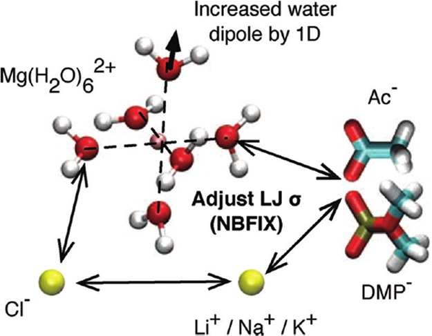
Illustration of the reparametrization scheme used in the work of Yoo and Aksimentiev.⁵⁴⁴ Oxygen is colored in red, magnesium in pink, carbon in cyan, phosphorus in tan, hydrogen in white, and salt ions in yellow. Reprinted with permission from ref (544). Copyright 2012 American Chemical Society.

Torras and Aleman parametrized the Cu⁺, Cu²⁺, and Zn²⁺ ions in acetonitrile using the 12-6 LJ potential in conjunction with Ewald sums to estimate long-range electrostatic interactions.⁵⁴⁶ The parametrization targets were experimental solvation free energies, ion–N distance at the first peak of the RDF, and the CN value of the first solvation shell. The TI method combined with MD simulations was used to obtain the solvation free energy. To reproduce the experimental solvation free energy, the ion–N distance was underestimated about 0.21, 0.28, and 0.12 Å for Cu⁺, Cu²⁺, and Zn²⁺, respectively, when compared to the experimental values. They needed to increase ε to rather large values (63.0, 285.0, and 410.0 kcal/mol for Cu⁺, Zn²⁺, and Cu²⁺, respectively) and keep the R_min/2 values relatively small (0.230, 0.4565, and 0.413 Å for Cu⁺, Zn²⁺, and Cu²⁺ ions, respectively) to reproduce the experimental HFEs.

de Araujo et al. parametrized the 12-6 LJ potential for Cd²⁺ and Pb²⁺ to reproduce the experimental HFE, experimental, and QM/MM calculated RDF and CN values.⁵⁴⁷ The HFE values were evaluated using the linear interaction energy (LIE) method. The parameters were optimized using the TIP3P water model and were subsequently tested in another three water models (SPC, SPC/E, and TIP4P). The calculated HFE values have errors in the range of 57.04–253.21 kJ/mol (∼13.63 to ∼60.52 kcal/mol) when compared to available experimental values. The four-site TIP4P water model had the largest error relative to the other three three-site water models. The results showed that Cd²⁺ has a smaller diffusion coefficient and a longer MRT in its first solvation shell when compared to the Pd²⁺ ion.

Williams et al. created 12-6 LJ parameters for the Fe³⁺-ethylenediamine complex with H₂O, Cl^–, TcO₄^–, and SO₄^2– ions.⁵⁴⁸ The resultant LJ parameters showed limited transferability for the highly charged Fe³⁺ ion. They optimized the LJ parameters for different ligand types via reproduction gas-phase interaction energies from DFT calculations. The final optimized σ values for the Fe³⁺ ion for different ligands were 1.465 Å (for O in H₂O), 1.820 Å (for O in SO₄^2–), 2.600 Å (for O in TcO₄^–), 3.095 Å (for Cl^–), and 1.700 Å (for other atom types), whose variation arises due to different polarization magnitudes between Fe³⁺ and its ligands. PMF profiles generated using the umbrella sampling method were used to estimate the affinities between the complex and its ligands. The calculated results agreed well with the ligand exchange mechanism proposed from experiments. Moreover, they found that both the relative solvation enthalpy and entropy are important for the ligand exchange process.

3.8. 12-6-4 Nonbonded Model

Li and Merz proposed a 12-6-4 LJ-type nonbonded model in 2014.⁵⁴⁹ Overall, they parametrized the 12-6-4 model for various ions from monovalent to tetravalent for three widely used water models (see Figure 31).^391,510,549 It was based on the consideration that classical force fields do not explicitly consider the charge-induced dipole and dipole–induced dipole interactions (see Figure 32), and that the former term is proportional to r^–4 (the latter term is also included in the r^–4 term akin to how the dipole–dipole interaction is present in the point charge model). Hence, a C₄ term was used to represent the ion-induced dipole interaction and was added to the standard 12-6 LJ equation (see eq 58). It was shown that after carefully designing the parameters, both the experimental HFE and IOD values could be simulated at the same time, even for the halides and highly charged ions. Through a consideration of the physical origin of the C₄ term (see eq 59 for the charge-induced dipole interaction energy and eq 60 for the C₄ term), a different combining rule was proposed (see eq 61), and it gave excellent transferability when applied to various systems (such as proteins, ionic solutions, and DNA systems).^391,510,549 For example, in the work of Li et al., the 12-6-4 model showed improvement over all 12-6 models tested in reproducing the KBIs of ionic-pair solutions.⁵¹⁰ Panteva et al. found that the 12-6-4 model was an improvement over 12-6 models in simulating the Mg²⁺ ion in aqueous solution.⁵⁵⁰ They also observed that the 12-6-4 model of Mg²⁺ with the SPC/E water model largely reproduced all relevant experimental properties (such as RDF, HFE, exchange barrier of first solvation shell water, diffusion constant, etc.) simultaneously. This independently validated that the 12-6-4 model, which provides a better physical description than the 12-6 LJ model, was capable of simultaneously reproducing various properties.

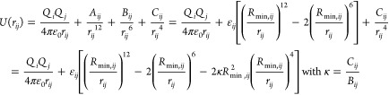58

59

60

61

Figure 31.

Atomic ions that were parametrized for the 12-6-4 model by Li, Merz, and co-workers.^391,510,549 These ions are shown with a blue background. The monovalent anions, monovalent cations, divalent cations, trivalent cations, and tetravalent cations are shown in light green, yellow, orange, red, and dark red, respectively. The ions that have multiple oxidation states are shown in white, which are Cr²⁺/Cr³⁺, Fe²⁺/Fe³⁺, Cu⁺/Cu²⁺, Ce³⁺/Ce⁴⁺, and Tl⁺/Tl³⁺. Besides these atomic ions, the H₃O⁺ and NH₄⁺ ions were also parametrized in their work. Reprinted with permission from the Ph.D. dissertation of Li.⁵¹¹ Copyright 2016 Pengfei Li.

Figure 32.

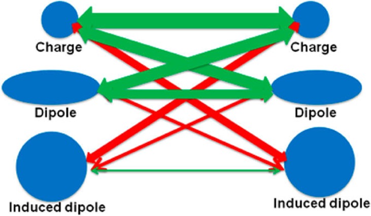
Scheme representing intermolecular interactions: the green double-headed arrow and red double-headed arrow represent the interactions, which are included and not included in the 12-6 nonbonded model, respectively. Reprinted with permission from ref (549). Copyright 2014 American Chemical Society.

In Table 2, we compare the 12-6-4 models to polarizable and the PBE functional for the simulation of aqueous Mg²⁺ system. It was shown that the 12-6-4 models outperform all of the other models listed. This may due to that the 12-6-4 potential better encapsulates the physics associated with Mg²⁺ interacting with water molecules.

Table 2. Comparison of DFT, Polarizable, and 12-6-4 Models for Simulating the Mg²⁺ Ion in the Aqueous System^a.

model	IOD (Å)	CN	exchange rate (s–1)	diffusion coefficient (10–5 cm2/s)	HFE (kcal/mol)
CPMD/PBE551	2.13	6	<3.2 × 1011
SWN4-NDP552	2.06	6		0.82	–447.2
AMOEBA-J553	2.07	6	4.4 × 109	0.3	–431.1 ± 2.9
AMOEBA-P554	2.08	6	<2.0 × 108
FQ-DCT555	2.06	6		0.34 ± 0.4	–461.6
12-6-4 TIP3P	2.09549	6549	5.2 × 107550	0.813 ± 0.059550	–436.6549
12-6-4 SPC/E	2.09549	6549	5.5 × 105550	0.748 ± 0.044550	–436.7549
12-6-4 TIP4PEW	2.09549	6549	1.1 × 107550	0.801 ± 0.052550	–437.9549
experiment	2.09 ± 0.04556	6556	(6.7 ± 0.2) × 105557	0.706558	–437.4502

^aThe two AMOEBA models were differentiated by the first character of the names of the first authors. The exchange rate in the CPMD/PBE simulation is calculated on the basis that water exchange was not observed under 3.1 ps simulation. The exchange rate in the AMOEBA-J simulation is calculated on the basis of the relaxation time of the first solvation shell water molecules as 228 ps. The exchange rate of the AMOEBA-P simulation is calculated on the basis that water exchange was not observed under 5 ns simulation.

Recently, Panteva et al. studied the divalent metal ion–nucleic acid systems employing the 12-6-4 model.⁵⁵⁹ They refit the original 12-6-4 potential to best reproduce binding free energies between different divalent metal ions (Mg²⁺, Mn²⁺, Zn²⁺, and Cd²⁺) with different nucleic acid sites and applied these parameters to the study of metal ion transfer in the hammerhead ribozyme catalytic reaction.

3.9. Charge Scaling Technique

3.9.1. Method Introduction

Unpolarized force fields use simple point charges with VDW spheres that do not afford a good description of short-range and long-range polarization effects (the long-range effect could also be called the charge screening effect). For example, it is hard to reproduce the dielectric constants of organic solvents and water, which results in errors in the description of the long-range interaction between solvated groups. To address this problem, the charge scaling (CS) technique has been developed to simulate long-range screening effects.

Leontyev and Stuchebrukhov created the molecular dynamics electronic continuum (MDEC) method for organic molecules,⁵⁶⁰ water,⁵⁶¹ and ionized groups.⁵⁶² Widely used water models including TIP3P (with a dipole moment of 2.35 D),⁴⁴⁹ SPC/E (2.35 D),⁵⁶³ TIP4P/2005 (2.305 D),⁵⁶⁴ TIP4P_EW (2.32 D),⁵⁶⁵ and TIP5P (2.29 D)⁵⁶⁶ all underestimate the dipole moment of water, when compared to experiment and ab initio MD simulations, which place the dipole moment of water in the liquid phase around ∼3.0 D.⁵⁶¹ Leontyev and Stuchebrukhov explained this by noting that the water dipole moment in the typical unpolarized water models (∼2.3 D) is scaled by a factor of due to the screening effect of the electronic polarization, where ε_el is the high-frequency (electronic) dielectric constant of water, and in their work they used a value from experiment (ε_∞ = 1.78, where ε_∞ is the optical dielectric constant of water) as ε_el for charge scaling.⁵⁶¹ They also proposed that ionized groups (e.g., ionized groups in amino acids, ions) should be scaled down by ∼0.7, while this factor ranges from ∼0.7 to ∼0.9 for neutral groups.⁵⁶⁷ Furthermore, they also developed a fluctuating charge type water model that is compatible with widely used unpolarized force fields such as CHARMM and AMBER, based on the charge scaling concept.⁵⁶⁸ Other than immediately responding to the change of environment, their model represents the water dipole response to environmental changes in a mean-field manner. Even though their model does not simulate the out-of-plane polarizability of water, it does simulate the different extents of the polarization for water molecules coordinated to ions, around protein surfaces, and in the bulk phase. This model can be viewed as a bridge between unpolarized and polarized force fields.

3.9.2. Advantages

The CS technique retains the simulation performance of unpolarized force fields because no additional terms added, while at the same time it better models a number of properties than unscaled unpolarized force fields and even some polarizable force fields (sometimes a reparametrization of the LJ parameters is needed). For example, the CS unpolarized force field reproduces the PMF between one cation and one anion in benzene solution calculated based on the Drude oscillator model.⁵⁶⁷ It also reproduces the dielectric constants of alkanes, which are hard to reproduce by using unscaled unpolarized force fields.⁵⁶⁷ Even scaling down charges will underestimate HFEs of ions; it was noted that by adding up the electronic free energy term, which usually accounts for more than 50% of the total HFE, the experimental HFEs of polyatomic ions can be well reproduced using this model.⁵⁶⁷ Other studies have shown that the CS technique allows unpolarized force fields to better simulate electric conductivity,⁵⁶⁹ dependency of the water diffusion constant on salt concentration,⁵⁷⁰ structures of highly concentrated ionic solutions,⁵⁷¹ and even interfacial affinities at the water/decane interface.⁵⁷² Herein, we use the water diffusion dependency on salt concentration as an example to illustrate the potential of this method.

Researchers have found that it is challenging to reproduce the increase in the water diffusion coefficient along with the concentrations of ionic solutions with salts that have low charge densities (e.g., CsI), while unpolarized force fields and even some polarizable models predict a decreasing trend as the salt concentration increases. Studies have shown that the charge-transfer effect is important in predicting these trends and that the CS technique can be used to solve this issue.

Kim et al. have studied water diffusion in salt solutions using both MD and NMR techniques.⁵⁷³ They found that both unpolarized models (4 total) and polarizable models (the SWM4-DP and AMOEBA models) could not reproduce the increase of the water diffusion constant concomitant with the CsI salt concentration. Ding et al. have shown that ab initio MD simulation (revPBE DFT functional⁵⁷⁴ was used in their work) could qualitatively reproduce the different dependencies of water diffusion constant on the salt concentrations of NaCl and CsI.⁵⁷⁵ They noted that ab initio MD simulation can simulate the dynamic heterogeneity of waters, which is essential in reproducing these trends.

Kann and Skinner have studied ionic solutions using a CS unpolarized model.⁵⁷⁰ They used the factor (where ε_sim and ε_exp are the simulated and experimental static dielectric constants of water) to scale the ions’ charges. This kind of scaling well reproduces ionic interactions in the aqueous phase since . They used the ion parameters from Mao and Pappu⁵⁰⁵ because these parameters were designed to reproduce the lattice energies and interionic distances, and therefore are not dependent on the water model employed. When their scaling model was used with the TIP4P/2005⁵⁶⁴ or E3B⁵⁷⁶ water model, it reproduced the trend of the water diffusion constant in different concentrated CsI solutions qualitatively. Moreover, the CS ion model with the E3B water model reproduced the reduced mass densities, first peaks of the ion-oxygen RDFs, and diffusion coefficients of ions in various salt solutions. Meanwhile, they discussed that the CS technique may not be well suited to more complicated systems with multiple dielectric environments, and they also noted that the CS technique needs further modification to accurately predict thermodynamic properties.

Li and Wang developed unpolarized models for Na⁺, K⁺, Cl^–, and Br^– ions,^577,578 where a different potential function, other than the standard 12-6 LJ nonbonded model, was used. The adaptive force matching method was employed to reproduce MP2 calculated properties. In their model, these ions have charges other than their formal charges: with cations they have a charge of +0.804e, while anions all have a charge of −0.804e, respectively. These parameters reproduced several properties including salt concentration-dependent water diffusion constant trends. Yao et al. have simulated NaCl and KCl solutions using the FQ-DCT model (see section 6.4.2).⁵⁷⁹ It was found the FQ-DCT model, which incorporates charge-transfer effect in its formulation, qualitatively reproduced the slightly increasing trend of the water diffusion constant with the KCl salt concentration. They discussed that explicit consideration of the charge-transfer effect is important to simulate the different dependencies of water diffusion constant with respect to the concentrations of the Na⁺- and K⁺-containing salt solutions.

3.9.3. Limits

Even though encouraging results were obtained using charge scaled unpolarized force fields, this model’s success is limited and likely will not replace polarizable force fields, which consider polarization effects explicitly. This is mainly because that the charge scaled method is based on an average point of view. Even though it yields excellent performance for the prediction of some statistical properties, it fails to represent the microscopic interactions in the local region.

For example, Schroder compared a CS unpolarized force field with the DO polarizable model for ionic liquids by investigating structural and dynamical properties.⁵⁸⁰ He found that the CS unpolarized force field cannot reproduce the broad range of dipolar distributions simulated by the polarizable force field. Furthermore, inconsistencies in the computed RDFs exist within an 8 Å range, but diminish at longer distances. Schroder also noted that the polarization effects of charge–dipole and dipole–dipole have r^–3 and r^–6 dependencies, respectively, while the charge scaled unpolarized force field has a r^–1 dependence. However, at the macroscopic level, he found that the CS method reproduced the frequency-dependent generalized dielectric constant via the application of a scaling factor of (S^eff)⁻² (herein S^eff is the charge scaling factor), and this factor can be explained using the electronic continuum model.

Pegado et al. have simulated NaSO₄ solutions using a CS unpolarized force field and the DO polarizable force field.⁵⁸¹ Experimental and ab initio MD results were used as reference to evaluate the performance of these force field models. They found that the CS model has a comparable solvation structure, while the DO model predicted an overstructured solvation shell, when compared to the ab initio MD results. They also found the CS model underestimated ion association while the DO model overestimated ion association, when compared to experimental results. Vazdar et al. have found that a CS unpolarized model offered consistent results with experiment and polarizable simulations about the interfacial affinities of halide ions at a water/decane interface (water and decane have electronic dielectric constants of 1.78 and 2, respectively), while simulations based on unscaled model yielded incorrect behavior. However, the unpolarized model overestimates the surface affinities of these ions at the water/vapor interface where the electronic dielectric constant jump is too precipitious.⁵⁷²

3.10. Ion Models in Coarse-Grained Force Fields

Coarse-grained (CG) simulation has become popular in recent years to model macromolecules due to its improved computational performance relative to traditional all-atom simulations. The smallest units in CG models are groups/beads rather than atoms. CG force fields generally use similar functional forms (e.g., bond, angle, dihedral, electrostatic, and VDW terms) as all-atom force field models. The united-atom model is an early example of CG force fields, where CH, CH₂, and CH₃ groups were treated as “united” atoms.³⁹² Different CG models have different coarse-graining levels, but to retain a correct physical representation certain criteria should be met during the coarse-graining process.¹⁵¹ The number of particles in the system decreases along with the increase in the coarse-graining level, and CG models can usually employ much larger simulation time-steps (e.g., a 20–40 fs time-step is used with the MARTINI force field,^152,582 as compared to the 1–2 fs time-step usually used in all-atom simulations). All of these savings dramatically increase the simulation time scale of CG models. Furthermore, it is also possible to build a QM/MM/CG multiscale model to increase the speed of QM/MM simulations.⁵⁸³ The nonbonded model of ions is usually employed in CG force fields. Ion modeling in CG force fields usually treats the atomic ion with its first solvation sphere as a united CG particle.^152,582,584 Because atomic ions are independent from other particles while CG and all-atom models use similar functional forms, CG models of ions can be used both in CG models and in cases where all-atom models are used to represent other features of the system of interest.⁵⁸⁵ Moreover, an all-atom ion model can be used with CG representations for other groups.⁵⁸⁶ However, it was noted that because it is still challenging to simulate atomic ions accurately in the all-atom force field model, the CG model affords only qualitative accuracy.⁵⁸²

Singh et al. simulated a DNA fragment using MD simulations with and without hydrated counterions in 1985.⁵⁸⁵ The AMBER ff84 force field³⁹² was used to model DNA, while a 12-6 LJ nonbonded model with R_min/2 = 5.0 Å, ε = 0.1 kcal/mol, and a 131 amu mass was used to model the hydrated Na⁺ ion to mimic the hydration effect and prevent contact ion pair formation with the negatively charged phosphate groups. Results showed that even though the average structures of the two simulations were similar, the simulation with the counterions predicted a better helical structure when compared to experiment.

Marrink et al. developed a CG force field for lipids (a prototype of the MARTINI force field), in which Na⁺ and Cl^– ions were also parametrized.⁵⁸⁴ The hydrated Na⁺ or Cl^– ions were treated as a “Q” type CG bead and further clarified as a “da” subtype group (a group with both options of acting as a hydrogen-bond donor and acceptor). The interaction between the ions and their environments was represented by a 12-6 LJ model in which the Na⁺ and Cl^– ions were treated with the same VDW parameters. Partial charges of the hydrated Na⁺ and Cl^– ions, which were optimized to reproduce the pair distribution functions from all-atom simulations, were determined to be +0.7e and −0.7e, respectively. The authors discussed that these reduced partial charges simulate the charge screening effect of the first solvation shell. Meanwhile, a relative dielectric constant ε_r = 20 was used to calculate the electrostatic interaction in the force field to include explicit screening. Because of the short-range nature of electrostatic interactions in the model, the authors noted that it is limited to modeling ionic solutions with moderate to high concentrations. In the MARTINI force field, Marrink et al. used formal charges for the CG beads of hydrated Na⁺ and Cl^– ions, together with a reduced relative dielectric constant of ε_r = 15 for the electrostatic calculation in their force field.⁵⁸² These two effects counteract each other and yield reasonable agreement with CNs for ion pairs and ion–solvent simulated using an all-atom model.

Khalili et al. created Ca²⁺ parameters for ion–amino acid interactions in the united residue (UNRES) CG force field.⁵⁸⁶ The Ca²⁺ ion was represented independently rather than as a hydrated ion. The functional forms for ASP/GLU-Ca²⁺, ASN/GLN-Ca²⁺, and normal side chain-Ca²⁺ interactions were treated differently on the basis of the natures of their interactions, while the Ca²⁺–Ca²⁺ interaction was described using a 12-6 LJ nonbonded model. The parameters were fitted to the restricted free energy surfaces, which were obtained using RHF/6-31G** calculations and with a consideration of the degrees of freedom lost during the coarse-graining process. Calculations showed the CG model is effective in predicting the positions of Ca²⁺ ions in proteins.

4. Classical Modeling of Metal Ions: The Bonded Model

4.1. Functional Form and Early Metalloprotein Modeling

4.1.1. Functional Form

The modern bonded model (see eq 62) has the following form: it consists of bond, angle, and dihedral terms for the bonded interaction, with addition of the electrostatic (fourth term) and VDW (fifth term) for the nonbonded interactions. The force field contains a number of parameters to be determined: the k_r (bond force constant) and r_eq (equilibrium bond length) for each bond type; k_θ (angle force constant) and θ_eq (equilibrium angle value) for each possible angle type; V_n (torsion barrier), n (periodicity), and γ (phase) for each possible dihedral type; partial charge q for each atom; and VDW parameters A_ij and B_ij for each atom pair type (these parameters can be calculated on the basis of R_min/2 and ε for each atom type through various combining rules, as discussed in the nonbonded model approach section).

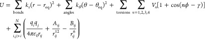62

Lifson and co-workers developed the bonded model for different organic molecules and biomolecules in 1960s and 1970s.^{388,587−595} Their pioneering force field work facilitated the computer modeling of biomacromolecules.⁵⁹⁶ Bixon and Lifson studied the cycloalkanes in 1967.⁵⁸⁷ Besides the bonded interactions, only the nonbonded interaction between hydrogen atoms was modeled with an exp-6 representation, while the rest were set to zero. They noted that the dihedral term was the softest term in the energy function and that the conformational strain energy is the most sensitive to the barrier height of the dihedral angles rather than other force constants.

Lifson and Warshel proposed the “consistent force field” (CFF) for cycloalkanes and n-alkanes in 1968.³⁸⁸ The force field parameters were optimized to best reproduce several experimentally observed values. In this work, they found notable improvements by (1) incorporating the Coulombic term and(2) using a Urey–Bradley function (for 1–3 interactions) and the 12-6 Lennard-Jones equation instead of the exp-6 representation.³⁸⁸ In 1969, Levitt and Lifson followed up this work by performing the energy minimization on myoglobin and lysozyme using a united atom model, in which each heavy atom and its connected hydrogen atom(s) were represented by one united particle.⁵⁹⁷ They used the force field shown in eq 62 without the Coulombic term coupled with a restraint term to prevent the final structure deviating far away from the experimental structure. Minimizations were performed with a steepest descent algorithm, and different restraint values were investigated. However, they noted that the force field parameters used had limited accuracy and needed further improvement. Extension of this force field to other organic/biological molecules including amides, lactam rings, alkanes, olefins, peptides, and proteins was reported in a series of papers from the Lifson laboratory.^588−592 In the CFF parametrization work on peptides and proteins by Hagler et al. in 1974, the authors found that the 12-6 and 9-6 LJ functional forms worked equally well when combined with the Coulombic term. Moreover, they observed that an explicit hydrogen-bond term was not needed in their model.⁵⁹¹ In subsequent work of Lifson et al., they also observed that hydrogen bonds were well described using a model consisting of an electrostatic term and a VDW interaction term.⁵⁹⁵

Unlike the bonded terms that are localized, the nonbonded terms are long-range and affect a model’s ability to accurately reproduce interfacial properties.⁵⁹⁸ Atomic charges play a significant role in determining the quality of a force field.⁵⁹⁸ To reproduce different properties simultaneously, it is essential to assign chemically reasonable atomic charges and VDW parameters. For example, partial charges represent electronic localization in the system, and VDW radii should be consistent with experimental values and their intrinsic trends, while the ε values should be relatively small due to VDW interactions being intrinsically weak.

To date, eq 62 and its variants (e.g., instead of 12-6 LJ using a 9-6 LJ for the VDW interaction) represent the most widely used form for a classical force field (see Figure 33). Heinz and co-workers developed the INTERFACE force field, which uses the harmonic force field format (represented by the bond and angle terms in eq 62), for a series of material systems such as silicates, metals, apatites, cement minerals, clay minerals, etc.⁵⁹⁸ In their work, they discussed that even more sophisticated force fields exist, which usually require more parameters and are less transferable. The harmonic force field form has been parametrized for a wide range of biological and material systems (including AMBER,^392−400 CHARMM,^401−406 OPLS-AA,^407−411 and GROMOS,^599−605 for biologically related systems, while COMPASS,^606,607 CVFF,⁶⁰⁸ PCFF,⁶⁰⁹ and TraPPE⁶¹⁰ are more materials orientated). Their electrostatic terms usually use the same Coulombic form, but their LJ terms vary to some extent. For example, different VDW potentials, combining rules, and 1-4 nonbonded scaling schemes are used among them (see Figure 33).

Figure 33.

Available force fields and challenges in transferability. (a) Parameters for different energy expressions can hardly processed into a uniform force field for both organic and inorganic components. (b) Harmonic force fields like AMBER, CHARMM, OPLS-AA, and PCFF are similar and contain quality parameters for organic compounds. Bonded terms and atomic charges for newly added compounds are derived in similar manners. Moderate differences in the type of LJ potential, combining rules, and the scaling of nonbonding interactions between 1,4-bonded atoms (1,4 nonbonded scaling) can be overcome by adjustments in σ_0,ii and ε_0,ii to reproduce the same bulk and interfacial properties. Reprinted with permission from ref (598). Copyright 2013 American Chemical Society.

4.1.2. Early Work on Metalloprotein Modeling

Karplus, Case, and co-workers pioneered the early classical modeling of metalloproteins focusing on heme proteins.^611−614 Gelin and Karplus performed molecular modeling studies of a hemoglobin in 1977.⁶¹¹ In this work, they performed a structure minimization and then static analysis based on a united atom force field. A proposed reaction path for a oxygen transferring from the heme group to surface of the deoxyhemoglobin α chain subunit was presented. On the basis of theoretical calculations and their comparison to experimental data, it was shown how the ligation of the heme group changes its geometry and then induces subunit structural changes. The results indicated that if the subunit is in the deoxy state rather than oxy state, the ligation-induced tertiary structural changes would require more energy.

Case and Karplus performed MD simulations to investigate the binding processes of CO and O₂ to myoglobin.⁶¹² Results from MD simulations based on a diabatic representation (a ligand moves around a rigid protein) highlighted two binding paths. An adiabatic representation (allowing protein relaxation during the simulation) was employed to calculate the binding energy barriers. The calculated barriers, which were obtained from an analysis of the conformational relaxation, yielded qualitative agreement with experiment. Moreover, differences between myoglobin and hemoglobin were discussed in the work.

Following this work, Case and McCammon performed MD simulations exploring how an O₂ molecule enters and exits the heme pocket inside myoglobin.⁶¹³ The path was between the distal His and Val residues, while the reaction coordinate was chosen as the distance between the ligand and a “dividing plane” defined by three atoms in the protein. Umbrella sampling was used to compute the potential of mean force (PMF) for the process. The PMF profile predicted a 7 kcal/mol barrier for O₂ exiting the heme pocket, while the potential energy profile showed an energy decrease along the reaction path. These results indicated that entropy played a defining role for the kinetic barrier. The reactive trajectories, which started from snapshots at the top of the barrier, showed that only a small proportion of O₂ molecule recrossed the “dividing plane”, suggesting the transition state theory (TST) could be applied to this process.

Subsequently, Kottalam and Case carried out MD simulations to investigate the process of O₂ exiting from the heme pocket of sperm whale myoglobin.⁶¹⁴ Umbrella sampling studies were performed to generate PMF profiles at different temperatures. The rate constants were calculated on the basis of the TST approximation and full MD simulations, respectively. The computed rate constants at room temperature agreed well with the available experimental data. The transmission coefficients computed using the TST approximation were in the range of 0.8–0.9. It is interesting that for lower temperatures (between 180 and 270 K), there are higher activation energies (∼5 kcal/mol) than at room temperature (<1 kcal/mol). The authors proposed that this non-Arrhenius behavior may due to a “mechanism” change at different temperatures: the rate-limiting step at low temperatures is governed by the opening of the heme pocket to affect ligand escape, while at higher temperature this barrier is decreased due to protein dynamics and the rate limiting-step is influenced by the frequency at which the ligand can escape along the correct pathway.

4.2. Bond and Angle Parameters

In classical force fields, the bond and angle terms are represented as being independent from the nonbonded terms (electrostatic and VDW). Hence, bond and angle parameters can be transferred between force fields using similar potential function representations. However, many classical force fields include 1-4 nonbonded interactions fully or to some extent (via scaling), thereby coupling the dihedral term to the electrostatic and VDW terms. This then requires that dihedral terms be refit during the parametrization process (as discussed in the dihedral section—Section 4.3—in detail) to ensure a high-quality force field.

The bond and angle terms are represented with harmonic terms in the AMBER,^392−400 CHARMM (with an additional 1-3 harmonic term),^401−406 OPLS-AA,^407−411 GROMOS,^599−605 CVFF,⁶⁰⁸ and DREIDING⁶¹⁵ force fields. Higher power terms and cross terms were added to more sophisticated force fields including the MM series (MM2,^51,616 MM3,^51,617−621 and MM4^622−627), MMFF94,^{498,628−633} COMPASS,^606,607 and PCFF.⁶⁰⁹ There are a number of ways to obtain parameters: based on experimental information (e.g., vibrational spectra from infrared (IR) or Raman studies), theoretical calculations (e.g., the PES scanning, the Z-matrix, and the Seminario methods), or empirical relationships (e.g., Badger’s rule).

Even though the Morse potential can represent the anharmonicity of bond vibrations and is generally thought of as a more accurate description for bonded interactions, it has been largely supplanted by the harmonic model for several reasons: (1) only two parameters define a harmonic term (the equilibrium distance and the force constant), while a Morse potential needs three (the equilibrium distance, well depth, and the potential width); (2) most simulations work at equilibrium, which is well represented by a harmonic model, while the Morse potential allows for bond disassociation leading to possible departures from equilibrium; (3) if needed, the anharmonicity of bond vibrations can be incorporated using higher order terms from the Taylor expansion (e.g., by adding the third-order and fourth-order terms).

One basic assumption in force field models of macromolecules is that the parameters from a small representative system can be transferred into much larger systems. Experiment supports this hypothesis that certain bond types (e.g., the C–C single bond between two sp³ carbon) have similar bond lengths and strengths in different environments. Because of limitations in computational power, macromolecules are usually built up using fragment groups whose parameters were fitted to QM or experimental results. During the parametrization process, the equilibrium bond distances and angle values are usually taken directly from the QM optimized or experimentally determined structures. This is a reasonable approach, but not entirely accurate as equilibrium bond and angle values obtained in this way represent a compromise between various interactions, and hence, likely deviate from the values for the isolated bonds and angles.

Moreover, in experimental spectra and QM calculations, unlike classical force field models, the bonded and nonbonded interactions are not isolated but are coupled together, causing both the Wilson method (see section 4.2.1), the PES scanning method (see section 4.2.2), the Z-matrix method (see section 4.2.3), and the Seminario method (see section 4.2.4) to all have issues with double counting. Ideally, it is best to fit bond and angle parameters to various experimental and QM calculated data by “freeing” all degrees of freedom (without any restraints or constraints) in the parameter space. However, this is challenging because too many degrees of freedom are present (discussed in detail in section 4.2.5). There are empirical ways (see section 4.2.7) available to efficiently estimate force field parameters, but the parameters may have limited accuracy. In short, compromises between accuracy and effort are made, and researchers need to make a choice about which method to use to achieve the desired accuracy.

4.2.1. Parametrization Based on Experimental Spectra

Urey and Bradley described what came to be known as the Urey–Bradley force field (see eq 63) in 1931,⁶³⁴ in which they used the first two terms of a Taylor expansion to represent the relationship between the configurational energy and the bond as well as 1-3 distances while assigning a harmonic function for the angle term. Vibrational frequencies can be calculated on the basis of the potential, and they found that experimental frequencies were best reproduced via addition of a 1/rⁿ term (with n = 5–9) and an electrostatic term (1/r) into the potential.

63

Wilson proposed a method in 1939, which directly generated the expanded secular equation for the vibrational frequencies of a given molecule.⁶³⁵ As shown in eq 64, the B matrix is a vector matrix that transforms a Cartesian coordinate (x_i) representation to an internal coordinate one (R_k), from which the G matrix is created (see eq 65). On the basis of the assumption that the molecular kinetic energy only consists of harmonic vibrations, and through the construction and solution of the secular equation: |F – Gλ| = 0 (where F is the force constant matrix), force constants could be directly evaluated.

64

65

However, in the spectroscopic force field, the F matrix contains the bond, angle, and torsion terms along the diagonal and the cross interactions in the off-diagonal terms. These terms contain the nonbonded interactions implicitly, reducing the transferability of the parameters to disparate systems.⁵¹

Simanouti explored the use of the Urey–Bradley force field and Wilson’s method for a range of molecular systems.^636−638 For example, in one publication, 102 fundamental frequencies of 16 small molecules (with CX₄, CX₃Y, CX₂Y₂, CXY₃ structures) were well reproduced (1.4% mean deviation relative to experiment) based on 28 force constants.⁶³⁶ He also found that the experimental frequencies of CH₄, CD₄, C₂H₆, C₂D₆, (CH₂)_n, and (CD₂)_n were well reproduced using the same force constant parameter set.⁶³⁶ In a subsequent work, he proposed a force field for a range of carbides and silicides.⁶³⁸

Nakagawa and Shimanouchi detected of a series of aquo complexes of TMs using IR spectra.⁶³⁹ On the basis of their experimental studies, they calculated the bond stretching force constants for various metal–oxygen bonds. The strength of these force constants varied according to the sequence: Cr³⁺ > Ni²⁺ > Mn²⁺ ≈ Fe²⁺> Cu²⁺ ≈ Zn²⁺ > Mg²⁺. Their results showed that the largest force constant (the force constant of the Cr³⁺–O bond) is smaller than the force constants found between metal ions and nitrogen atoms in amine/nitro complexes, and between metal ions and carbon atoms in cyanide complexes.

Moreover, it is possible to calculate the IR/Raman spectra using a force field and to fit the force field parameters to reproduce experimental spectra. For example, in the INTERFACE force field developed by Heinz et al.,⁵⁹⁸ the equilibrium bond lengths and angle values were obtained from crystal structures, while the bond and angle force constants were fitted to reproduce experimental IR/Raman spectra. The calculated spectra were based on the Fourier transform of the velocity autocorrelation function. Deviations of less than 50 cm^–1 in the frequencies were achieved when compared to experiment, while the intensities were poorly reproduced because of the classical representation.

4.2.2. Potential Energy Surface Scanning Method

A straightforward way to obtain force field parameters is fitting the force constants based on QM calculated PESs. To illustrate this approach, we give two examples.

In 2012, Shahrokh et al. developed a force field for different heme states representing the cytochrome P450 catalytic cycle.⁶⁴⁰ The parametrization was performed in an AMBER-compatible manner using the B3LYP/LACVP level of theory for the reference QM calculations. Their approach involves two different models (a truncated one and full description) for each state. The bond and angle force constants were obtained on the basis of the QM PES scans of the truncated model. The restrained electrostatic potential (RESP) charges obtained from the full model showed better performance than those from the truncated model in docking studies. They observed different docking patterns of substrate with different models and states, and the parameters showed stability at the nanosecond time scale under a variety of circumstances (with explicit or implicit solvent, with and without the enzyme environment).

Neves et al. developed bonded models for 12 Mn containing complexes from 9 protein systems in 2013.⁶⁴¹ They used the PES scanning method to determine force constants of the bonds and angles involving the metal ion. Partial charges were derived using the RESP charge fitting algorithm. MD simulations were carried out for these systems, and the resultant trajectories were analyzed. Good agreement between the QM and MM models was obtained on the basis of comparisons of the optimized structures and the calculated normal-mode frequencies. They also performed linear and quadratic fits of the bond force constants and equilibrium distances between the Mn ions and their ligating O and N atoms. These fits provide a basis for an empirically derived force field for Mn containing complexes.

The PES scan approach has as its main merit its overall simplicity, but unlike the Z-matrix or Seminario methods, which can obtain all needed bonded parameters in “one-shot”, the PES scanning method requires an independent PES scan for each bond and angle involving the metal center. This makes this approach computationally more expensive than alternatives. Moreover, double counting is still an issue. Fitting all of the energy changes along a PES scanning into a single bond or angle term is not entirely valid because along the PES scanning not only the bond length or angle magnitude changes, but also the related nonbonded interactions (even they are assumed small). Hence, this approach double counts the nonbonded interactions into the degrees of freedom on fitting. This problem could be solved through considering changes of the nonbonded interactions or by using an alternative strategy such as the automated parametrization method (see section 4.2.5).

4.2.3. Z-Matrix Method

There are a number of ways to calculate the Hessian matrix (see eq 66, where F_ij is an element in Hessian matrix with respect to the coordinates of atoms i and j). For example, one can calculate the numerical derivative of the energy or calculate the analytical derivative of the energy (as with the gradients, most modern implementations of QM methods obtain the second derivatives analytically^642,643).

66

Pulay developed a method to calculate force constants on the basis of HF calculations in 1969.⁶⁴⁴ He proposed a method that calculated the derivative of energy analytically and then the second derivative numerically. He called his approach the “force method” in the original article. After calculating the force analytically, one can transform it from Cartesian coordinates to internal coordinates using the Wilson B matrix. This transformation is nonunique so the force constants obtained are dependent on the choice of internal coordinate. He also noted that without explicit electron correlation, the HF method leads to an ionic dissociation picture of a bond and tends to overestimate the bond force constants.

67

Ten years later, Pulay et al. proposed a set of standardized internal coordinates to calculate force constants.⁶⁴⁵ The internal coordinate systems (with coordinates q_i) are complete and nonredundant, which makes eq 67 unique. Their local internal valence coordinates contain the bonds, angles, dihedrals, and their linear combinations. To facilitate force field function construction, a standardized coordinate system was proposed: (1) preferential treatment of the hydrogen atoms due to their small mass; (2) recommended the use of deformational symmetry coordinates with the corresponding planar ring of D_nh symmetry for ring systems; and (3) use of the Simons–Parr–Finlan expansion for the bond stretching coordinate. The resultant force constant matrix can then be used for efficient geometry optimization and transition state searches.

Because of the lack of correlation, the HF method overestimates vibrational frequencies as well as the force constants. Furthermore, anharmonicity lowers the frequencies, thereby further enlarging the overestimation of the vibrational frequencies.⁶⁴⁶ To ameliorate this problem, a scaling factor of 0.9 for the frequencies⁶⁴⁷ and 0.9² = 0.81 for the force constants⁶⁴⁸ was introduced. However, for strongly correlated systems, including organometallics, this scaling strategy may fail. Presently, for this class of problem, DFT offers a better alternative.

Rauhut and Pulay have determined scaling factors for two popular DFT functionals: BLYP and B3LYP, combined with the 6-31G* basis set.⁶⁴⁶ They developed the scaling factors for two different strategies to reproduce experimental vibrational frequencies. The first one uses a uniform scaling factor, while the second one employs multiple scaling factors for different types of internal coordinates (e.g., different bonds, angles, etc.). The uniform scaling factors were 0.995 and 0.963 for frequencies based on the BLYP/6-31G* and B3LYP/6-31G* levels of theory, respectively (for comparison, the HF/6-31G* and MP2/6-31G* scale factors were 0.89⁶⁴⁷ and ∼0.95⁶⁴⁹). Through the use of the multiple scale factor strategy, the B3LYP/6-31G* level of theory gave better performance than the BLYP/6-31G* level of theory.

One drawback of the Z-matrix method is its dependence on the chosen internal coordinates.⁶⁵⁰ For instance, for the three-membered HCON molecule, HF/STO-3G calculations give different force constants for the same CO bond under different internal coordinate choices: the force constant equals (1) 0.54 au when the internal coordinates (excluding hydrogen atoms) are CO, CN, and NCO; (2) 0.57 au when CO, NO, and CON are chosen; and (3) 0.26 au when the redundant internal coordinates CO, NO, CN, CNO, NOC, and OCN are used.⁶⁵⁰ Moreover, in the bonded model, only harmonic terms (which are the diagonal terms in the Z-matrix) are considered, and neglect of the cross terms causes an incomplete description of the potential energy surface (even if some of the cross terms are small). Therefore, force constants obtained using the Z-matrix method may need further adjustments to reproduce QM calculated results (e.g., vibrational frequencies and relative energies). Moreover, the dihedral force constants obtained using the Z-matrix are for the harmonic potential, which are inapplicable to the Fourier expansion series used in contemporary bonded models. This is not only because of the different functional forms, but also because in the dihedral interactions of many force fields, the 1-4 nonbonded interaction is considered either fully or partially, making the dihedral terms obtained from Z-matrix method and force field models incompatible.

Ryde has used the Z-matrix method in his modeling studies of alcohol dehydrogenase, a zinc-containing enzyme, in 1995.⁶⁴⁸ He used the Z-matrix method to obtain the force constants on the basis of HF calculations and then scaled these values by a factor of 0.81 (square of the frequency correction factor). Charges were assigned on the basis of Mulliken charges obtained at the HF level with appropriate adjustments. Minimization results showed that four-coordination was preferred over five-coordination by at least 36 kJ/mol (∼8.6 kcal/mol). He also noted that to correctly simulate the dynamics of the metal site, it is important to use specific force constants for bond stretching, while the application of bond length constraints restricts the sampling space yielding unphysical results.

Tuccinardi et al. studied MMPs, which have a zinc ion in its catalytic site, using a classical force field.⁶⁵¹ The RESP algorithm was used to obtain the partial charges. They obtained the metal–ligand bond force constants on the basis of the Z-matrix method, and represented the angle force constant by scaling down relevant bond force constant by an order of magnitude. These parameters were further optimized to reproduce QM calculated relative energies between different conformations.

Merz and co-workers have studied several metalloproteins based on the Z-matrix method.^652−654 For example, Op’t Holt and Merz performed classical modeling on the human antioxidant protein HAH1.⁶⁵⁴ The Cu⁺ binding site of HAH1 as well as the proposed transfer mechanism for the Cu⁺ ion between the HAH1 and MNK4 proteins are shown in Figures 34 and 35, respectively. However, the original calculated force constants were too weak to reproduce the geometry of the binding site, and were increased to closely reproduce the Cu⁺–S distance in the complex. A larger VDW radius parameter for the Cu⁺ ion was used to prevent close contact between the metal ion and H/S atoms in nearby Cys residues, which are not bound to the metal ion. MD simulations were carried out, and they generally reproduced the XRD structure for the protein and its metal site. Both the QM and the MM results suggested that the Cu⁺ ion prefers two-coordination or three-coordination over four-coordination.

Figure 34.

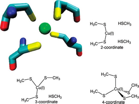
Cu⁺ binding site from the HAH1 crystal structure, including Cys side chains, and the three QM models used to represent two-, three-, and four-coordinate Cu⁺ environments. Reprinted with permission from ref (654). Copyright 2007 American Chemical Society.

Figure 35.

Proposed mechanism for transfer of Cu⁺ between HAH1 and MNK4. A possible four-coordinate intermediate that would reside between the two three-coordinate states in the middle has been left out. In the HAH1 homodimer used as a mimic of the HAH1-MNK4 heterodimer in MD simulations, C14 and C17 of the target domain are replaced by Cys 12 B and Cys 15 B, respectively. Reprinted with permission from ref (654). Copyright 2007 American Chemical Society.

4.2.4. Seminario Method

The Seminario method and its associated software, FUERZA, were described in 1996.⁶⁵⁰ This method reproduced the vibrational frequencies of several small molecules (including a Rh complex) as demonstrated by Seminario.⁶⁵⁰ It uses a sub matrix of the Cartesian Hessian matrix to calculate force constants. It reduces the 3N × 3N matrix problem into a problem involving 3N 3 × 3 matrixes. The parametrization process is straightforward and does not involve an iterative process. The parameters derived on the basis of the Seminario method employ a harmonic approximation for the bond, angle, dihedral, and improper torsion terms (see eq 68). The geometric parameters r_eq, θ_eq, ϕ_eq, and ω_eq can be obtained on the basis of QM optimized or XRD structures, and the force constant parameters k_b, k_θ, k_ϕ, and k_ω are derived on the basis of eqs 69–72. In these equations, k_AB is the force constant between atom A and B, while u_AB is the unit vector between the two atoms. λ_i and v_i are the eigenvalues and eigenvectors of the sub Hessian matrix between atoms A and B. In total, there are three eigenvectors of each sub Hessian matrix. u^N is the unit vector perpendicular to the BCD plane. u^PA and u^PB are the unit vectors perpendicular to unit vector u^AB and u^CB; R_AB and R_CB are the bond distances between atoms AB and CB; u_NABC and u_NBCD are the unit vectors perpendicular to planes ABC and BCD, respectively.

68

69

70

71

72

Note that the Seminario method incorporates the influence of the environment implicitly in its parametrization. The force constants can be considered as “effective force constants” and may not be accurate for isolated bonds, angles, dihedrals, and improper torsion terms. Moreover, the dihedral and improper torsion parameters obtained from the Seminario method are not directly applicable to force fields such as AMBER, CHARMM, OPLS-AA, GROMOS, etc., due to differences in functional forms (herein harmonic terms are used while these force fields all use a Fourier expansion). Furthermore, explicit 1-4 nonbonded interactions in these force fields create further complications. In related applications, only the bond and angle parameters based on the Seminario method are used, while the dihedral and improper torsion terms involving metal ions are set to zero.^1,655−660

The Seminario method showed its versatility in applications to various systems. For example, Seminario and co-workers derived force field parameters for oligopeptides,⁶⁶¹ polypeptides,⁶⁶² nitro compounds,⁶⁶³ Si nanoclusters,⁶⁶⁴ and gallium nitride nanoclusters⁶⁶⁵ on the basis of the Seminario method. Some other applications including ionic liquids,⁶⁶⁶ carbon nanotubes,⁶⁶⁷ and MOFs⁶⁶⁸ were also reported. Below we highlight some examples about metal-containing systems.

Nilsson et al. developed the program, Hess2FF, on the basis of the Seminario method in 2003.⁶⁶⁹ They pointed out that the sub matrix could be selected in two different ways for each atom pair, the (i,j) or (j,i) submatrix, and found it led to less than 5% uncertainty in determining the force constants. They averaged the final result on the basis of various possible permutations. They refined five heterocompounds in protein systems (three containing one iron or zinc ion) by utilizing the Hess2FF software. They calculated the Cartesian Hessian matrix using the B3LYP functional, AM1, and PM3 SE-QM methods, as well as the universal force field (UFF), DREIDING, and MMFF94 force fields. They found that the B3LYP functional performed best according to the R_free factor, and it was recommended for high accuracy calculations. On the basis of force field parameters obtained from B3LYP calculations using mixed basis sets (6-31G* basis set for main group atoms and a double-ζ with polarization basis set for the TMs), they performed XRD structure refinement using the Crystallography and NMR System (CNS) force field, and obtained high-resolution structures with decreasing R_free factors. In particular, a 1.70 Å resolution structure of cytochrome c₅₅₃ matched a 0.97 Å resolution structure more closely after the refinement with parameters obtained by Hess2FF. In the refinement process, they used the harmonic approximation for the dihedral term and did not include electrostatic term. However, they proposed that the electrostatic term should not be neglected for polar systems in classical simulation.

Lin and Wang parametrized 18 zinc-containing complexes, in which the metal associated bond and angle parameters were obtained from the Seminario method and charge parameters were derived using the RESP algorithm based on the B3LYP/6-311++G(2d,2p) level of theory.⁶⁵⁵ The metal related torsion parameters were set to zero, while the remaining force field parameters were obtained from GAFF. They tested their models with different combinations of the bonded/nonbonded model with RESP charge/formal charge schemes. Ultimately, they found that the bonded model using a RESP charge model performed the best among all strategies examined. They performed normal-mode analysis for four different systems, and good agreement was obtained between MM and QM calculated results. Some inconsistencies existed for the high frequency modes, and they showed that the agreement could be improved by tuning bond parameters involving hydrogen. They also noted that these modifications were not necessary when the SHAKE algorithm was used to constrain X–H bonds during MD simulations.

Peters et al. developed the metal center parameter builder (MCPB) within the modeling toolkit plus plus (MTK++) package to facilitate the building of metal centers in metalloprotein systems.¹ To balance the accuracy and computational cost, a side chain model was created to obtain metal–ligand related bond and angle parameters based on the Seminario method, while a large model (with metal site residues capped by ACE and NME residues) was built to derive partial charges for the metal center based on the RESP algorithm. Furthermore, four charge fitting algorithms (ChgModA, where all of the charges are flexible in the metal cluster; ChgModB, where the charges of the heavy backbone atoms in the metal cluster are fixed; ChgModC, where the charges of all backbone atoms in the metal cluster are fixed; ChgModD, where the charges of all backbone atoms and the C_β atom in the metal cluster are fixed) were tested, and it was found that the ChgModB performed the best when combined with the Seminario method. This may be due to the fact that the charges of the backbone heavy atoms were taken into account in the parametrization of the backbone torsion parameters. On the basis of the Semnario/ChgModB method, they developed the zinc AMBER force field (ZAFF) for 10 different zinc sites with tetrahedral coordination.

Subsequently, there were a number of parametrizations of metalloprotein systems described in the literature based on MCPB. For example, Merz and co-workers studied the Zn-containing protein CzrA,⁶⁵⁶ the Cu-containing metallochaperone CusF(657) and CusB,⁶⁵⁸ and the Ni-containing enzymes, urease⁶⁵⁹ and Helicobacter pylori (Hp) urease,⁶⁶⁰ based on the MCPB software package using the Seminario method and RESP algorithm. MD simulations were performed, and insights into the structure, function, and dynamics of these metalloproteins were obtained. Below we highlight several of these studies.

In one example of their work, Klebsella aerogenes (KA) urease was studied,⁶⁵⁹ which is a homotrimer of heterotrimers (in total there are nine monomers; see Figure 36), with each homotrimer having an active site that contains a dinickel metal center (see Figure 37). MD simulation of KA urease predicted a “wide-open” state for the flap over the active site (see Figure 38), which was not observed in the available crystal structures. Results showed that the “wide-open” state could be accessed from the “open” state through a relatively low free energy barrier (see Figure 39). This results in a more extensive active site region, which offers further opportunities for structure-based drug design.

Figure 36.

Initial structure of K. aerogenes urease in the open state, as used in the simulations of ref (659). The trimeric subunits are shown in yellow, pink, and cyan. The flaps are shown as α-helices (blue) and loops (red). Nickel ions are shown as green spheres. Reprinted with permission from ref (659). Copyright 2012 American Chemical Society.

Figure 37.

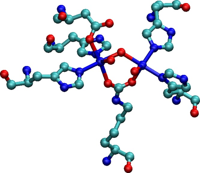
Heavy atoms of the metal site residues in native KA urease. The two nickel ions in the metal center are six-coordinated (left one) and five-coordinated (right one), respectively. The structure is from PDB entry 1FWJ, and this figure was made using VMD.⁶⁷⁰

Figure 38.

Flap, active site, and ancillary binding pocket of K. aerogenes urease. The flap is shown in yellow, the active site in red, and the ancillary binding pocket in blue. The nickel ions are shown as green spheres, and the exposed nickel surfaces in (D)–(I) are also shown in green. The three rows from top to bottom show the closed flap (A–C), the open flap (D–F), and the wide-open flap (G–I). In each row, three views are shown: from the top, looking down into the binding pockets (A, D, G); from the side (B, E, H); and from the side in a cutaway view (C, F, I). To show the scale, a urea molecule (4 Å across) is depicted at the bottom of the figure. Reprinted with permission from ref (659). Copyright 2012 American Chemical Society.

Figure 39.

Relative free energy map for opening of the urease flap. The points labeled as “C”, “O”, and “W”, respectively, represent the closed, open, and wide-open structures shown in Figure 38. Points C and O represent the initial XRD structures of the closed- and open-flap models (PDB entries 1FWJ and 1EJX, respectively); for the latter structure, the flap was added by homology modeling. Point W is a representative wide-open conformation selected from the simulation trajectory of 1FWJ. Reprinted with permission from ref (659). Copyright 2012 American Chemical Society.

In another example, the homodimeric Zn²⁺/Co²⁺-responsive transcriptional repressor from Staphylococcus aureus (so-called CzrA) was studied using MD simulations.⁶⁵⁶CzrA has several allosteric states as shown in Figure 40. Each of its two metal binding sites has 3 HIS residues and 1 ASP residue coordinating to the metal center (see Figure 41). The MD simulation of the DNA bound CzrA system captured the switching between its closed to open state due to Zn²⁺ binding. Analysis suggested Zn²⁺ binding quenches the conformational sampling of the CzrA system through a hydrogen-bonding pathway or network, which is in agreement with experimental results. The root-mean-square fluctuations (RMSFs) of different residues for apo-CzrA and its Zn bound form are shown in Figure 42. From this figure, it is clearly seen that the α2, α3+αR, and β1+β2 domains have significantly decreased RMSF values after Zn binding.

Figure 40.

Four allosteric forms of CzrA examined in the study of Chakravorty et al.,⁶⁵⁶ and the associated thermodynamic parameters of the CzrA mechanism. The protein, CzrA, is shown in red, Zn²⁺ ions are in green, and the DNA molecules are blue. These cartoon depictions are snapshots from their MD simulations of these allosteric forms. A negative cooperative allosteric effect of ∼6 kcal/mol is observed on Zn²⁺ binding to CzrA. Reprinted with permission from ref (656). Copyright 2012 American Chemical Society.

Figure 41.

Snapshot of the CzrA metal binding site from the initial structure. The zinc ion is represented as a silver sphere. The metal binding residues include Asp84, His86, His97′, and His100′. These residues also represent the QM region of the QM/MM MD calculations in the study of Chakravorty et al.⁶⁵⁶ Reprinted with permission from ref (656). Copyright 2012 American Chemical Society.

Figure 42.

Plot of RMSF values for the lowest mode of the protein from simulation of Apo·CzrA starting from the apo-crystal structure, and simulation of allosteric switching for Zn·CzrA starting from the 2KJB NMR structure of apo-CzrA in a closed conformation. Reprinted with permission from ref (656). Copyright 2012 American Chemical Society.

Li and Merz recently developed the MCPB.py program within the python metal site modeling toolbox (pyMSMT) software package.⁶⁷¹ It offers a simple and clear workflow for the parametrization process, and supports many more metal-containing systems than did the earlier MCPB program. It supports more than 80 metals with various oxidation states (see Figure 43) and a number of AMBER force fields. Moreover, it supports multiple coordination modes, as well as organometallic systems. Two examples (one for a metalloprotein and the other for an organometallic system) were described on the basis of the Seminario/ChgModB method. MD simulation of the metalloprotein and a normal-mode analysis of an organometallic compound yielded satisfactory results.

Figure 43.

Metal ions currently supported by the MCPB.py program. The metals with a blue background use the VDW parameters from Li et al.,^390,391,510 whereas the metals with a green background use the VDW parameters adapted from UFF. Reprinted with permission from ref (671). Copyright 2016 American Chemical Society.

Recently, Zheng et al. introduced the visual force field derivation toolkit (VFFDT) to derive bond and angle parameters on the basis of the Seminario method.⁶⁷² It can perform parametrization based on the Hessian matrix obtained from several QM packages: Gaussian 03/09,^673,674 GAMESS-US,⁶⁷⁵ Q-Chem,³⁴⁸ ORCA³⁴⁷ (version 3.0), and MOPAC⁶⁷⁶ (version 2009/2012). The visualization interface is an attractive characteristic, and it serves as a complementary tool to the antechamber, MCPB, and MCPB.py programs in the AmberTools software package.

4.2.5. Automated Parametrization Method

Even though force field parameter derivation based on the Hessian matrix is quite straightforward and the results are encouraging, there remains a double counting issue with this approach. This is because the information contained within the Hessian matrix is balanced between the bonded and nonbonded interactions present in the system of interest, causing the nonbonded interactions to be double counted (implicitly considered in the bonded terms while explicitly considered in the nonbonded terms) in the force field modeling.⁶⁷⁷ However, this problem can be overcome by using, what we term, the automated parametrization method (APM). There is no assumption that the equilibrium geometric parameters are the same as the experimental or QM calculated geometries. Moreover, the final comparison is usually made between the same properties from experiment (or QM calculations) and MM calculated ones.

Basically, if the parameter space dimension is low, one can scan the parameter space. However, if the dimensionality is high, it is really hard to simply scan because the parameter combinations increase exponentially. One can use a coarse grid at the initial stages of the scan and then a finer one when the optimal parameter region is identified. Yet this still does not effectively deal with high dimension parameter spaces. There are different ways to decrease the parameter space dimensions, for example, dividing the parameter set into several subsets and fitting them sequentially with the other subsets fixed, then iterate until converged results are obtained. It is also possible to decrease the parametrization effort using physical/chemical criteria to shrink the parameter space to scan. For example, in the development of the optimal point charge (OPC) water model, the authors used the lowest order multipole moments of water as a filter for parameter selection.⁶⁷⁸

One widely used method to handle high dimension parameter spaces is to perform parameter optimization akin to geometry optimization. The difference is that parameter optimization minimizes the merit function (e.g., the least-squares difference between the simulated and reference properties) with respect to the parameters, while geometry optimization minimizes the total energy with respect to the Cartesian or internal coordinates. Moreover, in parameter fitting, the derivatives usually need to be calculated numerically. Like optimizing the geometry, it is hard to find the global minima in the variable space during the parameter optimization procedure. Presently, parameter optimization processes typically need “tricks” and human intervention.

To solve the large dimension problem, there are several points that need attention. (1) A good merit function needs to be used. Similar to solving linear simultaneous equations, for which the number of equations should be comparable or more than the number of unknown values, a large quantity of reference data is need to ensure that the parameters are not overfit. Furthermore, different kinds of properties are needed to balance the optimization to decrease the “biases” in parameter fitting. Meanwhile, different modifications can be made to the merit function to obtain fits. For example, different weights can be applied to increase the priority of the properties near equilibrium because of their higher occurrences. Moreover, constraints and/or restraints can be applied to keep the parameters in a physically reasonable range. (2) An efficient optimization algorithm/procedure needs to be used. Various algorithms can be used to minimize merit function: for example, steepest descent, conjugated gradient, simplex, genetic algorithms, the Newton–Raphson method, etc. Each algorithm has its own set of pros and cons. The answer to the question of which algorithm to choose is problem dependent. (3) Similar to geometry optimization, a good initial guess is important as well. If a bad initial guess is made, the parametrization can be easily trapped in poor or “high-energy” local minima. These suggestions are not only for the bonded model parameter optimization, but can also be applied to parameterization of other the bonded model using APM.

Several freely available APM-based programs have been described including Paramfit⁶⁷⁹ and ForceBalance.⁶⁸⁰ Interested readers should consult the literature for further details. Below we introduce several examples of the APM.

In the early development of the CFF model, Lifson and co-workers optimized the force field parameters to best reproduce various observables based on a least-squares refinement. For example, in the initial work on CFF for cycloalkanes and n-alkanes, Lifson and Warshel attempted to optimize the force field parameters to best reproduce the experimental excess enthalpy, equilibrium coordinates, and normal-mode frequencies (with different weighting factors for these data).³⁸⁸ Parameters were determined after convergence was reached in the least-squares refinement.

Norrby and Liljefors developed a generalized automatic parametrization procedure for force fields in 1998.⁵⁰ The illustrative example shown was ethane using the MM3* force field (which uses form similar to the MM3 force field). The reference data contain experimental/QM calculated structural data (bond lengths, bond angles, and dihedral angles) and relative energies, as well as a mass-weighted Hessian matrix based on QM calculation. They discussed that the Cartesian root-mean-square deviation (RMSD) may not be a good metric for evaluating the force field quality, and hence bond, angle, and dihedral values were treated as the fitting targets. They also discussed that the B3LYP/6-31G* level of theory offered the best price/performance ratio for obtaining QM source data. The final target is to minimize the merit function χ² (a least-squares function, see eq 73), while different weights were applied to different properties (100 Å^–1, 2 deg^–1, 1 deg^–1, 100 kJ^–1 mol, and 0.01 kJ^–1 mol Ų amu^–1 for the bond, angle, dihedral, relative energy, and mass-weighted Hessian matrix, respectively). They recommended using a strategy by which optimization was done using a modified simplex algorithm followed by optimization using the Newton–Raphson algorithm with Lagrange multipliers.

73

Rydberg and co-workers developed a transition-state force field for cytochrome P450 systems using the method developed by Norrby and Liljefors (see above).⁶⁸¹ Parameters were trained on the basis of calculated transition state structures and Hessian matrixes of 14 substrate models using the B3LYP functional. Another 10 substrate models were used as a test set. Partial charges were determined using the RESP algorithm, while GAFF was used for the substrates. The transition-state force field (or Q2MM method) was not able to calculate the absolute activation energy, but it could evaluate relative barriers, and predict selectivity. The final parameters showed excellent performance for both the training and the test sets: with RMSDs of 0.01 Å and 1.2° for bonds and angles, and has a 0.99 correlation coefficient between the MM- and QM-derived Hessian matrix elements. The transition state structures for aliphatic hydrogen abstraction were well reproduced, but the DFT calculated energies based on them are still ∼24 kJ/mol (∼5.7 kcal/mol) higher than using the DFT optimized ones. This error decreased to 9 kJ/mol (∼2.2 kcal/mol) when a parameter optimization strategy was also applied to the substrate (instead of using GAFF), further demonstrating the deficiency of the MM optimized structures. The authors proposed that this is due to the simplicity of the bonded model approach.

Hu and Ryde compared different MM models for simulating biologically related zinc complexes in 2011.⁶⁷⁷ They suggested using a nonbonded model with restraints or a bonded model based on the Seminario method for structural metal sites, while the method of Norrby and Liljefors affords a better model for catalytic metal sites. However, while the later method afforded a better model, it is more labor intensive than the former methods after QM calculations. Furthermore, the APM requires significant human intervention. For instance, chemical intuition is needed to check whether unphysical local minima were obtained during the parametrization process.⁵⁰ It was found that for the bonded model to perform optimally, new atom types should be assigned to all of the atoms in the metal site. Moreover, attention should be paid to ensure the hydrogen atoms in negatively charged ligands have been assigned appropriate partial charges (i.e., not negative values).

4.2.6. Burger Method and Partial Hessian Fitting Method

4.2.6.1. Burger Method

Burger et al. proposed a new parametrization method and developed related software (so-called parafreq) in 2012.⁶⁸² It solves each internal coordinate separately instead of solving the full Hessian in internal coordinates. It can determine each bond and angle parameter on the basis of the differences between QM and MM calculated Hessian matrixes and the Wilson B matrix. Dihedral terms were determined via fitting to relaxed QM PES scans. Results showed that this method better reproduced QM-derived frequencies than the GAFF, Seminario, and Z-matrix methods.

4.2.6.2. Partial Hessian Fitting Method

Recently, Wang et al. developed the partial Hessian fitting (PHF) method to fit the bond, angle, dihedral, and improper torsion parameters in the bonded model.⁶⁸³ In this method, they aimed at reproducing the partial Hessian matrix between two particles that are in the bond, angle, dihedral, or improper torsion interaction. Nonbonded interactions with RESP charges and the 12-6 LJ potential were determined in the first stage. Afterward, the dihedral force constants were determined to minimize the least-squares difference between QM and MM calculated partial Hessian matrixes between the two terminal particles (which are 1-4 to each other). The angle, improper torsion (if desired), and bond force constants then were derived sequentially to minimize the least-squares difference of QM and MM calculated partial Hessian matrixes between each of the two terminal atoms. QM optimized bond lengths and angle values were used for the initial equilibrium bond and angle values. To prevent distortion caused by too strong of a 1-4 interaction, a scheme called “Katachi” was used to optimize equilibrium bond and angle values to make the MM optimized structure reproduce the QM optimized bond and angle values within 0.0001 Å and 0.002°, respectively. Twenty-three compounds including three secondary building blocks of MOFs were tested. It was shown that the PHF-K method (with the “Katachi” scheme) outperformed the Seminario-K method and GAFF. The PHF method “decouples” the bond, angle, dihedral, improper torsion, and nonbonded parameters, and can be extended to classical force fields that do not use quadratic representations. In comparison, the Seminario method suffers from the double counting problem and is restricted to the harmonic potential form. Meanwhile, the authors also noted that neither the PHF nor the Seminario method can reproduce the QM calculated low-frequency normal modes.

4.2.7. Empirical Approaches

Intuitively, we expect that the larger is the electronic overlap between two atoms, the stronger is the bond, which results in a larger force constant. For instance, in GAFF,³⁹⁷ the equilibrium bond distances between two sp, sp2, aromatic, and sp3 carbons are 1.1983, 1.3343, 1.3984, and 1.5375 Å, respectively, while the corresponding force constants are 923.7, 569.4, 461.1, and 300.9 kcal/mol·Å^–2, respectively.

A number of authors have developed different empirical rules to estimate the relationship between bond length and the corresponding force constant. A range of different dependencies of the force constant to the bond length were explored, including linear,^641,663 quadratic,⁶⁴¹ cubic,⁶⁸⁴ and even up to the sixth power.⁴⁹⁸

Using the harmonic spring model, the following relationship is obtained, where ω_ec represents the vibrational frequency.

74

Mecke proposed that a relationship exists between ω_e and r_e values for various states of a molecule in 1925.⁶⁸⁵ In 1929, Morse proposed a formula (see eq 75), which is generally valid except for a few exceptions.⁶⁸⁶

75

In 1934, Badger proposed (now known as Badger’s rule, see eq 76) a model for diatomic molecules that described the relationship between a bond length and its associated force constant.⁶⁸⁴ In eq 76, the r_e and k₀ are the bond length and bond force constant, respectively, and d_ij is a constant that is only relevant to the locations of the two atoms (row i and row j) in the periodic table. This formula can be applied to both ground and excited states (although exceptions exist). Moreover, it was shown this rule could also be extended to polyatomic molecules in that internuclear distances could be obtained based on vibrational frequencies.⁶⁸⁷

76

There are empirical methods used to determine the bond and angle parameters in classical force fields. For example, to extend MMFF94,⁴⁹⁸ missing bond parameters can be obtained using eqs 77 and 78. According to eq 77, the bond length can be estimated using the covalent radii of atoms i and j, the difference of the Pauling electronegativities χ_i and χ_j, and a so-called “shrinkage” factor δ. C is a proportionality constant, which was set to 0.050 if either i or j is a hydrogen atom, and 0.085 otherwise, while n is an exponent that was assigned a value of 1.4. The shrinkage factor, which is employed because the MMFF94 force field optimized bond lengths are generally larger than the reference values (from MP2/6-31G* optimized geometries), was set to 0.008 Å. Meanwhile, eq 78, which is an inverse sixth power modification of the Badger’s rule, was utilized to determine the bond force constant.

77

78

79

80

For the angle parameters, an approach proposed by Halgren (see eqs 79 and 80) was used.^688,689 In these equations, Z_i, C_j, and Z_k are parameters related only to the atomic number, D is a factor to represent relative dissimilarity between two bond lengths, and β is a scale factor, which is assigned a value of 1.75 (in the general situation), 85% × 1.75 (if i, j, and k are all in a four-member ring), or 5% × 1.75 (if i, j, and k form a three-member ring).

In GAFF, different empirical equations from MMFF94 are used to derive bond and angle parameters.^397,690 Wang et al. employ eqs 81 and 82 to derive the missing bond parameters, where r_ij and K_r are the equilibrium bond length and bond force constant, respectively. K_ij is an empirical parameter for elements i and j, while m is an empirically derived power parameter. m and ln(K_ij) were determined on the basis of least-squares fitting of ln(K_r) versus ln(r_ij) using data from the AMBER force field. It was observed that optimal m values were 5, 4, and 4 for C–C, C–N, and C–O bonds, respectively. Ultimately, an average value of 4.5 was chosen for m to perform the force constant fitting procedure.

81

82

83

84

Equations 83 and 84 were used to derive missing angle force constants. Herein, Z_i, C_j, and Z_k are the empirical parameters for the first, second, and third atoms i, j, and k in an angle. r_ij^eq and r_jk are the equilibrium distances of the bonds ij and jk, while θ_ijk^eq is the equilibrium value of angle ijk. In the AMBER force field, it was shown for situations where (1) both i and k are hydrogen atoms, (2) only one of the two is a hydrogen atom, and (3) in the remaining situations, the force constant is about 30–35, 50, and 70 kcal/mol·rad^–2, respectively.

In the work of Bellido and Seminario on nitro compounds, which used the Seminario parametrization scheme, a linear relationship was found between the bond force constants and bond distances for bonds without hydrogen atoms (see eq 85 and panel A of Figure 44).⁶⁶³ However, there were no clear trends observed between the angle values and the angle force constants except the C–C–C angle in octanitrocubane (see panel B of Figure 44).

85

Figure 44.

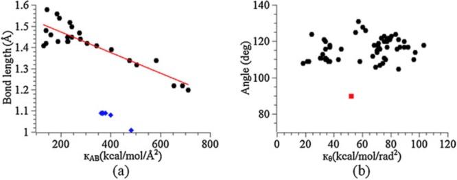
(a) Bond length versus bond force constant; blue ◆ are bonds with hydrogen atoms. (b) Angle versus angular force constant; the red ■ represents the angle between carbon atoms in octanitrocubane. Adapted with permission from ref (663). Copyright 2011 Springer.

Moreover, in the work of Agulira-Segura and Seminario, they found that in general the force constant decreases with the increasing of equilibrium distance for the Si–Si bond.⁶⁶⁴

In the work of Neves et al., the bond and angle force constants were obtained on the basis of the PES scanning method (see section 4.2.2).⁶⁴¹ They performed linear fitting between the bond force constants and the bond distances for the Mn ions and their ligating atoms in different residues. The results are shown in Figure 45. The R² values of these fits are 0.82, 0.86, 0.90, and 0.91, respectively. They also performed quadratic fits between the Mn ions with ligating oxygen and nitrogen atoms (see Figure 46). The R² values of these two fits were 0.92 and 0.91, respectively. Similar to Bellido and Seminario, Neves et al. did not find a clear relationship between the equilibrium angle values and the angle force constants (see Figure 47). However, even with the use of different methods (Seminario versus PES scanning), the results were consistent in showing that the angle force constants were usually under 100 kcal/mol·rad^–2.

Figure 45.

Linear regression for the main ligands in Mn-coordination spheres: aspartate, glutamate, histidine, and water, shown in red, orange, blue, and green, respectively. Reprinted with permission from ref (641). Copyright 2013 American Chemical Society.

Figure 46.

Second-order polynomial regression for the main donor atoms in Mn-coordination spheres (oxygen and nitrogen are shown in red and blue colors, respectively). Reprinted with permission from ref (641). Copyright 2013 American Chemical Society.

Figure 47.

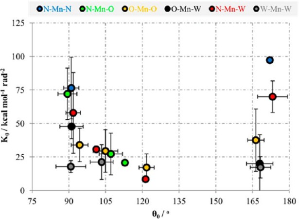
Average equilibrium angles and force constants for main donor atoms concerning the equilibrium angles for the main geometries in manganese. Reprinted with permission from ref (641). Copyright 2013 American Chemical Society.

4.3. Dihedral and Improper Torsion Parameters

4.3.1. Dihedral and Improper Torsion Parameters in Alkane Chains and Protein Systems

The physical meaning of dihedral interactions is the repulsion between electrons clouds in chemical bonds rather than in atoms.⁶⁹¹ It is essential to have the dihedral term to represent the flexibility of the bond rotations within an organic molecule. Overall, dihedral rotation barriers are small for typical organic molecules. For example, there is only a ∼3 kcal/mol (∼5 × RT at T = 300 K) energy difference between the staggered and eclipsed conformations of ethane. Thus, even the high energy eclipsed conformation is accessible at room temperature. In their early force field work on n-alkanes, Bixon and Lifson described the dihedral term as the softest term in the potential function, but makes a significant contribution to the strain energy.⁵⁸⁷

86

Fourier expansion is widely used to represent dihedral interactions. Different terms in the Fourier expansion were used to represent the influence of different structural features (see the first term in eq 86). In some force field models, 1-4 nonbonded terms (see the second term in eq 86, where f_ele and f_VDW are the scaling factors for the 1-4 electrostatic and 1-4 VDW interactions, respectively) are also included to represent eclipsing interactions. Briefly, assigning a periodicity of 1 represents the cis–trans preference (the phase is 0° if trans is more stable than cis, and is 180° for the reverse) where there is only one maximum and one minimum. Assigning a periodicity of 2 yields two maxima and two minima, which represents the rotation in an ethene (with a phase of 180°) and also an out-of-plane improper torsion term (with a phase of 180°). A periodicity value of 3 represents three maxima and three minima, which represents, for example, the rotation of an ethane that has two sp³ hybrid carbons (with a phase of 0°). In reality, multiple terms in the Fourier expansion may be needed to obtain an accurate representation of a specific dihedral, which have, for example, a specific trans–cis preference, different hybridizations of the central two atoms (e.g., sp² and sp³), etc. Moreover, the Fourier equation has also been used to represent the angle bending interaction and offers better performance than the harmonic potential (e.g., in the SHAPES force field,¹⁹⁷ see section 7.1.2).

The 1-4 nonbonded interactions are considered explicitly or implicitly in classical force fields. Hence, the dihedral terms are usually lumped together with the 1-4 nonbonded interactions (containing the 1-4 electrostatic and 1-4 VDW interactions) to facilitate the accurate reproduction of the total bond rotation barrier. There are different scaling factors used for the 1-4 nonbonded interactions. For example, the scaling factor of 1-4 electrostatic interactions (f_ele in eq 86) in the AMBER force field (FF94) was set to 1/1.2, which was fitted from the 1,2-enthanediol molecule and while also showing transferability to other small molecules like amines, butane, and alcohols.⁶⁹² The scaling factor of the 1-4 VDW interaction (f_VDW in eq 86) was set to 1/2 in the FF94 AMBER force field.³⁹⁴ However, the scaling of 1-4 electrostatic and 1-4 VDW integrations is all assigned a value of 1 in the GLYCAM force field.⁶⁹³ In the CHARMM force field (CHARMM 19 force field),^694,695 the 1-4 scaling factors for both the electrostatic and the VDW interactions are 0.4, while in its current version (CHARMM 22/27),^{401,402,696,697} the 1-4 interactions were evaluated without scaling (or with a scaling factor of 1). Clearly, attention should be paid when transferring dihedral parameters between different force fields.

The torsion parameters play an important role in the reproduction of secondary structures and the energy balance between different relevant configurations in biomacromolecules. For example, dihedral parameters relevant to the protein backbone atoms such as C–N–C_α–C, N–Cα–C–N, C_β–C_α–N–C, and C_β–C_α–C–N play, one can say, an outsized role in the simulation of the protein folding processes. Several related force fields have been developed on the basis of QM calculated results, including the AMBER ff03,³⁹⁶ AMBER ff99SB,³⁹⁸ AMBER ff02.pol.r1,⁶⁹⁸ CHARMM CMAP,⁴⁰³ and AMBER ff14SB.⁴⁰⁰

4.3.2. Dihedral and Improper Torsion Parameters in Metal-Containing Complexes

Comba et al. suggested that if metal is in not in the central bond of a dihedral, the dihedral parameters could be treated the same as other dihedrals with the same central bond. If the metal ion is in the central bond of a dihedral, the dihedral parameters are usually assumed to be negligable.¹⁴⁶ Overall, the dihedral and improper torsion terms involving metal ions are usually treated as having a zero barrier height when using classical potentials. For example, in the early work of Hancock, the torsion parameters were typically omitted.⁶⁹¹ In the extensive work of Lin and Wang,⁶⁵⁵ and Peters et al.,¹ modeling Zn complexes in protein system, and the work of Rui et al.⁶⁴¹ modeling Mn-containing protein complexes, setting the torsion terms to zero had no adverse effects. Moreover, in a range of work on metalloproteins from Merz and co-workers,^{652−654,656−660} torsion terms involving metal ions were also treated as having zero barrier heights. In the INTERFACE force field for different material systems, there is generally no dihedral or improper torsion parameter assigned. Furthermore, adding dihedral parameters may cause a problem in MM modeling including metal ions.⁶⁹⁹ Neglecting these terms can be ascribed to various factors including rigidity of the overall complex, high periodicity of TM-based torsion motions, functional form issues, 1-4 nonbonded interaction coupling, small barrier heights, etc., but probably the latter is most often invoked.

4.3.2.1. Rigidity

Bonds become harder to rotate when molecular structures become more “compact”. The bond in a diatomic molecule (e.g., F₂) can be viewed as rotating freely, while for the ethane molecule, which has two connected sp³ carbon atoms with each having 3 bound hydrogen atoms, a rotation barrier (∼3 kcal/mol) is introduced.⁵⁸⁷ TMs usually have large CNs, yielding compact structures, even more so when the ligands are large, and the metal sites in protein systems are even more rigid due to restrictions introduced by the protein matrix. In these situations, large-scale bond rotations are not expected to occur, making the neglection of torsion terms involving metal ions largely inconsequential.

4.3.2.2. High Periodicity and Small Amplitudes

The torsion parameters are usually not considered in TM complexes because of their high periodicity and the notion that the barrier heights are generally low.¹³⁹ Because of the high periodicity of TM complexes, higher Fourier terms may be needed to accurately model the torsion PES. An octahedrally coordinated metal ion has 4-fold rotation barriers; hence a Fourier term with periodicity of 4 will be needed to accurately model this torsion motion. Importantly, more terms in the Fourier function directly result in more complicated parametrization efforts.

Moreover, the torsion barriers for TM complexes are usually small. For example, it was shown experimentally that there is a high frequency rotation of the Cr–N bond in the Cr(NH₃)₆³⁺ system, even at temperatures as low as 20 K.⁷⁰⁰ In the review of Brubaker and Johnson in 1984, the barriers of dihedral and improper torsion potentials are generally small.¹³⁹ Weaver et al. investigated the performance of CCSD and CCSD(T) methods for predicting the HOFs of Zn-containing systems in 2009.²⁰⁵ In this work, they carried out a PES scan of the H–C–Zn–C–H twisted dihedral angle (note this is a 1-5 interaction, see Figure 48) for the Zn(CH₃)₂ complex using the CCSD/6-31G** level of theory. The computed barrier is very small (less than 0.03 kcal/mol, see Figure 49) and is just ∼1% of the barrier observed for the H–C–C–H dihedral angle of ethane (∼3 kcal/mol).

Figure 48.

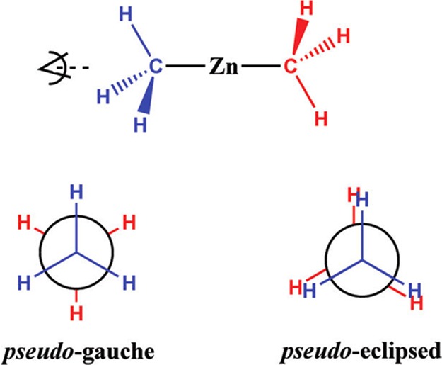
Newman projections depicting viable Zn(CH₃)₂ conformations. Reprinted with permission from ref (205). Copyright 2009 American Chemical Society.

Figure 49.

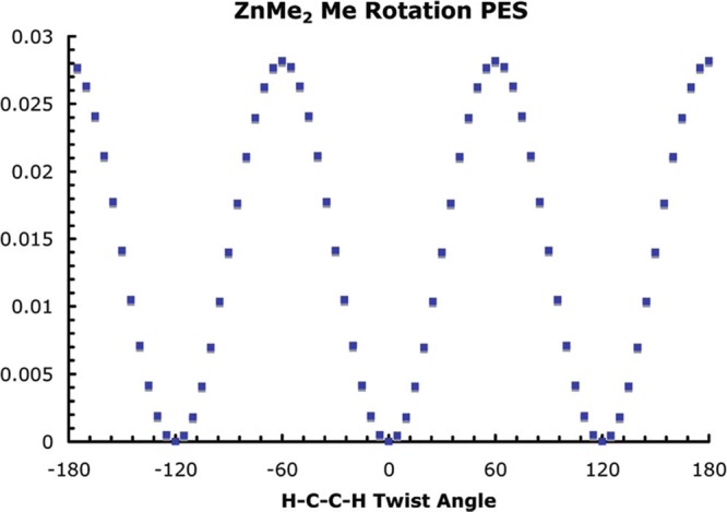
Relative conformational energy versus H–C–C–H twist for ¹Zn(CH₃)₂ (CCSD/6-31G**); unrelaxed scan in 5° increments. Minima at −120°, 0°, and 120° correspond to the pseudoeclipsed conformation; maxima at −60°, 60°, and 180° correspond to pseudogauche. Reprinted with permission from ref (205). Copyright 2009 American Chemical Society.

4.3.2.3. Different Functional Forms

Another reason torsion terms are neglected is that the torsion parameters obtained using “one-shot” methods (such as the Z-matrix and Seminario methods) are for the harmonic equation and cannot be readily applied to Fourier terms directly. For example, Nilsson et al. parametrized the harmonic dihedral parameters (using the CNS force field) for several heterocompounds using the Seminario method and then applied them to XRD refinement with excellent performance.⁶⁶⁹ However, this option is not readily available to fit complex Fourier expansions, making the development of this class of Fourier potentials an even greater challenge.

4.3.2.4. 1-4 Interactions

Moreover, dihedral parameters usually need to be fit under the total or partial consideration of 1-4 nonbonded interactions, making the parametrization process even more complex and time-consuming. Because the scaling factor may vary among different force fields, care should be taken when transferring these parameters for relevant dihedral terms.

4.3.2.5. Examples Obtaining the Torsion Parameters for Metal-Containing Complexes

Burger et al. parametrized the dihedral terms for the dizinc complex of bis-dipicolylamine based on a relaxed PES scan.⁶⁸² Scans along the dihedral with QM and MM (with dihedral terms set to zero for the latter) methods were performed, while the difference was used to fit the Fourier expansion through a least-squares algorithm. A cutoff value of 0.1 kcal/mol for the V_i term (V_i/2 is the rotation barrier) was used to truncate the Fourier expansion. Some other details of their work can be found elsewhere in the present text (section 4.2.6).

In some studies of metal-containing complexes, dihedral or improper torsion terms were included to constrain the planarity of the complex. For example, Hambley investigated the ligand rotation barriers of several Pt complexes (diammine- and bis(amine)bis(purine)-Pt²⁺ complexes) using a classical mechanics force field,⁷⁰¹ in which an improper torsion parameter with a 602 kJ/mol (∼144 kcal/mol) barrier was added to retain the planarity of the Pt complexes. The calculated ligand rotation barriers agreed well with experimental results. Finally, it was shown that the rotation barriers are predominantly influenced by the interaction between the ammine/amine ligands and the 6-position group of the coordinated purine ligands. This research relates to cisplatin and its congeners, while related discussion of the impact of their work on broadening the understanding of this drug class is included in their work.

4.4. Charge Parameters

Similar to force field development for organic molecules, electrostatic terms were usually not considered in early modeling studies of TM complexes.^139,691 Later, as was also concluded for the modeling of macromolecular systems including proteins, the partial charge term is necessary for the accurate representation of long-range electrostatic interactions.⁷⁰²

There are a number of approaches to determine charge parameters: empirical methods, methods based on QM fitting, experimental derivation, FQ method, etc. Empirical charges were mainly used in the early stages of modern force field development, which can be fitted to reproduce experimental structures, energetics, and dipole moments.^591,592,595 CFF^591,592,595 and OPLS^703,704 are two well-known force fields that used empirical charges. However, empirically derived charges offered challenges when trying to represent transition and excited states, while QM calculations could readily generate the needed parameters. Moreover, it is time-consuming to fit empirical charges because of the need of extensive testing using minimization, MC, or MD simulations to reproduce requisite experimental properties. Given these considerations, QM-derived charges tend to be the preferred approach in the design of modern force field models. An intriguing approach involves obtaining charges based on experimental data, and they have been shown to yield excellent performance in classical modeling studies.⁵⁹⁸ Finally, the FQ model is also widely used in contemporary molecular simulation studies, but we defer discussion of this method until section 6.1.

4.4.1. Quantum Mechanics-Derived Charges

There are a number of ways to obtain QM-derived partial charges, all with their associated pros and cons. For example, charges can be obtained using molecular orbital (MO) analysis (e.g., Mulliken,^705−708 NPA,⁷⁰⁹ AOIM⁷¹⁰), based on ESP fitting (e.g., Singh–Kollman,⁷¹¹ CHELP,⁷¹² CHELPG⁷¹³), based on the electron density in real space (e.g., AIM,⁷¹⁴ Hirshfeld,⁷¹⁵ ADCH⁷¹⁶), and then a number of ways to derive charges using postprocessing or scaling techniques (e.g., AM1-BCC,^717,718 CM1,⁷¹⁹ CM2,⁷²⁰ CM3,⁷²¹ CM4,⁷²² CM5,⁷²³). The Mulliken charge, which is based on the Mulliken population analysis, is widely used because it is easy to obtain and has a well-understood physical meaning. However, raw Mulliken charges are not suitable for modeling atomic partial charges directly for use in force field methods. This is because the Mulliken charge is basis set sensitive and does not accurately reproduce the multipolar properties of molecules. Scaling procedures can be effectively applied to Mulliken charges for subsequent use in MM modeling. For example, AM1-BCC charges were based on Mulliken population analysis and then scaled to reproduce HF/6-31G* calculated RESP charges. The CM1 charge model was derived from Mulliken charges and then fitted to experimental properties. Mulliken charges are also used in the SCC-DFTB method (see Section 2.4.4) for the description of changes in the charge.

Partial charges, based on ESP fitting, can accurately reproduce the multipolar properties of molecules and could reproduce intermolecular or intramolecular electrostatic interactions, leading to the conclusion that they provide an excellent choice for partial charges in MM calculations.⁷¹¹

4.4.1.1. Electrostatic Potential Map

Bonaccorsi and co-workers developed the idea of using electrostatic potential maps (EPMs) to study molecular properties in the early 1970s.^724−730 They applied the method to various small molecule systems including diatomic and triatomic molecules,⁷²⁶ three-membered ring molecules,^724,725,728 and nucleic acid bases,⁷³⁰ and the results were insightful in further our understanding of protonation properties or identifying electrophilic sites. Kollman et al.⁷³¹ and Morokuma et al.^732,733 used the EPM method to explore hydrogen-bond interactions and found them to be helpful in predicting the directionality and strength of hydrogen bonds. Kollman and co-workers carried out pioneering studies using QM-derived ESPs maps to explore Coulombic interactions in biological systems. Hayes and Kollman employed ESP maps to investigate protein–ligand interactions between carboxypeptidase A (CPA) and the Gly-Tyr substrate in 1976.⁷³⁴ They predicted that an o-OH-Gly-Tyr analogue would have a stronger binding interaction to CPA than Gly-Tyr.⁷³⁴ In another work, they also explored important electrostatic contributions in the binding pocket that might facilitate catalysis.⁷³⁵ Later, Nuss and Kollman used ESP maps to study the interactions between different base pairs.⁷³⁶ The predicted interactions correlated well with relative biological activities but not as well with relative binding affinities.⁷³⁶

After the application of the EPM method to explore chemical phenomenon, partial charges derived by fitting were determined to reproduce the EPMs and to mimic the charge distribution in a molecule. For example, Bonaccorsi et al. utilized 13 charge points in a single water molecule to represent the QM calculated charge distribution of a water molecule.⁷²⁷ These partial charges were placed on the nuclear centers and the centroids of localized orbitals. These partial charges reproduced the QM-derived EPM reasonably accurately. Afterward, Almlöf and Wahlgren fit the atomic charges of the H₃O⁺ ion via a least-squares fit of the QM calculated potentials on points surrounding the hydronium ion.⁷³⁷

4.4.1.2. QM-Derived ESP Charges

The ESP of a point r in space can be calculated using QM methods based on eq 87, where Z_A is the nuclear charge, R_A is the position of the nuclei, while r′ is a dummy integration variable. i and j are atomic orbital indices, while P_ij is the density matrix. The classical ESP of the same point (at r) is represented by eq 88, where R_A is also the nuclear coordinate. q_A is the atomic charge, for which we want to finally fit, based on a linear least-squares fitting between the V_QM(r) and V_MM(r) values.⁷³⁸ The total net charge is applied as a restraint during the fitting process, while other restraints (e.g., dipole moment, etc.) may also be applied when so desired. The location of the ESP points depends on the algorithm being employed, and different weights can be applied to select ESP points during the fitting process (e.g., making the points that are closer to the nuclei have larger weights).⁷³⁸

87

88

Scrocco and Tomasi,⁷³⁹ Momany,⁷³⁸ Cox and Williams,⁷⁴⁰ and Smit et al.⁷⁴¹ all carried out pioneering works on the determination of atomic partial charges of small molecules based on the EPM. The critical issue was to locate the position and necessary density of points to obtain the best fit of atomic charges to the EPM. It was proposed that the points should not be too close to the nuclei, where the ESP is usually positive.⁷⁴⁰ It was also shown that the root-mean-square (RMS) error of the fit increased when using points close to the nuclei in the fitting process.^711,740 Furthermore, it was found that it was not necessary to considered points that were too far away from the nuclei. Overall, it was found that picking points between the VDW surface and up to 3 or 7 Å away from this surface gave satisfactory results. A total net charge restraint was needed for the ESP fitting procedure, and further constraints could be added for the dipole moment or higher multipole moments as needed. Meanwhile, different weights could be applied to points in different areas of the EPM. For example, Momany used smaller weights on points closer to the VDW surface during the fitting procedure.⁷³⁸ Generally, there are two different ways to choose ESP points: cube-based or layer/shell-based. There is not a clear sense of which approach is the best, and it depends somewhat on the properties to be reproduced.⁷⁴² Momany selected points between the VDW surface and several angstroms away from it, and used a density of 0.5 Å between each point.⁷³⁸ Cox and Williams used a boundary that was 1.2 Å away from the VDW surface, with a shell thickness as 1.0 Å and cubic grid spacing of 1.0–1.2 Å.⁷⁴⁰ Singh and Kollman picked points on a shell around the molecule at 1.4, 1.6, 1.8, and 2.0 times the VDW radius with a density of 1–5 points per unit area.⁷¹¹ The CHarges from Electrostatic Potentials (CHELP) method selected points symmetrically placed on spherical shells around the atomic nuclei with 14 points on each shell. In total, there were 4 shells selected with the innermost as the VDW surface of the molecule and the other shells placed at 1, 2, and 3 Å away from the VDW surface, respectively.⁷¹² The CHarges from ELectrostatic Potentials using a Grid-based (CHELPG) method selects points between the VDW surface of the molecule and a surface 2.8 Å away using a cubic grid with a spacing of 0.3 Å between points.⁷¹³

Singh and Kollman described an algorithm for charge derivation based on fitting point charges to ab initio-derived ESPs and applied it to a selection of small molecules in 1984.⁷¹¹ The Singh–Kollman approach has also been used in the charge determination for united atom models and lone pair sites.⁷¹¹ On the basis of united atom fits, the ff84 AMBER force field was developed for proteins and nucleic acids.³⁹² Chirlian and Francl created the CHELP algorithm and related software to fit atomic charges based on QM calculated ESPs in 1987.⁷¹² They found that the results based on calculations using the HF method with different basis sets (including STO-3G, 3-21G, and 6-31G*) could accurately reproduce QM-derived dipole moments. Finally, they selected the HF/3-21G level of theory as the best method to use based on its speed and overall accuracy. Breneman and Wiberg noted that the CHELP algorithm was inadequate to describe the charge invariance of internal rotations and developed the CHELPG method to alleviate this issue.⁷¹³ Besler et al. carried out a study of ESP charge fitting on a series of organic molecules using the MNDO, AM1, HF/STO-3G, and HF/6-31G* levels of theory in 1990.⁷⁴³ In this work, they found that the MNDO method showed better performance than AM1 and HF/STO-3G calculations when compared to the HF/6-31G* results. Moreover, HF/6-31G* quality ESP charges could be obtained by scaling the MNDO results, which afforded a quick way to derive reliable atomic charges for a classical force field.

Merz and co-workers incorporated the ESP approach in their investigations of human carbonic anhydrase II (HCAII, a zinc-containing enzyme) in the early 1990s.^702,744,745 In their modeling of the metal-containing active site, they used equilibrium bond distance and angle values from QM optimizations based on the MNDO method, the bond and angle force constants from experiment, while the LJ parameters for the zinc ion were obtained such that they reproduced the QM calculated geometries and interaction energies of the Zn²⁺–CO₂ and Zn²⁺–H₂O complexes. It was shown that the metal site experiences a strong electron transfer effect from the coordinating groups to the zinc ion. For example, the MNDO ESP calculations of the [(imidazole)₃Zn–OH]⁺ complex showed a charge of +0.5 on zinc, which is much smaller than its formal oxidation state +2.⁷⁴⁴

By combining the MD and FEP methods, Merz calculated the binding energies of the CO₂ molecule to two different binding sites in the HCAII system.⁷⁴⁴ The results showed good agreement with the experimental values and suggested that the first binding site of CO₂ is catalytically important, while the second binding site, which is further away from the metal site, served to increase the surface area for CO₂ to be recognized and bound by HCAII. In related work, Merz and co-workers performed FEP calculation on several sulfonamide inhibitors bound to HCAII.⁷⁴⁵ Experimental relative binding affinities were reproduced via a consideration of the pK_a differences between the sulfonamide and sulfonate groups. They concluded that a single hydrogen interaction, which is present in the sulfonamides but not sulfonates, was responsible for the higher binding affinity of the former.

Hoops et al. carried out an investigation of different charge modeling strategies on a zinc center coordinated by the side chain nitrogen atoms of three HIS residues and one hydroxide oxygen.⁷⁰² They calculated the ESP charges of the [Zn(NH₃)₃H₂O]²⁺ (high pH form) and [Zn(NH₃)₃OH]⁺ (low pH form) systems employing the MNDO, HF/STO-3G, HF/MINI-4, HF/MIDI-4, and HF/6-31G* levels of theory based on MNDO optimized geometries. From this study, they found that calculations based on the HF/STO-3G level of theory gave the smallest positive charges for the zinc ion (+0.68e and +0.48e for the high and low pH forms, respectively), while the calculation based on HF/MINI-4 gives the most ionic picture of the zinc ion (+1.64e and +1.72e for the high and low pH forms, respectively), and the other three calculations gave results between these extremes. All of these results indicated that it is not appropriate to assign a +2 point charge to the zinc ion in the bonded model. It was also found that the highest correlation between ESP charges derived from the HF/6-31G* level of theory was with MNDO. ESP charge fits based on MNDO calculations were also performed on the small (with HIS residues represented by imidazole groups) and large models (with the HIS residues capped by acetyl and methyl groups), based on which subsequent minimizations and MD simulations were performed. The bonded model, which assigned a +2 charge to the zinc ion combined with the charge model for the metal bound amino acid residues taken from the AMBER force field (referred to as the “Zn²⁺ bonded model” herein), was also tested. The Zn²⁺ bonded model showed a five-coordinated trigonal-bipyramidal geometry after structure minimization, while the other two models (they were also using the bonded strategy but with ESP partial charges) conserved the tetrahedral geometry of the metal site. It is intriguing that the model based on ESP charges fitted from the small model showed better results than that based on the ESP charges derived from the large model. The authors proposed that it might be due to the higher charge of the zinc ion in the large model.

However, ESP charges have drawbacks associated with their conformation dependence because they are usually derived on the basis of single conformation while charges fluctuate considerably in dynamic processes.^692,746,747 For example, Merz carried out ESP charge derivation of amino acids and monosaccharides based on the HF/6-31G*, MNDO, AM1, and PM3 methods.⁷⁴⁶ He found that the MNDO-derived ESP charges correlated well with those obtained using the HF/6-31G* method, while the other two empirical methods (AM1 and PM3) performed quite poorly. He then developed an atom-by-atom transferable charge model for the monosaccharides, while for the amino acids large statistical fluctuations made that hard to accomplish. He found that the transferable model performed a little bit better than the MNDO-based method, while it had a much better performance than the transferable model after the MNDO results were scaled. 50 ps QM MD simulations on the Ala dipeptide were also performed using the MNDO method, and snapshots from the trajectory were used to derive ESP charges. Considerable charge fluctuations were found for the atoms in the Ala dipeptide. Moreover, he proposed that it is hard to derive the ESP charges for macromolecules directly due to large computational costs, while an ESP method based on transferable groups (could be atom, functional group, or residue based) could be developed to alleviate this problem.

Besides the drawback discussed above, the ESP approach often underestimates the charge on buried atoms (such as a quaternary carbon atom) and assigns unexpected large values for the charges of nonpolar atoms.³⁹⁴ Moreover, the ESP charge model did not yield identical charges for atoms that rapidly exchange: for example, the methylene hydrogen atom charges in butane should be identical, but the ESP fitting procedure yields different values depending on the conformation used in the ESP fit.

4.4.1.3. QM-Derived RESP Charges

Bayly et al. noted that either the unconstrained ESP charges or ESP charges fit with a constraint on the methyl carbon atom in methanol would reproduce the ESP of methanol.⁷⁴⁸ On the basis of this observation, they then proposed the RESP charge fitting algorithm, which was validated via the examination of multiple simple organic molecules.⁷⁴⁸ They also found that hyperbolic restraints performed better than harmonic ones. Fitting was done at the HF/6-31G* level of theory, as in the past, because of the tendency of it to overestimate dipole moments of molecules in gas phase, thereby qualitatively mimicking solvation effects. For example, the HF/6-31G* level of theory overestimates the dipole moment of water in the gas phase as ∼2.2 D, yielding a value more consistent with that of liquid water. From their studies, they observed that charges on important polar atoms were negatively impacted when carrying out fits that enforced charge equalization for atoms that exchange rapidly during MD simulation. To overcome this effect, one can average over the two charges, but this artificially enhances the dipole moment and reduces the overall quality of the ESP fit. On the basis of these observations, a two-stage algorithm was used to fit atomic partial charges. The first stage employed a small restraint on the heavy atoms, offered an excellent fit for the polar groups. The second stage used a larger restraint on the carbon atoms of CH₂ and CH₃ groups while equalizing the atomic charges of the attached hydrogen atoms.

Subsequent work by Cornell et al. further explored the ESP and RESP charge algorithms for small organic molecules.⁶⁹² They found that RESP charges with a 1/1.2 scaling factor for 1-4 electrostatic interactions performed well in reproducing high-level ab initio results. Overall, the RESP-derived charges outperformed ESP charges in the ability to reproduce conformational properties of small organic molecules. Both methods gave good agreement with experimental HFEs. Moreover, RESP-derived charges reproduced both inter- and intramolecular structural properties and energies quite well, thereby offering an excellent tool for the development of a general force field for both biological macromolecules and small organic molecules.

For example, Cieplak et al. parametrized the charge parameters of nine different nucleic acid fragments (4 deoxyribonucleosides, 4 ribonucleosides, and dimethylphosphate) and 20 different amino acid fragments with multiple-molecule RESP charge fits in developing the AMBER ff94 force field.⁷⁴⁹ In the creation of the atomic charge model for ff94, two configurations with different dihedral angles of each amino acid were employed in the fit. The resultant parameters showed less conformational dependence when compared to ESP-derived charge parameters. Other force field development work has extensively employed the RESP fitting procedure. In another example, Wang et al. investigated the performance of the RESP model in evaluating the conformational energies of organic and biological related molecules. They found that by employing HF/6-31G* RESP charges, they were able to use fewer torsion terms in the force field.⁷⁵⁰ After refitting the torsion parameters, they described the AMBER ff99 force field, which takes advantage of this observation and uses a reduced torsion parameter set. Following this work, Wang et al. developed the GAFF for organic molecules, which contains H, C, N, O, S, P, F, Cl, Br, and I.³⁹⁷ HF/6-31G* RESP charges were used, and AM1-BCC charges were proposed as an alternative choice for point charge derivation for larger systems. Results from three test sets showed that GAFF reproduced X-ray-derived structures, experimental relative energies, and high-level QM optimized structures and intermolecular energies.

The RESP algorithm has become the standard approach for fitting the partial charges of metal–protein complexes. Unlike flexible amino acids in proteins, the amino acids ligating to a metal ion are usually more rigid, leaving only one configuration for the derivation of the RESP charge model for metal ion complexes. For metal ions, the DFT functional B3LYP with the 6-31G* basis set has emerged as the method of choice for RESP charge evaluation because of its overall accuracy and speed. However, in some cases, effective core potential basis sets for metal ions offered better performance.³²¹ In particular, the choice of QM method plays a crucial role when parametrizing negatively charged clusters.^677,751 For example, B3LYP/6-31G* produces a negative charge on the hydrogen atoms of Zn(Cys)₄^2– clusters, while a B3LYP/LANL2DZ basis set addresses this problem.⁶⁷⁷

4.4.2. Experimentally Derived Charges

It is possible to derive atomic charges from experimental XRD results and dipole moments.⁷⁵² Even for elements with high oxidation states, their atomic charges are usually between +2 and −2.⁷⁵² For example, for the central atoms in [VO₄]^3–, [CrO₄]^2–, and [MnO₄]^2–, which have +5, +6, and +7 formal charges, respectively, atomic charges of +1.05, +1.09, and +0.96 are found on the basis of theoretical calculations.¹³⁴ The central atoms in OsO₄ and [IrO₄]⁺, which have +8 and +9 formal charges, have atomic charges of +1.475 and +1.470, according to the natural population analyses.¹³⁴ The [PtO₄]²⁺ complex, which was predicted to exist, has a +1.28 charge on the Pt atom based on calculations by the Hirshfeld method even though its formal charge is as high as +10.³⁶ It was shown that except for extremely ionic compounds such as NaCl and CaF₂, there is usually a deviation of the atomic charges from the formal ones. For example, LiF has +0.95e on Li and −0.95e on F, while +1.6e and −1.6e are found on Mg and O in MgO.⁷⁵² Because there may be large deviations between theoretically derived charges based on different model choices, experimentally derived charges provide a reference to evaluate methodological choices or to scale atomic point charges. For example, the INTERFACE force field⁵⁹⁸ uses semiempirical charges derived using experimentally determined atomic charges and an extended Born cycle. It affords a charge for the Si atom, which is tetrahedrally coordinated to 4 oxygen atoms, of +1.1e (±0.1e). This charge assignment reproduces surface energies within ±10% of experiment. In earlier studies, the atomic charges on Si ranged from +0.5e to +4.0e, with some of these charge assignments yielding significant deviations from experimental surface energies.⁷⁵³

4.4.2.1. Charge Derivation from XRD Experiments

In a normal XRD refinement, a free atom density function is used (shown in eq 89).⁷⁵⁴N_c and N_val are the core and valence electron numbers. ρ_c and ρ_val are spherically distributed electron density functions of core and valence electrons in free atoms (see eq 89). Atomic positions and B factors (which are also called temperature factors, representing the uncertainty of each atomic position) are modified during the refinement process to minimize a differential equation between the experimental and predicted values. The R factor is determined on the basis of the relative difference between the observed and calculated values from the model (shown in eq 90).

89

90

Furthermore, XRD refinement can be performed using the “κ refinement” approach (based on eq 91, no multipolar term),⁷⁵⁵ and the Hansen–Coppens model (see eqs 92 and 93).⁷⁵⁶

91

92

93

In eqs 91 and 92, P_val and P_lm are adjustable parameters. The third term in eq 92 is a nonspherical multipolar term. This term is omitted in the “κ refinement” (see eq 91). κ′ and κ″ are the contraction–expansion coefficients of the spherical term and the nonspherical multipolar term, respectively. A value greater than 1 means a contracted atomic orbital, and less than 1 means an expanded orbital. The cubic powers of κ′ and κ″ are for normalization. The N_val–P_val difference (where P_val value is fitted on the basis of eqs 91 or 92) represents the atomic charge on an atom. The parameters can be transferred between the same atom types in different systems and used for low-resolution structure refinement. A deformation density map can be obtained on the basis of the difference between electronic densities determined experimentally and those superpositioned by the free atom density. Both the static deformation density map (assuming atoms are fixed and B factors are zero) and the dynamic deformation density map, which are based on Fourier transformations, can be calculated. These maps yield detailed insights into chemical bonding.

There are a number of systems that have been investigated on the basis of the method described above. For example, Lecomte et al. have analyzed atomic charges based on XRD refinement of a series of peptides and crambin (with 46 residues).^757−759 Pearlman and Kim determined atomic charges of DNA constituents experimentally.^754,760 Research studying inorganic crystals such as α-AlO(OH),⁷⁶¹ AlPO₄,⁷⁶² α-Al₂O₃,⁷⁶³ and dipotase⁷⁶⁴ has been conducted in an effort to determine atomic charges.

Pichon-Pesme et al. have shown that multipolar parameters from high-resolution structures can both be transferred to and help in the refinement of low-resolution structures.⁷⁵⁷ They applied multipolar parameters from several high-resolution peptide structures to refine the XRD structures for pGlu-Phe-d-Pro-ϕ[CN₄]-Me, resulting in more physically meaningful mean-square displacement factors (U^ij).

It was shown that the atomic charges obtained from “κ refinement” of the LBZ helix octapeptide were more consistent with the atomic charges present in the AMBER ff94 force field than charges from multipolar refinement.⁷⁵⁸ The protein backbone CONH, and C atoms in CH₃ groups, had the largest charges in terms of absolute values and were in the best agreement. However, unrealistically small charge values appeared in the work on crambin, which suggests accurate atomic charge refinement needs ultrahigh resolution data.⁷⁵⁹ In the work on crambin, experimental static deformation density maps agree with static map calculations based on the HF/6-311G++ level of theory (see Figure 50). In the work of Pearlman and Kim on DNA constituents,⁷⁵⁴ they found that their charges qualitatively but not quantitatively agreed with theoretically derived ESP charges based on HF/STO-3G calculations performed on the same crystal structures.

Figure 50.

Deformation map in peptide bond plane. (A) Static map obtained from database parameters. (B) Experimental static map obtained using atomic charges and multipole parameters refined against the crambin diffraction data. (C) Theoretical static map computed for the pseudomonopeptide (Z)-N-acetyl-α,β-dehydrophenylalanine methylamide.⁷⁶⁵ (D) Experimental dynamic map for the peptide Ala-9-Arg-10 of crambin. The contour level is 0.05 e^–/ų. Positive, red lines; negative, blue lines. Reprinted with permission from ref (759). Copyright 2000 National Academy of Sciences, U.S.A.

Atomic charges can also be fit from the ESPs on or outside the VDW surface, being derived in a way akin to the ESP or CHEPLG method. The ESP can be obtained on the basis of the electronic densities (see eqs 94–97).

94

95

96

97

Herein, V(r) is the ESP of a point with position r, which consists of V_core(r), that is the ESP caused due to the core electrons, V_val(r), which is the ESP induced by valence electron, and ΔV(r), that is the ESP generated by the nonspherical part of the electron density. Atomic charges are fit on the basis of the electronic potential at many points on a shell or several shells outside a molecule. The fitting quality is then evaluated on the basis of the ability of calculated ESPs to reproduce the original ESPs.

In the work of Ghermani et al., they fit the charges of a pseudopeptide (N-acetyl-α,β-dehydrophenylalanine methylamide) along the lines of ESP charge fitting, and regenerated the EPM based on the fitted point charges.⁷⁶⁶ The EPM was also constructed on the basis of atomic charges obtained as q = Z – P_val from “κ refinement”. They found the former agreed well but the latter differed significantly from the EPM generated from the electronic density directly. Additionally, they showed that the fit quality improves with the addition of atomic multipole moments over only using monopole charges. Results showed that ESP fitting without multipole moments yielded charges on oxygen, hydrogen, and a residual factor (R-factor) of −0.89e, +0.44e, and 0.19, respectively. On the other hand, a fit using multipole moments (dipole for hydrogen, and up to quadrupole for oxygen) gave values of −0.54e and +0.27e, 0.0017, respectively, for these quantities.

In a later work, Bouhmaida et al. fit atomic charges and multipole moments (up to octupoles) of the same pseudopeptide based on ESPs calculated from electron density obtained using the Hansen–Coppens model (which contains multipolar terms, see eqs 92 and 93).⁷⁶⁷ They found that the fitted monopole charges agreed well with the charges calculated directly from the N_val–P_val (see eqs 89 and 92). The atomic charge term and multipole moment terms in the electronic density function can be separated because the former is related to the spherical density term, while the latter is related to the multipolar terms. They also found similar charges and multipole moments between symmetry related or chemically equivalent atoms, implying that these parameters are transferable.

Given the promise of this approach, why has it not found broader application? Atomic charge derivation based on XRD refinement requires structures with very high resolution and low B factors. This makes the method limited to crystals with relatively small unit cells. To date, only a few systems have been investigated. Besides using XRD experiments, experimental dipole moments can also be exploited to determine atomic point charges.⁷⁵²

4.4.2.2. Charges Based on an Extended Born Cycle

Heinz and Suter developed a semiempirical method to estimate atomic charges.⁷⁵² It is based on experimentally determined atomic charges, an extended Born cycle (see Figure 51), and chemical knowledge. The extended Born model they use gives a qualitative estimate of the extent of covalent and ionic character in a chemical bond. The atomization energy (E_at), IP, and EA values of different elements were used in the extended Born cycle. The E_at + IP-EA value can be used as a general factor to evaluate the covalent extent of a chemical bond. Chemical knowledge was used to facilitate charge estimation: for example, (1) covalently bound atoms usually have smaller CNs and less ionic charges than atoms in ionic bonds; (2) larger E_at generally indicates a stronger covalent bond; (3) increase in IP is correlated with decreasing atomic charge (a larger IP value means it is harder to lose an electron); and (4) increase in the polarizability α generally combines with a decrease in the IP value for atoms located in higher rows. On the basis of the set of rules sketched out above, they determined that the charge on the Si atom in silicates, which is tetrahedrally coordinated to four oxygen atoms, is +1.1e (±0.1e). This charge assignment offered good performance (<10% deviation from experimental surface energies) in computer simulations, in contrast to the wide range of values (+0.5e to +4.0e) employed in early work, which gave significant deviations in computed surface energies relative to experiment.⁷⁵³

Figure 51.

Extended Born model for the example of silicon dioxide (SiO₂). Single-headed arrows describe reversibly taken steps, as indicated in the text of ref (752). Partial ionization energies and electron affinities are involved in step 3. The LE is divided into an electrostatic/repulsive component in step 4 plus a covalent component in step 5. The respective stoichiometric coefficients must be remembered. The shaded, double-headed arrows indicate the complementary electrostatic (top) and covalent (bottom) contributions to the cycle. Reprinted with permission from ref (752). Copyright 2004 American Chemical Society.

In the INTERFACE force field, Heinz et al. parametrized atomic charges on the basis of experimentally determined charges, together with the covalent and ionic extent of the chemical bonds estimated using the extended Born cycle, combined with chemical knowledge (see Figure 52).⁵⁹⁸ It was shown that it was possible to get a converged charge set with uncertainties from ±0.1e to ±0.2e for highly charged species and <10% for less charged species (with charges below ±1.0e). The INTERFACE force field was able to simulate various properties simultaneously, even properties it was not fit against. Results showed that the INTERFACE force field reproduced cell parameters and densities with deviations of 0.2%–1.0%, surface properties with deviations of 0–10% (some other force fields have deviations of up to 500% due to poorly derived partial charges and overfitting of the LJ parameters), elastic constants, and moduli with deviations of less than 20%. Overall, this force field provides a platform by which mechanisms of interfacial processes could be explored, and affords the ability to predict properties that are hard to measure via experiment. Its overall performance is largely due to the parametrization of its nonbonded interactions using a thermodynamically consistent scheme, which imparts realistic physical and chemical meaning to the parameters.

Figure 52.

Most important criteria for obtaining thermodynamically consistent force field parameters. (a) Atomic charges and (b) computed interfacial properties in the models should quantitatively agree with atomic-scale and macroscale experimental data. The color scheme and single-headed arrows emphasize the feed of information from experiment (blue) into models and theory (green). Reprinted with permission from ref (598). Copyright 2013 American Chemical Society.

4.4.3. Charge Derivation for Periodic Systems, Especially Metal–Organic Framework Systems

MOFs have attracted a lot of attention due to their potential application to an array of problems. Because a plethora of MOFs could, in principle, be generated on the basis of the broad array of potential linkers and metal ions available, a strategy to scan this space by purely experimental means would, to say the least, be very time-consuming. However, using computational tools to screen potential MOFs in silico could handle the “filtering” work, allowing experimental efforts to focus on more promising regions of the MOF “genome”.

Hamad et al. systematically reviewed charge derivation strategies for MOF systems.⁷⁶⁸ There are various ways to derive atomic charges for MOFs using QM-based methods, FQ models, and empirical methods. Generally, QM methods are the most accurate, but the most time-consuming, while other methods are more efficient and are best used in “screening” methods for rapid structure filtering. There are different QM-derived charges used in MOF simulations,⁷⁶⁸ including Mulliken, NPA, AIM (or called Bader charges), density-derived electrostatic and chemical (DDEC),⁷⁶⁹ ESP, repeating electrostatic potential extracted atomic (REPEAT),⁷⁷⁰ and density-derived atomic point (DDAP)⁷⁷¹ charges. Other charge methods have also been exploited, for example, the extended charge equilibration (EQeq) method, which is based on the FQ model (see section 6.1),⁷⁷² and connectivity-based atom contribution (CBAC) charges based on atomic connectivities.⁷⁷³ Below we introduce some representative methods and note that these methods can also be applied to periodic systems other than MOFs.

4.4.3.1. Cluster Method

ESP charges are one of the most commonly used charge sets in MOF simulations. However, because MOFs are always periodic, it is hard to perform the ESP charge fitting directly, which leads to the need for the cluster approach.⁷⁶⁸ Implementing the cluster approach is straightforward and can be readily handled by many extant programs. As shown in Figure 53, dangling hydrogen or methyl groups can be added to cap the system cut from the crystal structure. Different sizes of the excised MOF repeat structure can be used until the charge fitting results converge.

Figure 53.

(a) Ball-and-stick representation of the atoms of the unit cell of DMOF-1 (Zn, O, N, C, and H atoms are represented as light blue, red, dark blue, gray, and white atoms, respectively). (b) Cluster created by cutting directly a piece of framework. This cluster cannot be used to model the environment of the BDC (1,4-benzenedicarboxylate) ligand and calculate its charges, because there are cleaved bonds that will have very different electronic structures than in the bulk structure. (c) Same cluster shown in (b), although the cleaved bonds have been saturated with H atoms to achieve electronic structures in the terminal N and C atoms that are similar to those in the crystal structure. Reprinted with permission from ref (768). Copyright 2015 Elsevier.

4.4.3.2. REPEAT Method

As shown in eq 98, the REPEAT method uses a modified error function for charge derivation,⁷⁷⁰ while a FQ style penalty function was used to better fit the charges of buried atoms.

98

99

Here, δ_ϕ represents the relative difference between the QM-derived ESP values versus the ESP values based on the fit charges (see eq 99). Minimization of F with respect to both charges and δ_ϕ was performed in the charge derivation process. The scheme could be modified by symmetry relationships between atomic sites as needed. This method gives results similar to the CHELPG method for nonperiodic systems. It was also shown that the REPEAT method solved issues relating to the ESP method producing unphysical charges for periodic systems.

4.4.3.3. Connectivity-Based Atom Contribution Charge

Xu and Zhong developed the CBAC charge model in 2010.⁷⁷³ It is based on the idea that there are a limited number of atom types in MOF systems. They identify 35 atom types (2 Zn, 1 Cu, 2 Co, 1 Cr, 8 O, 12 C, 6 N, 2 H, 1 Cl) in their work. The definitions and charges of these atom types are shown in Figure 54. A training set of 30 MOFs and a test set of 13 MOFs were used in the work. QM-derived charges were calculated on the basis of the UB3LYP/LANL2DZ-6-31+G* level of theory using the CHELPG method. In these calculations, the MOF clusters were terminated with metallic Li (for zeolitic imidazolate frameworks (ZIFs), and materials from Institute Lavoisier (MILs)) and methyl groups (for the remaining MOFs). It was shown that the fluctuation of the QM-derived charges is relatively small for the same atom type. Because the total charges of MOFs based on CBAC charges are not always zero, small adjustments in the CBAC charges may be required. It was found that this “fine-tuning” of the charges only caused modest changes to the calculated results. Excellent agreement between QM-derived and CBAC charges was observed on a test set of molecules. Comparison to experimental data was also performed, and good results were obtained. Extension of the database to new atom types (1 V and 2 O) was also tested, and the calculated results agreed well with available experimental data (see Figure 55).

Figure 54.

Definition of CBAC atom types and their charges. Reprinted with permission from ref (773). Copyright 2010 American Chemical Society.

Figure 55.

(a) Cluster used for calculating the atomic partial charges for atoms V, O9, and O10. (b) Comparison of simulated and experimental⁷⁷⁴ CO₂ excess adsorption isotherm in MIL-47(V) (V, green; O, red; C, gray, H, white; Li, purple). Reprinted with permission from ref (773). Copyright 2010 American Chemical Society.

4.5. van der Waals Parameters

The VDW parameters of metal ions in bonded models are usually extracted from the nonbonded model. This is reasonable for most cases because 1-2 and 1-3 nonbonded interactions are not included in the bonded model and the VDW interaction decays rapidly at long-range. With that said, specific adjustments might be needed in a range of situations. For example, in the work of Op’t Holt and Merz, the VDW radius of the Cu⁺ ion was enlarged to prevent close contact with H or S atoms in the surrounding Cys residues, which were not directly bound to the ion.⁶⁵⁴ In another approach, the VDW parameters can be fit to QM-derived PES. For example, in the work of Šebesta et al.,⁷⁷⁵ they parametrized the LJ potentials of TMs based on QM calculated PESs between the TM complexes and small molecules. They found that there is a flat minimum on the surface of their “least-square” fits (see Figure 56).

Figure 56.

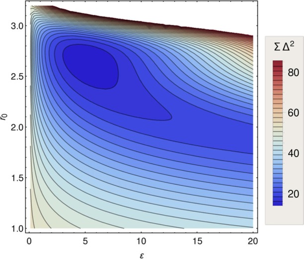
Surface of the least-squares fits (∑Δ²) of atomic LJ parameters ε and r₀ (which is σ in eq 33) for Pt(II) complexes interacting with the testing molecules. Reprinted with permission from ref (775). Copyright 2016 American Chemical Society.

4.5.1. Hybrid Model

The standard bonded model does not allow for ligand exchange processes by its very construction, while there is no such restriction for the nonbonded model. If there is a desire to have one ligand exchange, a bonded/nonbonded hybrid model can be employed. However, the VDW parameters of the metal ion or ligating atoms may need to be adjusted when using this strategy. This is because the nonbonded model assumes an integral charge, which is equal to its oxidation state, but the bonded model usually uses partial (nonintegral) charges obtained using ESP or RESP fitting protocol. Because the partial charge on a metal ion is usually less than its oxidation state, this may result in an underestimation of the interactions between the central metal ion and its ligating residues represented by the nonbonded model. For instance, Lin and Wang have tested the nonbonded model using RESP charges on the metal site. They found the central zinc ion “escaped” the metal binding site rapidly during MD simulation.⁶⁵⁵ In the work of Chakravorty et al. on the CusF system (a copper metallochaperone), they fine-tuned the VDW parameters of Cε3 and Cζ3 in Trp44 to reproduce the interaction between Cu⁺ and the Trp44 because the original VDW parameters underestimated the interaction strength.⁶⁵⁷

4.5.2. Physically Meaningful Lennard−Jones Parameters

As we discussed for the nonbonded model, it is essential to treat the VDW parameters within a physically meaningful range. For example, in the INTERFACE force field, Heinz et al. initially used VDW diameter parameters obtained from the literature,^776,777 while their final parametrized values usually only gave small deviations (±5%) from the literature values.⁵⁹⁸ The well depth (ε) is the most “adjustable” parameter in the LJ functional form and is related to the atomic polarizability. The INTERFACE force field was designed on the basis of the following considerations: (1) using the ε values of rare gases to determine the range of the ε parameters, as suggested by Halgren; (2) charge state considerations, where anions usually have higher polarizabilities and bigger ε values than the corresponding neutral compounds, while for cations the opposite behavior is observed; (3) volume density of the nonbonded neighbor atoms (including 1-4 interaction), whose increase usually decreases ε; and (4) a bigger ε value may be needed for some polar atoms or ions to make the LJ potential more repulsive at short-range. These nonbonded parameters were fitted to reproduce experimental bulk and interfacial properties. It was also shown that the combining rules only induce small deviations (usually below 10%) in property predictions.⁵⁹⁸ This is likely because the VDW parameters are in a physically reasonable range, which gave stable derived parameters based on different combining rules.

4.6. General Force Field Development

If there are N atom types in a force field, the bond, angle, and dihedral terms approximately scale as O(N²), O(N³), and O(N⁴), respectively. With more than 100 elements in the periodic table and with the potential for multiple atom types per element (generally the more atom types in a force field, the more accurate it is), the number of parameters rapidly increases. However, it is difficult to perform parametrization for every possible bond, angle, and dihedral combinations independently. Hence, general force field models usually employ empirical rules and a simplified philosophy to facilitate the derivation of force field parameters. For example, the equilibrium bond lengths are obtained by summing the covalent bond radii of the two connected atoms combined with some corrections (e.g., offset values, electronegativity, or bond order corrections).^615,778 Bond force constants can be obtained using Badger’s rule or via another empirical relationship. The equilibrium angle values can be obtained using valence shell electron pair repulsion (VESPR) theory.⁵¹ The torsion parameters are based on the hybridizations of the two central atoms.⁶¹⁵ The VDW parameters can be obtained using experimental results such as IPs,⁷⁷⁸ or the VDW radii of noble gas atoms (through interpolation/extrapolation).⁵¹ Even though the accuracy of these force fields may be limited, these models can provide qualitative insights at minimal computational expense on a broad range of systems. Below we highlight some of the features of several general force fields.

4.6.1. Tripos 5.2 Force Field

For the sake of completeness, we describe the Tripos 5.2 force field reported by Clark et al. in 1989.⁷⁷⁹ It is a general force field designed initially for organic molecules (but offers avenues to the modeling of metal systems) and is embedded in the Sybyl program. This force field served as a prototype^397,778 for the development of generalized force fields and was designed to predict molecular geometries and relative energies. Geometry minimization was performed for a number of organic molecules (as well as crambin and several peptides), and good agreement was obtained with the available crystal structures. It is suitable for both protein and ligand simulations.

4.6.2. DREIDING Force Field

Mayo et al. created the DREIDING force field in 1990.⁶¹⁵ The equilibrium bond distances were calculated as the sum of atomic radii with an offset value. It uses the harmonic cosine equation for the angle bend term because it gives a zero slope when the angle approaches 180°. The equilibrium angle values were taken from the structures of the parent hydrides (e.g., MH₂) found in the literature.^780−783 A single Fourier equation was used for the dihedral interaction, while the 1-4 nonbonded interaction is generally left unscaled. For improper torsion interactions, they averaged over three inversion terms (eqs 100–102) for nonplanar equilibrium geometries and eq 101 for planar equilibrium geometries (when φ_I⁰ = 0°). Herein, I is the central atom and φ_I is the improper torsion angle. Simple rules were used to assign bond and angle force constants, torsion, and improper torsion terms (e.g., a bond force constant is based on the bond order times a single predefined bond force constant).

100

101

102

103

104

Either a 12-6 LJ (default) or exp-6 (X6) was used to describe the VDW interactions (see eqs 103 and 104). Here, ρ equals r_ij/r_min,ij while ε is the well depth. ζ is the scaling factor, which is dimensionless. Using ζ = 12.0, E^LJ and E^X6 have the same long-range attraction, while at ζ = 13.772 the two representations have the same behavior where the sum of VDW radii of the two particles meet. DREIDING uses an arithmetic combining rule for the VDW radii and a geometric combining rule for the well depth when using the 12-6 LJ potential. For the X6 potential, a geometric combining rule for the A and B parameters and an arithmetic combining rule for C parameters are used. Charges are ignored or determined by the Gasteiger scheme. A hydrogen-bonding potential was employed and followed a CHARMM-like style. All reported calculations were performed in a vacuum with a dielectric constant of 1. It was shown that the DERIDING force field could reproduce crystal structures, relative energies, and rotational barriers for organic molecules. Metal ion parameters were initially reported (Na⁺, Ca²⁺, Fe²⁺, and Zn²⁺ ions) for the DREIDING force field, but they were not rigorously tested in the original paper.

4.6.3. Universal Force Field

Rappé et al. reported the development of the UFF in 1992.⁷⁷⁸ It contains 126 atom types across the periodic table. The parameters were determined on the basis of general rules and are adjusted according to the element, hybridization, and connectivity of the atom types. The bond length is obtained as the sum of the atomic radii plus terms including bond order and electronegativity corrections. For the corrections, a Pauling-type bond order correction and an electronegativity correction from O’Keeffe and Brese were employed. Force constants were developed on the basis of Badger’s rules. Cosine Fourier expansions were used for the angle bending terms, which better represent large amplitude angle motions than the harmonic potential. The angle force constants were obtained on the basis of the angular generalization of Badger’s rules. Cosine Fourier expansions were employed to describe the torsion terms, while mixing rules were employed to determine the torsion barriers. Torsion interactions without a main-group element in the central bond were set to zero. The improper torsion terms were represented by cosine Fourier expansions containing one or two terms. The 12-6 LJ potential with geometric combining rules were used for both the VDW radii and the well depth. These parameters were derived by initially fitting experimental data to the exp-6 expression, and subsequently the 12-6 LJ values were derived using the mathematical relationship between the 12-6 LJ and exp-6 equations. Point charges were derived on the basis of the EEM (so-called FQ model, see section 6.1). A number of tests were performed with several TM complexes. In general, it was shown the UFF reproduced bond distances within ±0.1 Å and angles within ±5° to ±10°.

In a separate effort, Rappé et al. applied the UFF specifically for metal complexes.⁷⁸⁴ The results support the use of the bond order correction employed in the force field. Using multiple metal-C and metal-P bond orders yielded improvement for TM-phosphine and TM-carbonyl systems where back bonding plays an important role. It was found that half-integer bond orders better account for the trans influence in metal phosphines. However, the force field showed weakness reproducing high-valent TM-π bonding systems and in systems that have strong ionic bonds (rather than covalent). Nonetheless, the authors noted that multiple bond order models are likely to better simulate the high-valent metal-π bonding effect.

4.6.4. General MM2 and MM3 Force Fields

Allinger et al. described a general approach to generate MM2 and MM3 force field parameters in 1994.⁵¹ It supported atoms from H to Hs (no. 108 in the periodic table). It uses quadratic and cubic terms to describe the bond interactions in the MM2 force field while adding quartic terms in the MM3 force field. An electronegativity correction was added to the covalent atom radii sum to represent the equilibrium bond length. For the angle terms, equilibrium angle values were obtained on the basis of the observed configurations (e.g., tetrahedral, trigonal planar, pyramidal, etc.). Second- and sixth-order terms were to model the angle interaction in MM2, while second- to sixth-order terms were employed in the MM3 force field. Torsion parameters were assigned on the basis of the hybridizations of the central two atoms. The improper torsion parameters were determined on the basis of the central atom. Bond moments, which can be obtained from earlier published work or obtained as the difference between the electronegativity of the two connected atoms, were used to represent the electrostatic interactions. The Exp-6 expression was used to represent the VDW interactions. However, almost all of the supported atom types are neutral in these force fields, and even though charged species are supported in the program, results computed for these species may need to be carefully validated.

4.7. Drawbacks of the Bonded Model

The bonded model is widely used in classical force fields. It has a simple and physically satisfying format, which leads to models that can readily simulate macromolecule systems with considerable accuracy. Despite its remarkable success, it still has several drawbacks when it comes to modeling TM containing complexes. The widely known drawback is the use of harmonic potentials for the bond and angle terms, which makes it impossible to readily simulate ligand switching or CN changes. As discussed above (see section 4.5), a hybrid model can be utilized to overcome these issues for specific ligands. A nonbonded model (see section 3), cationic dummy atom model (see section 5.1), can also be used at this point but with modest accuracy. Furthermore, reactive potentials (see section 6.5), which represent a more advanced modeling strategy, can be employed to overcome these issues.

Hu and Ryde pointed out that distorted structure occurs when modeling a structure with two or more water molecules bound to the same metal ion when using the bonded model.⁶⁷⁷ This is because 1-3 nonbonded interactions are usually not considered while the 1-4 nonbonded interactions are included in most bonded models. Because a water molecule usually has a zero VDW parameter on its hydrogen atoms, a serious problem occurs when it has two water molecules bound to the same metal ion: there will be a strong 1-4 electrostatic attraction but no 1-4 VDW repulsion between the hydrogen atoms in one water molecule and the oxygen atom in the adjacent water molecule. If the two water molecules are not on the opposite sides of the central metal ion, the attraction becomes strong enough to distort the angle. At this time, a nonbonded model with QM-derived constraints (which assigns only nonbonded interactions between the coordinated water molecules), a Urey–Bradley model (which includes the 1-3 nonbonded interaction with an added harmonic term based on the distance of the 1-3 atoms), or a reactive force field model (which includes the nonbonded interactions between each atom pair) are possible alternatives to address this problem.

The accuracy of the bonded model is also limited (see section 4.2.5), as demonstrated by Rydberg et al.⁶⁸¹ Overall, the simplicity of the model’s functional form for TMs limits its ability to reproduce some QM-derived results precisely. For instance, the bonded model uses a fixed partial charge model, which does not include POL and CT effects explicitly, but these effects are clearly important in TM-containing systems. See section 6 for a discussion on popular polarizable models currently in use.

5. Classical Modeling of Metal Ions: The Cationic Dummy Atom and the Combined Model

5.1. Cationic Dummy Atom Model

The CDAM was originally described for the Mn²⁺ ion⁷⁸⁵ and then extended to other metal ions. Now parameters are available for the Mg²⁺ and Ca²⁺ ions, as well some 3d TM ions including Mn²⁺, Fe²⁺, Co²⁺, Ni²⁺, Cu²⁺, and Zn²⁺. We are unaware of CDAM parameters for monovalent ions, which may be due to the observation that the nonbonded model is accurate enough for most situations. Moreover, to date, CDAM parameters have not been developed for highly charged ions, which is certainly an interesting future research direction for this model.

In the CDAM representation shown in Figure 57, there are six dummy sites connected to the central metal ion. The number of dummy sites can vary according to the CN of the metal ion being studied. The equilibrium bond distances between the metal ion and the dummy sites are usually set at 0.9 Å (with the exception of the Cu²⁺ ion, see below). The dummy sites have fractional masses, while the total mass of the central nucleus and its associated dummy sites is equal to the mass of the ion, with the total charge of metal ion and its allied dummy sites summing to the formal charge of the ion. To reproduce experimental HFEs, the charge of the central nuclei can hold a negative charge enhancing the positive charges on the dummy sites. The charges of the dummy sites are set equal to each other except for the Cu²⁺ ion (to reproduce the Jahn–Teller effect). VDW parameters were not assigned to the dummy sites initially, while in recent work a small repulsive term has been introduced. It has been shown that CDAM simultaneously reproduces experimental HFE and IOD values, thereby offering an improvement over nonbonded models.⁷⁸⁷ However, even though CDAM has more atom sites, this does not guarantee that better results will always be obtained over the standard (12-6 LJ) nonbonded model for ions.⁷⁸⁸ The nonbonded model assigns an integral charge to the metal ion, while the CDAM approach assigns fractional charges to the dummy sites, which may decrease the interaction strength between the ion and specific residues.⁷⁸⁸ Moreover, the negative charge on the nucleus clouds the physical meaning of the model, which in turn hampers its predictive ability. Meanwhile, because an assumed CN is assigned to the ion, the CDAM may not be able to simulate processes involving CN changes. Nonetheless, whether to use the traditional nonbonded or CDAM comes down to the quality of the parameter sets used in the evaluation process.

Figure 57.

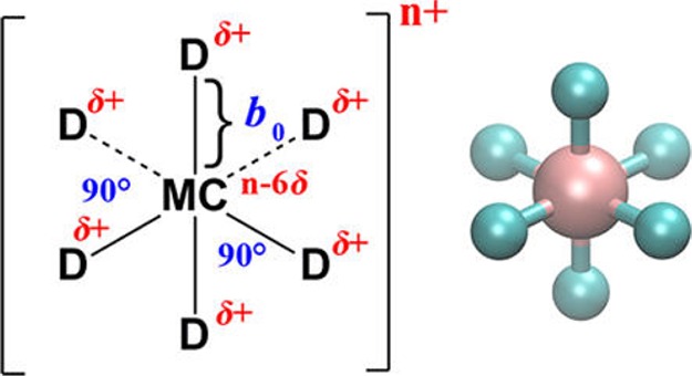
Geometry of the cationic dummy atom model with octehdral shape and a charge of n+, in which the central metal ion with a charge of n – 6δ bonds covalently to six dummy sites each with a charge of +δ. Reprinted with permission from ref (786). Copyright 2016 American Chemical Society.

Åqvist and Warshel investigated metal ion substitution effects on the activation energy of catalysis by staphylococcal nuclease (SNase) using the EVB approach.⁷⁸⁵ In their work, they parametrized the Mg²⁺, Sr²⁺, and Ba²⁺ ions using the 12-6 LJ nonbonded model to reproduce the experimental relative HFEs to the Ca²⁺ ion and the first peak of the metal ion-oxygen RDFs. Their results showed that all three of the ions increase the activation energies over Ca²⁺, implicating Ca²⁺ as the optimal catalytic ion for SNase. The predicted trends agreed well with the available experimental results. As an outcome of this effort, they found that it was hard to reproduce the relative HFE and RDF for the Mn²⁺ ion simultaneously. To address this issue, they introduced CDAM to model the Mn²⁺ ion. The model consists of a central site with charge (−0.1e) and VDW parameters, connected to six octahedrally coordinated dummy sites each with a charge of +0.35e, yielding a total charge of +2e. It was shown that the model reproduced the relative HFE to Ca²⁺ as well as a RDF consistent with its ionic radius. They proposed that the crystal field stabilization energies of the TM ions yield more negative HFE values than seen for “spherical” ions that have similar radii. They also discussed that based on ligand field theory, the electron density of the central ion would partly shift to the d orbitals along the bisectors of the ligands, which decreases the shielding effect and causes stronger interactions with ligands than seen in “spherical” ions. They also note that simulating divalent ions is more difficult than for monovalent ions largely due to their higher HFEs. The calculated activation energy for the reaction with Mn²⁺ is ∼6 kcal/mol higher than that of Ca²⁺, which agreed well with the experimental kinetic results that indicate that the reaction using Mn²⁺ is at least 36 000 times less efficient than the one using Ca²⁺. It is impressive that good agreement could be obtained with experimental data based on these simple models. Moreover, they had an insightful discussion about the catalytic mechanism of enzymes similar to SNase in the work.

105

The upper part of Figure 58 shows the free energy changes of the proton-transfer reaction (see eq 105) for different combinations of B (base) and M (catalytic metal ion). The lower part of Figure 58 shows enzyme examples, indicating the effect that the presence of metal ion has on the reaction free energy. For example, the presence of a zinc ion decreases the free energy of reaction from 21 to 13 kcal/mol for the transfer of a proton to a water molecule (like the situation in carbonic anhydrase).

Figure 58.

(a) Diagram showing the effects of metal ion and general-base catalysts on the reaction of eq 105. The abscissa denotes increasing general-base strength, represented by a water molecule, a carboxylate ion, and an imidazole ring. The ordinate represents increasing metal ion electrophilicity, where a water molecule denotes the case where no metal is present. The energy values, ΔG_ij, correspond to the proton-transfer reaction (M²⁺_i)H₂O + B_j ⇌ (M²⁺_i)OH^– + BH⁺_j, where each entry is obtained from ΔG_ij = −2.3RT(pK_j – pK_i). For example, in the case of a metalloenzyme using Ca²⁺ and glutamate, respectively, as M and B, i denotes Ca²⁺(H₂O) and j denotes (Glu)-COOH (the pK_a’s for metal bound water are taken from ref (789)). (b) The figure shows a number of different enzymes that catalyze reactions involving a proton-transfer step like eq 105, plotted according to their use of metal ion and general-base catalysis (SNase, DNase I, and RNase denote staphylococcal nuclease, deoxyribonuclease I, and ribonucleases [e.g., A and T₁], respectively). Reprinted with permission from ref (785). Copyright 1990 American Chemical Society.

CDAM parameters have been developed for the Zn²⁺ ion, and the resultant parameters were applied to a study of human carbonic anhydrase I (HCAI) using the EVB approach.⁷⁹⁰ Six dummy atom sites were used in the model with each having a +0.5e charge. The derived parameters reproduced both experimental HFE and IOD values. The simulated results agreed well with experimental data and indicated the importance of electrostatic interactions related to the catalytic Zn²⁺ ion.

Oelschlaeger et al. parametrized the CDAM for Mg²⁺ and applied the parameters to a study of Human DNA polymerase β.⁷⁹¹ The target values they used were the HFE together with QM calculated energies and structures. They assigned a mass of 3.0 amu to each dummy site, which did not have VDW interactions. The central nucleus was assigned a charge of −1.0e, while each dummy site was assigned a charge of +0.5e. It was shown that the CDAM better represented the structures and energies of the Michaelis and transition state complexes than the traditional nonbonded model.

Saxena and Sept parametrized CDAM for Ca²⁺ and Mg²⁺ ions.⁷⁹² Because the most common geometry for Ca²⁺ sites in biological systems is the pentagonal bipyramid, they placed 7 dummy sites around the central nuclei (see Figure 59), while an octahedral geometry was used for the Mg²⁺ ion. The central nucleus was treated as neutral and the dummy sites had uniform charges. The parametrization effort targeted the reproduction of experimental HFEs, but was also found to be able to reproduce experimental RDFs. By calculating relative binding energies of Mg²⁺ and Ca²⁺ to different systems, it was shown that the CDAM model outperformed all tested nonbonded models. In a related effort, Saxena and García refined the original CDAM parameters for Mg²⁺ and Ca²⁺.⁷⁹³ This was done because the initial parameter set could not simulate solutions with high salt concentrations (see sections 3 and 6 for further discussion on this point). They fine-tuned the C₁₂ parameter between the dummy atom sites and the Cl^– ion without influencing the interaction between the nuclei or dummy sites with water molecules. The C₁₂ parameter was refitted to reproduce experimental osmotic pressures of MgCl₂ solutions at different concentrations. It was shown that the new parameter set eliminated artifacts associated with ion aggregation seen with the original parameter set. The new parameter set also reproduced the experimental osmotic pressure values of CaCl₂ solutions, demonstrating their excellent transferability.

Figure 59.

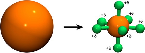
Illustration of the multisite ion model for calcium in the study of Saxena and Sept.⁷⁹² Instead of a simple sphere, the charge centers are now distributed to multiple sites depending on the coordination geometry of the ion. Reprinted with permission from ref (792). Copyright 2013 American Chemical Society.

Duarte et al. developed CDAM parameters for Mg²⁺, Ca²⁺, Mn²⁺, Fe²⁺, Co²⁺, Ni²⁺, and Zn²⁺ ions.⁷⁸⁷ All of these models used an octahedral geometry with every nuclei assigned with a −1.0e charge and every dummy site assigned a +0.5e charge. The experimental HFE and IOD values were the parametrization targets. It was shown that the resultant parameter sets reproduced both values simultaneously. Tests on metal-containing enzyme systems also demonstrated the stability of the parameter set.

Liao et al. developed a CDAM model for the Cu²⁺ ion, which incorporated the Jahn–Teller effect.⁷⁹⁴ They found that by assigning larger charges to the equatorial dummy sites, they were better able to simulate the Jahn–Teller effect. Intriguingly, along with the uneven charge assignment, they found the “compressed” octahedral structure performed better than a symmetrical or elongated octahedral environment. They arrived at final charges for the axial and equatorial dummy sites of +0.05e and +0.725e (with the metal core assigned a charge of −1) and axial and equatorial bond lengths of 0.8 and 1.0 Å, respectively. The higher charges on the equatorial sites were also helpful in reproducing the square-planar structure of four-coordinated Cu²⁺. The final parameter set was able to reproduce the experimental HFE and IODs (both of two different Cu–O distances due to the Jahn–Teller effect) simultaneously and performed well on two different copper-containing enzyme systems.

Lu et al. performed simulations on glycogen synthase kinase 3β (GSK3β),⁷⁸⁸ which has two Mg²⁺ ions in two different sites that serve as cofactors to catalyze the process of γ-phosphate transfer from ATP to the Ser and Thr residues in the substrate. They studied the parent system and one system in which the Mg²⁺ ion in site 1 is substituted by a Ca²⁺ ion. They found that the Mg²⁺ ion nonbonded model outperformed the CDAM one based on two 20 ns simulations on the parent system. The CDAM model distorted coordination modes for the two Mg²⁺ ions, and disrupted an important hydrogen bond in the active site, while the nonbonded model better reproduce the XRD determined active site structure, even though the CDAM model offered closer metal–oxygen coordination distances when compared to the X-ray structure.

Pang et al. performed a series of studies applying the CDAM approach to zinc-containing metalloproteins.^795−801 Herein, we show an example of the extensive work carried out by them. Peng developed a tetrahedrally coordinated CDAM for the Zn²⁺ ion in 1999.⁷⁹⁵ The nucleus was treated as neutral, while the +2e total charge was assigned to four dummy sites (each has a 0.1 amu mass) equally, to mimic the 4s4p³ empty orbitals. There is no VDW interaction assigned to the dummy sites. This CDAM model was developed to decrease the underestimation of ion–water interactions in the nonbonded model. Their resultant CDAM model predicted shorter Zn–S distances than experimental data, but it significantly improved the prediction of the HFE value (as −448 kcal/mol, ∼8% smaller than experiment). It was also shown the CDAM model better reproduced the interaction energy of the Zn²⁺–water dimer than the nonbonded model. Tests carried out on carboxypeptidase, carbonic anhydrase II, and rubredoxin demonstrated the stability of their CDAM model. Besides these systems, they have also applied the CDAM model to study farnesyltransferase,⁷⁹⁶ phosphotriesterase,⁷⁹⁷ and endopeptidase.^798−801

Recently, Jiang et al. refined the Mg²⁺ parameters of the CDAM model for TIP3P water through a simple parameter screening strategy.⁸⁰² A revised experimental HFE value was used, and an energy correction protocol was employed to improve the parameters’ transferability among different simulation strategies. The new parameters reproduced both thermodynamic and structural properties, and it offered improvement over previously developed nonbonded models from Åqvist and Allner, as well as the CDAMs from Oelschlaeger and Duarte, in terms of reproducing the ATP/GTP-Mg²⁺-protein environment in three metalloenzymes (where the metal center has one or two ions). However, the new model failed to reproduce the Mg²⁺–Mg²⁺ distance and was biased toward monodentate binding to carboxylate groups. Use of a bonded model was suggested to diminish these artifacts. Following this work, Jiang et al. systematically parametrized 11 6-coordinated divalent metal ions for the TIP3P, SPC/E, and TIP4P_EW water models.⁷⁸⁶ The experimental HFEs for the ions were obtained by assigning the HFE of the proton as −265.9 kcal/mol. A negative charge of −1.0e or −2.2e was assigned to the atomic cores of these divalent metal ions, while 0.9–1.3 Å bond lengths were used for the bonds between atomic core and the dummy atomic sites. An energy correction protocol was also employed in this work, and the final parameter sets reproduced experimental HFE, IOD, and CN values simultaneously.

5.2. Combined Model

As shown in Figure 60, the combined model considers the ion and its first solvation shell as a unified unit in the molecular modeling process.⁸⁰³ Because of this, simulating water exchange in the first solvation shell is not possible. This representation is reasonable for highly charged ions under relatively short simulation time scales because of the long MRT of first solvation shell waters. Typically the parametrization is based on appropriate quantum calculations. To date, there are combined models for main group ions such as Be²⁺,⁸⁰⁴ Mg²⁺,⁸⁰⁴ and Al³⁺,^804,805 TM ions including Cr³⁺,^{803,806−809} Zn²⁺,^810−812 Cu²⁺,⁴⁴ Pd²⁺,^813,814 and Pt²⁺,⁸¹⁴ and even the Th⁴⁺ ion.⁸¹⁵ The combined model, by its very design, incorporates many-body effects (e.g., CT and POL effects) in the first solvation shell directly and addresses the (potential) electronic state crossing problem. In the early development of the combined model, the hydrating ions were treated as rigid,^807,810 while in subsequent work intramolecular potentials for the hydrated ion were also added to construct flexible models.^805,809 However, because it is usually parametrized using QM calculated results, the accuracy of the resultant potential will be directly influenced by the accuracy of the QM computations. Marcos, Martinez, and co-workers have done a series of related work on the combined model, and, herein, we explore several examples.

Figure 60.

Structure of the minimum corresponding to 12 water molecules interacting with the Cr³⁺ hydrate using the HIW_P and the MCHO potentials in the study of Martínez et al.⁸⁰³ Drawn bonds between the cation and oxygens of the first-shell water molecules represent the feature of the HIW_P to consider the hydrate as a single unit. Reprinted with permission from ref (803). Copyright 2000 American Institute of Physics Publishing LLC.

The first combined model of an ion was proposed by Pappalardo and Marcos.⁸¹⁰ They fitted a potential for the Zn²⁺ hydrate ion based on QM calculations. They obtained a hydration energy for Zn²⁺ of −517.6 kcal/mol based on the combined model, which is much closer to the experimental value of −491 kcal/mol, than the values based on a two-body conventional potential (−844.6 kcal/mol) and on a potential that included three-body corrections (−848 kcal/mol). They found that water molecules in the second shell have less directionality when employing the combined model than when using a nonbonded model. They proposed that the use of a flexible water model could reduce the extent of this exaggeration in the second shell of water molecules. Later, they performed a series of simulations that demonstrated that the difference between the hydration energy predicted by their model and that from the Clementi potential is mainly due to differences in the ion–water interaction.⁸¹⁶ The latter model overestimated the ion–water interactions, yielding a too negative hydration energy. Results also showed that geometric relaxation caused only limited (∼2.5%) changes in the hydration energy. As another benefit, they proposed that the combined model better incorporates long-range interactions.

Martínez et al. described a fully flexible combined model for the Cr³⁺ ion⁸⁰⁹ in which an intramolecular interaction potential was used to represent the interaction between the Cr³⁺ ion and its first solvation shell waters. The potential was fit on the basis of a QM-derived PES between Cr(H₂O)₅³⁺ and H₂O. CHELPG charges were assigned to all of the atoms, and LJ parameters from the TIP4P water were used to describe the VDW interaction between the first solvation shell water molecules. A 4-6-12 potential (between Cr³⁺ and the oxygen atoms in the first solvation shell) was used to describe the interaction (except electrostatic) between Cr³⁺ and its first solvation shell water molecules. It was found that the C₄ term was negative, while both the C₆ and the C₁₂ were positive. The TIP4P water model was used for the remaining water molecules. The potential between the hydrated ion and other water molecules was taken from related work.⁸⁰⁷ It is noted that this fully flexible model can be treated as a nonbonded model (but the parameters of the first solvation shell water molecules and bulk water molecules are different) because there are no bonded terms for the intramolecular interactions between the Cr³⁺ ion and its first solvation shell water molecules. Because of the high charge on the Cr³⁺ ion (+2.457e, based on the CHELPG algorithm), it is unlikely that exchange of the first solvation shell water molecules happens during the routine MD time scale nowadays. It was shown that a 4-6-7 potential offered improved performance over the 4-6-12 potential in the reproduction of intermolecular vibrational frequencies. Their results showed that the flexible model gave dynamics properties similar to those of the earlier rigid model. The results also support a proposed definition of the hydrated ion that suggests that such an ion could be considered as “hydrated” if its rotational motion obeys the Debye rotational model.

6. Classical Modeling of Metal Ions: The Polarizable Model

The importance of the polarization effect has been discussed in detail for some years.^158,159,162 For example, according to symmetry adapted perturbation theory (SAPT) theory, the polarization energy can range from very small to values around 10–20% for the total interaction energy.⁸¹⁷ It has been shown that the polarization effect becomes more pronounced in highly charged systems, where the electronic cloud is more polarized.³⁹¹ Furthermore, the polarization effect is also important in hydrogen-bond formation, cation−π interactions, and receptor–ligand recognition. The polarization effect can be qualitatively represented using overpolarized charge parameters within an unpolarized two-body model, but it is still hard to simulate the charge delocalization effect accurately by using the classical additive potentials. This is because that the polarization effect becomes nonadditive when there are more than two molecules in the system.¹⁵⁹

In unpolarized models, the charge distribution is fixed, and two identical amino acids, but in different environments, are assigned the same charge parameters. This is not particularly physically meaningful because surrounding particles influence their charge distributions. This kind of difference can be considerable, for example, between an amino acid in a buried site versus that on the protein surface. Unlike unpolarized models, polarizable models allow the electronic distribution to change, which allows inclusion of the charge delocalization effect in response to the environmental changes. This facilitates the polarizable model’s ability to reproduce both gas- and liquid-phase properties simultaneously. For example, it is hard to model gas-phase properties of water using typical unpolarized water models because of the overestimation of the polarization effect. The water dimer energy predicted by the TIP3P water model is −6.5 kcal/mol, while many polarizable water models yield values close to −5.0 kcal/mol, an accepted value predicted by QM modeling.¹⁶⁷

There are three basic types of polarizable models in common usage: the FQ model, the DO model, and the induced dipole model (IDM). Meanwhile, there are also three ways to propagate simulations using polarizable force fields: self-consistent field (SCF), matrix inversion, and extended Lagrangian methods. To help conserve energy, smaller time-steps may be needed during simulations using polarizable models relative to unpolarized ones. Early on, the SCF method was used to propagate MD simulations using polarizable models.^818−820 It performs an energy minimization inside each time-step until converge is reached; however, multiple steps are needed to converge inside each time-step increasing the cost. Besides the SCF method, the matrix inversion method can be used.^821−823 However, inversion of a large matrix representing a macromolecule is time-consuming. Recently, the extended Lagrangian method^824−827 has become the preferred method for MD simulation with polarizable force fields due to its reduced computational cost and good accuracy. It traces its origins to the CPMD approach and includes a polarizable degree of freedom into the dynamics.³⁶⁷ For example, similar to CPMD simulations, a fictitious charge mass (energy·time²/charge²) can be employed in the FQ model.⁸²⁸ However, in the Lagrangian method, extra works usually need to be performed to assign proper weights to the pseudo particles (e.g., Drude particles), use, and fine-tune two separate thermostats for atoms and pseudo particles. To date, polarizable models have been developed for metal ions with s, p, d, and f orbitals.

6.1. Fluctuating Charge Model

6.1.1. Model Introduction

The FQ model is one of the simplest polarizable models extant. Even though it utilizes a point monopole representation, it still allows charge fluctuation on the basis of changes in the chemical environment. It uses a Taylor expansion of the atomic chemical potential up to second-order terms in atomic charges. Many FQ models have been developed, including the EEM,^829−832 OPLS-AA-FQ,⁸³³ CHARMM-FQ,^828,834 the ABEEM/MM model,^835−852 etc. These models are generally based on the CPE scheme. Dipole moments are usually overestimated in the FQ model,⁸²⁸ and artifacts are observed if CT is allowed between far distant atoms. Hence, to make this approach work effectively for macromolecules, extra constraints are applied to alleviate these problems.^166,167 Along with these issues, the FQ model has difficulties in simulating out-of-plane polarizabilities.¹⁶⁶ The FQ method is much faster (by several orders of magnitude) than ab initio or DFT methods, while still generating reliable partial charges for a range of chemical compounds. This opens a range of applications involving screening or filtering compounds.⁷⁷²

6.1.2. Historical Development

Jensen has discussed the origin and development of the electronegativity concept from its early stage.^853,854 In 1932, Hund proposed that if two atoms have equal (E_IP + E_EA)/2 values, they could be treated as having an approximately equal contribution to the bond formation between them.⁸⁵⁵ Pauling proposed the electronegativity concept in 1932,⁸⁵⁶ which was used to represent the relative attraction of valence electrons for each atom in a covalent bond. He calculated atomic electronegativity values on the basis of experimental bond energies. The square of the electronegativity difference between two elements A and B was determined using (χ_A − χ_B)² = ΔE_AB^bond = E_AB − (E_AA^bond + E_BB)/2.

Later, Mulliken defined the “absolute” electronegativity scale on the basis of an average of the IP and EA, and obtained values in agreement with Pauling’s data.⁸⁵⁷ He proposed that when A and B have equal electronegativities, the difference between the two states A⁺B^– and A^–B⁺ can be neglected, yielding IP_A – EA_B = IP_B – EA_A, so IP_A + EA_A = IP_B + EA_B. So IP_A + EA_A or (IP_A + EA_A)/2 can be used to define the absolute electronegativity.

Sanderson proposed the seminal concept of electronegativity equilibration in the early 1950s.⁸⁵⁸ He proposed that when two atoms approach one another to form a bond, the one with the larger electronegativity attracts more electrons. This increases its atomic radius and decreases its attraction to valence electrons. The opposite occurs for the atom with the smaller electronegativity. This process will adjust the radii of the two atoms to equalize their electronegativity, and the final bond length equals the sum of the adjusted radii. He then proposed the stability ratio function as a measure of the electronegativity. The effective radii of atoms can then be obtained using eq 106:

106

107

As shown in eq 107, ED is the average electronic density (in units of electron/ų), while r represents the nonpolar covalent or ionic radius. In eq 106, ED_i is the average electronic density of the corresponding noble gas atom (representing the maximum inertness of an atom), and SR_m is the stability ratio ED/ED_i in the molecule, which represents the chemical reactivity or electronegativity of a particle that has the same electron count as the corresponding noble gas atom.⁸⁵⁸ The bond length is the sum of the effective atomic radii of two connecting atoms. The calculated bond lengths based on this model agreed well with experimental results: the mean deviation was 0.05 Å for 95% of the bonds explored. In a later publication, calculations on alkaline halogen compounds were performed.⁸⁵⁹ Even though these are highly polarized systems and their bond length is usually less than their sum of covalent radii, Sanderson showed that the calculated results agreed well with experimental data. Slight improvement in the modeling was obtained by using ionic instead of covalent radii.

In 1978, Parr and co-workers proposed that electronegativity equals the negative of the chemical potential for the ground state, based on the viewpoint of DFT.⁸⁶⁰ They showed that the energy determines the chemical bond formation, while the electronegativity difference determines whether CT occurs upon bond formation. This proved the assumption of Sanderson. Subsequently, Parr and Pearson proposed the concept of chemical hardness and defined its formulation.⁸⁶¹ It is defined as the second derivative of the energy with respect to the number of electrons in the system, thereby representing the resistance of the chemical potential to changes in the number of electrons. This quantity can be directly calculated on the basis of the finite difference formula . It represents one-half of the energy needed for the following process to occur: A + A → A⁺ + A^–. They also laid the theoretical framework of the hard soft acid base (HSAB) principle based on the concepts of electronegativity and chemical hardness. Reasonable results were obtained from their calculations on chemical hardnesses for a number of atoms, ions, and compounds.

Hinze et al. proposed the concept of orbital and bond electronegativities in the early 1960s.^862−865 Years later, Gasteiger and Marsili developed the partial equalization of orbital electronegativity (PEOE) charge (so-called Gasteiger charges).^866,867 This was followed by the work of Mortier et al., who developed the electronegativity equalization method (EEM) for the determination of atomic charges.⁸²⁹ Rappé and Goddard described the charge equilibration (QEq) approach⁸⁶⁸ and applied it to the UFF.^{778,784,869,870}

6.1.3. Formulation of the Fluctuating Charge Method

It is noted that different FQ methods may have subtle differences in formulation and implementation. Herein, we treated the QEq method as an example. Formally, the QEq method proceeds as follows:

108

109

110

111

112

113

where

114

115

116

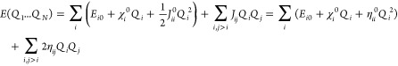117

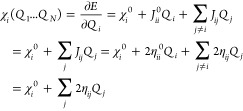118

Herein, the χ⁰ and η⁰ are the electronegativity and chemical hardness (which is related to the Hubbard U parameter) parameters, respectively. Here, we assume J_ij = J_ii⁰. The constraints used in solving the equations are (1) the electronegativity values of all atoms in the system are the same (eq 119) and (2) the total charge is conserved (eq 120).

119

120

In total, there are N equations and N variables. The charge distribution is approximated via the solution of these linear equations.

The typical FQ model does not describe the bond formation/dissociation process well, while the split charge equilibration (SQE)^871,872 and the atom-condensed Kohn–Shan DFT approximated to second-order (ACKS2)⁸⁷³ methods offer improvements.

In the FQ model, the electrostatic and electronegativity terms facilitate charge separation, while the chemical hardness term is a damping term in opposition. The electronegativity and chemical hardness parameters can be determined using QM calculations, extracted from experimental data, or treated as empirical parameters. Patel and Brooks proposed the following relationship between the polarizability tensor and chemical hardness matrix elements, thereby bridging between the FQ model and the IDM:⁸²⁸

121

Here, the Δr̅ is the atomic coordinates relative to the geometric center, based on which one can derive parameters for the chemical hardness or values for the polarizability.

6.1.4. Studies of Berne and Co-workers

Rick et al. developed FQ versions of the SPC and TIP4P water models (the SPC-FQ and TIP4P-FQ models).⁸⁷⁴ The FQ models outperformed their unpolarized counterparts. By employing the extended Lagrangian method, the new models only had a modest increase in computational cost (∼10%) over the unpolarized models.

Stuart and Berne explored the Cl^– ion in aqueous solutions using a mixed polarizable model (with TIP4P-FQ model for water and a DO model for the Cl^– ion), and compared it to an unpolarized model.⁸⁷⁵ They observed that the Cl^– ion prefers to localize near the air–liquid interface in water clusters of varying size (up to 255 water molecules) when using the polarizable force field. However, this phenomenon was not observed in simulations using an unpolarized model. They proposed that this might be because the fluctuating dipole of the water molecules allowed them to remain mobile while the polarizability of the Cl^– played a lesser role. They then went on to investigate surface curvature effects in aqueous systems with Cl^– using the same polarizable model.⁸⁷⁶ The results showed that the solvation depth profile is dependent on the interface curvature, which agrees with the “structure-breaking” behavior of the Cl^– ion.

6.1.5. ABEEM Model

Yang and co-workers have developed the ABEEM model and validated it on several large molecules.⁸³⁵ It places charges on both atoms and bonds, with the positions of charges on the bonds based on the covalent radii ratio of the two connected atoms. They have performed the model parametrization based on QM calculations on over 100 molecules.⁸³⁵ Tests were carried out on several large organic molecules, and the obtained results agreed well with QM-derived results. They followed this up with the ABEEM-7P water model.⁸⁴⁰ It uses a flexible representation for the water molecule, places VDW interactions, not only on the oxygen atom, but also on the hydrogen atoms, and has an independent parameter that describes the hydrogen-bond interaction. The ABEEM-7P water model was shown to reproduce the properties of water clusters (including 2–6 water molecules).⁸⁴⁰ A subsequent study was performed to examine the energetic, structural, and dynamic properties of the ABEEM-7P water model in the liquid phase under different temperatures.⁸³⁹ Overall, it was shown that the calculated properties agreed well with experimental observations.

Li and Yang studied Li⁺(H₂O)_n (with n = 1–6 and 8) clusters using the ABEEM/MM model.⁸⁴¹ The ABEEM-7P water model was used in the modeling. Parameters related to Li⁺ were fitted to QM and experimental data on Li⁺(H₂O)_n clusters. Charge constraints were placed on the Li⁺ and its first solvation shell water molecules, while a neutrality constraint was used for each water molecule beyond the first hydration shell. The model predicted geometries, binding energies, and vibrational frequencies that agreed well with experimental and QM-derived data. They also performed MD simulations on the Li⁺-aqueous system based on the ABEEM/MM model.⁸⁴² They calculated RDFs, DCs, and residence times of solvated water molecules in the first solvation shell at different temperatures (in the range of 248–368 K). Their reported results agreed well with available experimental data, and it was also shown that the ABEEM/MM model outperformed available unpolarized models.

Yang and Li have studied solvated monovalent ion systems (both as ionic clusters and as ion-aqueous systems) using the ABEEM/MM force field.⁸⁴³ The investigated systems contain Li⁺, Na⁺, K⁺, F^–, Cl^–, and Br^–, and they studied ionic clusters containing 1–6 water molecules. It was shown that the parameters derived for small clusters were transferrable to the liquid phase. The ABEEM/MM force field was able to reproduce both ionic clusters and liquid properties simultaneously. In subsequent research on ionic clusters and solutions of divalent ions (Be²⁺, Mg²⁺, and Ca²⁺),⁸⁴⁴ they fit the electronegativity, chemical hardness, and VDW parameters using QM calculations on ion–water clusters. MD and FEP approaches were employed to simulate different properties of these ion-aqueous systems. A charge constraint was applied to the ion and its first solvation shell water molecules, while the remaining water molecules were constrained to individually have a net zero charge. Generally the ABEEM/MM force field yielded results in agreement with QM and experimental data. However, the CN for the Be²⁺ ion was overestimated, implying a more sophisticated potential will be needed to better model this system.

Continuing their research theme, Yang and Cui fit the electronegativity and chemical hardness parameters of 3d TMs in the ABEEM force field.⁸⁴⁸ The target atomic charges, which they tried to reproduce, were obtained on the basis of Mulliken analyses at the B3LYP/6-31G* level of theory. More than 300 organometallic compounds were contained in the training set. As shown in Figures 61 and 62, even though the absolute values were not close, the final derived electronegativity and chemical hardness parameters follow the trend of experimentally determined values. Further tests were carried out on several large biorelated organometallic compounds, and good agreement was obtained with the B3LYP/6-31G*-derived Mulliken charges. In a subsequent work, Cui et al. parametrized the ABEEM/MM model for the heme group.⁸⁴⁹ It was shown that through a better consideration of the charge delocalization effect, the ABEEM/MM model outperformed the unpolarized CHARMM force field in reproducing crystal structures.

Figure 61.

Correlation diagram between the absolute electronegativity parameters and the ABEEM parameters χ* for some metal ions. Reprinted with permission from ref (848). Copyright 2007 American Chemical Society.

Figure 62.

Correlation diagram between the absolute hardness parameters and the ABEEM parameters 2η* for some metal ions. Reprinted with permission from ref (848). Copyright 2007 American Chemical Society.

Further extending their work on TMs, Yang et al. fit the reference charge, electronegativity, and chemical hardness parameters for 3d, 4d, and 5d TMs in the ABEEMσπ force field.⁸⁵² More than 700 structures were contained in the training set. The target values were the Mulliken charges obtained at the HF/STO-3G (for 3d and 4d TM complexes) or HF/CEP-4G (for 5d TM complexes) level of theory, and the dipole moments calculated using larger basis sets. It was argued that smaller basis sets give a more reliable prediction of partial charges in these systems, while bigger basis sets may overestimate these values. It was shown that the ABEEMσπ force field, which fit parameters as described above, showed much better agreement with dipole moments calculated at the HF/6-311+G(d,p) level of theory than those based on the HF/STO-3G level of theory. Finally, 5 Mo⁴⁺ ion-containing metalloproteins were minimized using the ABEEMσπ force field, and the structures obtained agreed with the available PDB structures.

Comba et al. have parametrized a FQ model (other than the ABEEM model) for complexes containing Fe²⁺ (low-spin and high-spin), Fe³⁺ (low-spin and high-spin), Co³⁺ (low-spin), and Cu²⁺ ions.⁸⁷⁷ Spectroscopy data from the National Institute of Standards and Technology (NIST) were used to generate the isolated atom parameters through a quadratic fitting strategy. Four training sets with 96 structures in total were used to fit the electronegativity and chemical hardness parameters. These parameters were fit to reproduce the reference charges using an iterative Hirshfeld method coupled with the B3LYP/6-31G* or B3LYP/TZVP level of theory. Ultimately, atomic charges were calculated for a test set containing 13 structures based on the FQ model, and the obtained values agreed well with QM calculated charges generated by the iterative Hirshfeld method. Afterward, Comba et al. applied this FQ model to the ⁶⁴Cu complexes in a quantitative structure–activity relationship (QSPR) related study for the lipophilicity predictions.⁸⁷⁸

6.1.6. Periodic Systems

Besides FQ models developed for nonperiodic TM complexes, there are also examples of FQ models developed for periodic metal-containing systems. There are numerous examples of periodic systems that we would like to model using classic methods, but given their sizes how to assemble their charge distributions is a challenge. The FQ model offers some respite to this problem, and in what follows we give some examples of this approach.

Ramachandran et al. created the periodic charge equilibration (PQEq) method to derive the charges for periodic systems.⁸⁷⁹ They applied the method to systems related to zeolite Y and found that the zeolite lattice has little influence on the charge distributions of absorbed n-octane, water, and benzene, but a considerable effect on the charge distribution of the transition state in the hydride transfer reaction between the C₄H₉⁺ ion and n-octane.

Wilmer et al. proposed the EQeq method.⁷⁷² It calculates the electronegativity and chemical hardness parameters on the basis of measured IPs. The model only uses two global parameters: the dielectric strength (treated as 1.67 in this work) and a modified parameter related to hydrogen atoms, which corrects the tendency of hydrogen atoms having negative charges by assigning the IP of the neutral hydrogen atom to −2 eV instead of the experimental value of +0.754 eV.

122

The energy of the system is represented by eq 122, where E_Ck is the electrostatic energy of the kth atom interacting with the other atoms. The representation of E_Ck is different for nonperiodic and periodic systems. E_Ok is a damping function for the electrostatic interaction between two point charges with very close contact (where the point charge approximation is not yet valid). Importantly, only linear equations need to be solved making this method much faster than DFT calculations, while still offering good results in test cases involving CO₂ adsorption in MOFs.

Afterward, Martin-Noble et al. found that the EQeq method failed to predict the partial charges of TMs with high oxidation states in the amine-templated metal oxide (ATMO) complexes.⁸⁸⁰ They then added a correction term into the EQeq scheme on the basis of the relationship between the bond order and bond distance proposed by Pauling (see eq 123, where n means the bond order, r means the bond distance, with r₀ and b as two parameters; this relationship was also used in the bond valence sum (BVS) model⁸⁸¹ and CM5 charge correction⁷²³). The new method was termed as the EQeq+C method. After parametrization toward the partial charges of ATMO complexes calculated by the Hirshfeld-I (i.e., the iterative-Hirshfeld) method, and the partial charges of MOFs based on the REPEAT method, the EQeq+C method showed remarkable improvement over the original EQeq method. Transferability of the new method was also shown on a series of unrelated dipeptides.

123

6.2. Drude Oscillator and Drude Rod Models

6.2.1. Drude Oscillator Model

The DO model, which has also been called the “shell” model, was proposed by Drude in 1902.⁸⁸² As shown in Figure 63, it uses a Drude particle as the satellite particle of an atomic core to represent its induced electronic cloud. In the absence of an electric field, the Drude particle is located at the atomic core. Once the atom is placed in an electric field (E), the Drude particle will have distance d from the atomic core:

124

Figure 63.

Schemes of the DO and DR models for Au particles. Reprinted with permission from ref (884). Copyright 2008 John Wiley and Sons.

The atomic induced dipole then is treated as:

125

On the basis of the induced dipole formula, one obtains:

126

Here, α is the atomic polarizability, k_D is the force constant between the atomic core and the Drude particle, while q_D is the charge of the DO. After the system is induced by an electric field, the charge on the atomic core will change to q–q_D (where q is the total partial charge of an atom). In the DO model, both positive and negative charges can be placed on the Drude particles.

To date, DO models have been created for alkali metal, alkaline earth metal, and halide ions, as well as the Zn²⁺ and Cf³⁺ ions.^49,552,883 Among them, most of the VDW parameters are obtained by reproducing liquid-phase properties.^49,552

6.2.1.1. Early Work

Initially, the DO model was applied to ionic materials. For example, Dick and Overhauser used the Born–Mayer potential with the DO model to study crystalline systems in 1958.⁸⁸⁵ It was shown that this model could be used for the derivations of the generalizations of the Szigeti relationship, Clausius–Mossotti relationship, and the Lorenz–Lorentz relationship. It also partially explained the deviation from unity for the e*/e value from the second Szigeti relationship.^886,887 In 1959, Hanlon and Lawson applied the DO model to derive the effective charge in the Born–Szigeti equation for NaCl crystals.⁸⁸⁸ The deviation of the effective charge from the formal charge was found to be proportional to the difference between the electronic polarizabilities of the cation and anion. Moreover, results showed that the predicted dipole moments agreed semiquantitatively with experimentally observed values. In 1974, Jacucci et al. studied crystalline NaCl using the DO model⁸⁸⁹ in which only polarizabilities of the Cl^– ions were considered. The total potential was treated as the sum of the Tosi–Fumi potential and the polarization energy. DO parameters were assigned close to Sangster’s work, and other parameters from the Tosi–Fumi potential were used in the modeling. The Drude particle around the Cl^– ion was assigned a −3e charge, and the k_D value was 8.5 × 10⁵ cm^–2. Polarization only caused a ∼0.1% change in the total energy and had a small influence on the acoustic and transverse modes in the optical phonon spectrum.⁸⁸⁹ However, polarization has a large impact on the longitudinal modes, yielding improved agreement with experiment relative to an unpolarized model. Lindan and Gillan developed a new method to simulate ionic materials using the DO model, and applied it to the CaF₂ system in 1992.⁸⁹⁰ The simulation used a conjugated gradient minimization technique to obtain relaxed structures inside each MD step. They found that incorporating polarization had a limited effect on the system, and they noted that because Ca²⁺ and F^– are less polarizable ions, the observed results were not unexpected.

Mitchell and Fincham assigned fractional masses to the Drude particles, making them propagate in the same way as the atomic cores.⁸⁹¹ A smaller time-step, ∼3 times smaller than that used in unpolarized models, was necessary in their method. Their model is ∼3 times faster than the conventional DO model using the conjugate gradient relaxation approach. This is because the simulations employing the conjugated gradient relaxation approach were able to use the same time-step as employed in an unpolarized model, but needed ∼10 conjugate gradient iterations inside each time-step, which greatly increased the computational cost. They noted that when the Drude particles were assigned proper masses, the vibrational frequencies between the atomic core and the Drude particle were much higher than the lattice vibrational frequencies, allowing the new method they developed to give results similar to those of the conventional DO model, which assigned no mass to the Drude particles. They tested the new method by calculating the ion diffusion coefficients of the Na⁺ and Cl^– ions in molten NaCl and the F^– ion in superionic CaF₂, as well as by predicting phonon frequencies found in the MgO system. Good agreement was obtained when comparison was made to previous simulations based on the conventional DO model.

6.2.1.2. Recent Applications to Metal-Containing Systems

Multiple DO models have been developed for a variety of systems in recent years. Lamoureux, Roux, Mackerell, and co-workers are active in this field. They have developed DO models for water,^892,893 ions,^{49,552,894−896} small organic molecules,^897−904 amino acids,⁹⁰⁵ nucleic acids,^906,907 lipids,⁹⁰⁸ carbohydrates,⁹⁰⁹ etc. In most cases, the Drude particles were assigned to the heavy atoms. Here, we focus our review on representative work of metal-containing system modeling by the DO approach.

Lamoureux and Roux proposed a new simulation algorithm for the DO model.⁹¹⁰ They used two different thermostats on the atom core and on the Drude particle. The thermostats for the atom core and Drude particles were set to room temperature and 1 K, respectively. An extended Lagrangian algorithm instead of a SCF algorithm was used to propagate the dynamics, with the Drude particles being assigned small masses. Importantly, relatively large time-steps (1 or 2 fs) could be used with the new algorithm. A water model, which adopted the SPC geometry and added an additional Drude particle, was used in their simulations. It was shown that simulations using this algorithm and the SCF algorithm agreed in their predictions of liquid properties. Moreover, it was also shown that simulations, which used their new algorithm but employed the same thermostat on the atom centers and the Drude particles, generated less accurate results and suffered from numerical stability issues.

Lamoureux et al. described the “simple water model with four sites and Drude polarizability” (SWM4-DP) model in 2003.⁸⁹² The water model uses a rigid gas-phase geometry and placed a +q charge on each of the two hydrogen atoms, −2q on the additional dummy site along the HOH bisector, −q_D on the oxygen atom core, and +q_D on the Drude particle, which is connected to the oxygen atom, respectively. A 12-6 LJ potential was assigned to the oxygen atom core. Because of the constraints used, there were only four parameters that needed to be optimized: the distance between the oxygen atom core and its Drude particle, the polarizability of water, and the two 12-6 LJ parameters on the oxygen atom. The water model was parametrized to reproduce the properties of liquid water under different conditions, and the extended Lagrangian algorithm was used to perform the MD simulations. It was found that the water model reproduced various experimental properties (i.e., vaporization enthalpy, static dielectric constant, self-diffusion constant). However, some compromises were made during the parameter design process. For example, the polarizability of the isolated water molecule was 1.04 ų, instead of 1.44 ų obtained from experiment. They noted that this is because the “Pauli” repulsion opposes the polarizability induction. They further discussed that compromises were made for a number of reasons including the “too repulsive” nature of the 12-6 LJ potential, adopting the gas-phase geometry for condensed phase applications and the point charge representation for the short to middle range interactions. The Exp-6 potential and a smeared charge representation were suggested as possible improvements to the water model.

The SWM4-DP model was followed by the SWM4-NDP (N indicates negative) model,⁸⁹³ where a positive charge is assigned to the oxygen atom and negative charge to the Drude particle. Overall, the SWM4-DNP model is comparable to the SWM4-DP model. Highlights of the newer model were its ability to reproduce the experimental viscosity and the HFE of water, suggesting the SWM4-NDP model a suitable choice for the simulation of aqueous phase systems and dynamic processes.

Lamoureux and Roux created consistent parameter sets for the alkali and halide ions for use with the SWM4-DP water model.⁴⁹ The polarizabilities of the alkali ions were taken from earlier work, while the polarizabilities of the halide ions were scaled down by a factor 0.724 from the gas-phase ionic polarizabilities determined previously. This factor comes from the polarizability of the SWM4-NP water model divided by the experimental value of the polarizability of water. No scale factor was applied to the polarizabilities of the alkali ions because of their small magnitudes. Hence, scaled or not would have had a limited influence on the simulation results. The Drude particle charge was determined on the basis of , and the VDW parameters of the ions were fit to reproduce ion–water binding energies in gas-phase monohydrates, the HFEs of the ion pairs, and the relative HFEs of ions in the same series. The final data imply an intrinsic HFE of the proton of −247 kcal/mol (giving a real HFE of −259.45 kcal/mol, with a phase potential for the SWM4-DP water model of −12.45 kcal/mol). Even though encouraging results were obtained, the model showed less accuracy in the modeling of small ions like Li⁺ and F^–, as well as the minimized hydrates of the halide ions. Meanwhile, the limited accuracy of the LB combining rules was also discussed as an issue that limits the predictability of the model.

Yu et al. parametrized the alkali metal ions, alkaline earth metal ions, the zinc ion, and halide ions for the SWM4-NDP water model.⁵⁵² Small masses were assigned to the Drude particles (0.4 amu for each). The fitting targets they used were the total HFEs of the neutral salts and relative HFEs between ions in the same series. Monohydrate properties were also used in the parameter determination. Generally, the model simultaneously reproduced various gas-phase and liquid-phase properties obtained from experiment and QM calculations. Their data defined the real HFE of the proton as −258.8 kcal/mol (its intrinsic HFE is −246.2 kcal/mol, with an offset from the real HFE by the phase potential of −12.6 kcal/mol for the SWN4-NDP water model). The final results agreed well with the experimental HFEs of single monovalent ions from Noyes⁹¹¹ but differed substantially from some others. A Thole-like damping function between the divalent cations and water molecules was used to prevent the polarization catastrophe, which is observed when the IOD is smaller than 1.97 Å. However, the model showed less accuracy for simulating divalent cations, which may be because of the strong CT effect between these ions and the surrounding water molecules.

Archontis et al. simulated 1.2 M NaI solutions using the SWM4-DP water model and ion parameters from Lamoureux and Roux.⁹¹² A double layer was observed near the solution interface, with I^– ions closer to the surface than the Na⁺ ions. They also observed that all of the solution species near the surface have their dipole moments perpendicular to the surface, while in bulk, the dipole vectors are randomly distributed. An additional simulation was performed with an isolated I^– ion in a water slab. This showed that the induced dipole interaction plays a major role in stabilizing the I^– ion at the interface, while permanent charge-dipole interactions between the I^– ion and water molecules favor placement of I^– in bulk.

Interactions between different monovalent cations (the Li⁺, Na⁺, K⁺, and NH₄⁺ ions) and benzene along with NH₄⁺ interacting with a water molecule were studied by Orabi and Lamoureux using the DO model.⁸⁹⁴ The parameters were developed by reproduction of QM-derived results. The parameters reproduced not only the interaction energies and PESs of the cation−π dimer, but also the cooperative behavior of the cation−π–π trimers and anticooperative behavior of the π–cation−π trimers. Simulation and related analysis of the ion-benzene dimer in aqueous solution showed that the small ions Li⁺ and Na⁺ favor solvation in water, while the bigger ions K⁺ and NH₄⁺ have favorable interactions with benzene of 1.2 and 1.4 kcal/mol, respectively. Simulation of K⁺ or NH₄⁺ with two benzene molecules in aqueous solution indicated that the cation−π and π–π interactions are all enhanced when compared to those predicted with a pairwise model (the heights of the first peaks of the RDFs defining benzene–benzene and benzene–ion interactions all increased when compared to systems having one K⁺ or NH₄⁺ and one benzene in aqueous solution).⁸⁹⁴ This illustrated the cooperativity of the two different interactions in aqueous solution. This same team developed parameters for alkali ions interacting with the NH₃ molecule.⁸⁹⁵ The model was parametrized via reproduction of MP2-derived ion-NH₃ dimer properties. The resultant model reproduced the QM calculated binding energies for the M⁺(NH₃)_n (with n = 2–4) and M⁺(NH₃)_n(H₂O)_m (with n, m = 1–3 with n + m ≤ 4) systems, as well as the relative solvation free energies of these ions in ammonia. The PMFs of these ions in NH₃/H₂O mixed aqueous solutions showed Li⁺ and Na⁺ bind to NH₃ only in their second solvation shells, and K⁺ and Rb⁺ slightly favor NH₃ over water, while Cs⁺ binds to NH₃ only in its first solvation shell.

Same as with unpolarized models, balancing the parameters used to simulate mixed systems employing the DO model can pose a challenge. For instance, in the simulation of ionic solutions, one may need to optimize the VDW parameters between the counterions if ion parameters were fit for a single ion under infinite dilution conditions. For DNA in ionic solutions, one needs to balance the interactions between the counterions as well as the interactions between DNA and ions, which again can afford a challenge.

Luo et al. noted that most parametrization efforts were performed to reproduce isolated ion properties, which may not yield accurate models for the simulation of finite concentration solutions.⁸⁹⁶ To further explore this issue, they simulated NaCl and KCl solutions at different concentrations using the SWM4-NDP water model⁸⁹³ and ion parameters developed by Yu et al.⁵⁵² The osmotic pressures of KCl solutions were reproduced with only slight deviations from the experimental results for concentrations above 2 M. However, their results showed that even at 1 M, simulation of the NaCl solution underestimated the osmotic pressure. They attempted to optimize the parameters by changing the Thole-damping factors or adjusting the pairwise LJ parameters. Even though both strategies worked well to better reproduce experimental osmotic pressures, changing the Thole-damping factor, while reducing the interaction energy, did not shift the minimum position (unlike modifying the LJ parameters). It was also shown that the second virial coefficients predicted by the new parameter set were much smaller than those predicted by the original parameters, but afforded better agreement with CPMD simulation results. Overall, this work showed that examining osmotic pressure affords another route to validating computational models of ion solvation.

Galbis et al. created a DO model for the Cf³⁺ ion,⁸⁸³ in which the mobile charge densities in harmonic oscillators (MCDHO) water model⁹¹³ was used, while the atomic core and DO particle of the Cf³⁺ ion were assigned with charges of +4e and −1e, respectively. QM calculations based on two different levels of theory (MP2 and BP86) were performed but offered different CN and IOD values. Two different methods, the “Heuristic method” and “Systematic method”, were used to generate a number of geometries, and potential fits were performed on the basis of the MP2 and BP86 calculated data, respectively. Afterward, MC simulations were performed on the basis of their derived potential using the NVT ensemble. It was shown that the two obtained potentials (MP2 and BP86), which were all based on the “Systematic method”, gave similar structural results in the MC simulation, even though the MP2 and BP86 calculations showed different CN preferences. Extended X-ray absorption fine structure (EXAFS) spectra were calculated on the basis of different potentials and compared to experimental data. The results supported a CN of 8 for the Cf³⁺ ion. An analysis of the O–Cf³⁺–O angles was performed, suggesting that a square antiprism structure (for CN = 8) was preferred in the aqueous solution.

Savelyev and Mackerell balanced DO model parameters to better represent the interactions between ions, water, and DNA.⁸⁹⁶ The QM-derived data on small model molecules, experimental hydration, and osmotic properties were used as fitting targets. Partial reoptimization of the valence angle parameters in the bases, modification of the charges of select atoms in the DNA backbone, and adjustments of the LJ parameters between DNA and water as well as the LJ parameters between DNA and ions were performed to improve the model. Results showed that the new model better reproduced the ion distributions predicted by counterion condensation theory than the CHARMM36 unpolarized force field, highlighting the advantage of the DO model over the unpolarized one for the description of DNA in ionic solutions.

Besides modeling the ion–aqueous and ion–molecule systems, the DO model has also been applied to the ion-containing material systems. Herein, we introduce an example using the DO model to simulate the MOF systems. Yu et al. developed a DO model for N₂ and CO₂ molecules based on the SAPT analysis of each molecular dimer.⁹¹⁴ In total, there are four terms in the model, which are related to the exchange, electrostatic, induction, and dispersion interactions, respectively. Each term in the model was fit to the QM calculated counterpart separately. In general, the resultant force field reproduced various properties of gaseous N₂ and CO₂ as compared to experimental data. On the basis of this work, McDaniel and Schmidt created the ZIF FF to simulate CO₂ and N₂ adsorption in the ZIF systems.⁹¹⁵ An extension of the Williams–Stone method was used to represent the dispersion interactions and was able to accurately reproduce the calculated dispersion energies on the basis of the SAPT theory. Simulated CO₂ and N₂ adsorption isotherms for nine different ZIFs agreed well with the available experimental data. Results implied that UFF overpredicted the gas absorption in ZIFs with sodalite (SOD) and gmelinite (GME) topologies due to the systematically overestimation of the asymptotic dispersion interactions. They noted that UFF benefits from error cancellation between the electrostatic and dispersion interactions when simulating ZIFs with RHO topology. They also proposed that the modest performance of the UFF dispersion term arises from its unphysical LJ form, and usage of the environment independent dispersion parameters.

6.2.2. Drude Rod Model

In comparison to the DO model, the DR model⁸⁸⁴ places a rigid bond between each atomic core and its Drude particle (see Figure 63), which gives it a permanent dipole. The orientation of the Drude particle responds to the direction of the electric field. Iori and Corni applied the DO and DR models to gold surfaces.⁸⁸⁴ Both models place −q_D and +q_D charges on the gold atoms and their Drude particles, respectively. There are three parameters in the DO model: k_D, q_D, and m. The harmonic oscillator frequency of the DO model was obtained using eq 127. The DR model also has three parameters l₀, q_D, and m, yielding a permanent dipole μ = q_Dl₀, while its polarizability and harmonic frequency were obtained using eqs 128 and 129, respectively.

127

128

129

They found that the DR model offered a better accounting of gold surfaces. They also discussed the numerical instabilities encountered in the DO model in simulating the interactions between the Drude particles and nearby atomic cores. Moreover, PME calculations would be inaccurate when two charges are very close when using the DO model. However, the DR model addresses these problems effectively. They used q_D = +0.3e, m = 0.5 amu, and l₀ = 0.7 Å for the DR model based on several validation studies. MD results of the DR model agreed well with results based on a continuum model, validating its ability to account for the polarization effect in these systems.

Iori et al. described the GolP force field for modeling protein interactions with the Au(111) surface in aqueous solution.⁵¹³ The interaction potential function form is:

130

Here, E_pol is represented by the DR model, while the other three terms were described by 12-6 LJ potentials to represent the various interactions. On the gold metal surface, VDW points were placed in virtual sites (see Figure 64) instead of at the gold atoms to reproduce the correct absorption behavior: on-top adsorption is favored over absorption in hollow sites. This also has a physical meaning because in metals the free-electron density in the hollow sites is higher than that on the lattice atoms. PW-DFT calculations were performed for Au(111) interacting with different amino acids to clarify the chemisorption effects. Instead of carrying out DFT calculations for all of the 20 different amino acids at various conformations on the Au(111) surface, calculations were performed between an Au cluster and fragmented small molecules (see Figure 65). It was shown that the imidazole, NH₃, CH₃SH, and CH₃SCH₃ molecules were chemisorbed, rather than physisorbed. It was found that it was hard to reproduce the interaction energies of ethane, 1,3-butadiene, and benzene with the Au(111) surface using a single VDW term because of their strong π interactions with coinage metals. Incorporating an independent term, modeling π interactions with the metal surface (E_π, see eq 130) was included and parametrized via modification of the LJ parameters. QM calculated data and experimental results were used in developing the parameter sets. Validation tests between small molecules and the Au(111) surface were carried out to explore the capabilities of the model to describe these interactions. These results demonstrated that the GolP FF generally reproduced available experimental data.⁵¹³

Figure 64.

Using the real gold atoms as LJ interaction site drives adsorption in the hollow position (left panel), while the use of VS (in blue) drives adsorption on-top (right panel). Reprinted with permission from ref (513). Copyright 2008 John Wiley and Sons.

Figure 65.

Lateral view of the adsorption geometry obtained by DFT calculations for all 14 molecules in Table 1 of ref (513). Only the uppermost gold layer is shown in the figure. Reprinted with permission from ref (513). Copyright 2008 John Wiley and Sons.

6.3. Induced Dipole Model

6.3.1. Model Overview

Barker described the IDM in 1953,⁹¹⁶ while Warshel and Levitt performed the first classical simulation of a biomacromolecule based on a polarizable model using induced dipoles.⁹¹⁷ Stillinger and David developed a polarizable water model in 1978 based on the IDM.⁹¹⁸ In the IDM, the total energy is also represented by the sum of bonded and nonbonded interactions (see eq 131). Its difference from the unpolarized model is that the electrostatic energy of each site is calculated on the basis of its induced dipole and electric field on that site (see eq 132).

131

132

The induced dipole of a particle is usually represented as its polarizability α_i times the total electric field E_i (see eq 133) at its site. In a more accurate approach, the induced dipole is calculated on the basis of eq 134, where β_i is the hyper-polarizability. However, there are more parameters in this formulation, and the linear representation (eq 133) is more widely used.

133

134

The electric field can be calculated using the permanent point charges (see eq 135, which is used in the OPLS-AAP/CM1AP force field⁹¹⁹), permanent point charges and induced dipole moments (see eq 136, which is used in the AMBER ff02.pol force field⁹²⁰), sum of the permanent multipole expansion and induced dipole moments (see eq 137, which is used in AMOEBA force field⁹²¹), or via a more complicated procedure: by using the permanent and induced multipole expansions (see eq 138, which is used in the SIBFA model to describe Cu⁺ in Cu⁺-containing systems⁹²²). Herein, T represents the interaction matrix, μ represents the dipole moment, while M means the multipole expansion. For instance, the AMOEBA force field⁹²¹ uses a permanent multipole expansion up to the quadrupole (see eq 139).

135

136

137

138

139

As was partially discussed above, there are different strategies to represent the induced dipole: for example, (1) whether or not higher multipole moments are considered–inclusion of the multipole moments improves the representation of the charge anisotropy distribution inside a molecular system; (2) assigning anisotropic or isotropic polarizability to the atomic or bond centers–inclusion of the anisotropic polarizability will also improve the ability to model anisotropic charge distribution; (3) whether or not the hyperpolarizability, which models the nonlinear property of the polarizability toward the electrostatic field, is considered in the model; (4) calculating the induced dipole on the basis of fixed charges, or was it also influenced by the other induced dipoles in the system; performing the simulation in the former way decreases the computational cost, but sacrifices accuracy; and (5) inclusion or exclusion of higher order inductions (e.g., the induced quadrupole, octupole, etc.). Frustratingly, there is no quick answer to what is the best combination of these terms, but we briefly summarize a few representative examples of IDMs that have developed over the years (see Table 3). In general, higher order terms offer better accuracy, but increase the difficulty of parametrization and decrease the speed of calculation. However, the accuracy of different models also relies on the parametrization schemes used, so researchers need to determine the combination that best meets their own requirements.

Table 3. Representative Examples of IDMs.

	permanent multipole	polarizability	CT term	induced multipole	VDW
AMBER ff02.pol920	monopole	isotropic	no	dipole	12-6
CHARMM/PIPF923	monopole	isotropic	no	dipole	12-6
CHARMM/CTPOL924	monopole	isotropic	yes	dipole	12-6
OPLS-AA/PFF162	monopole	isotropic	no	dipole	X-12-6
OPLS-AAP/CM1AP919	monopole	isotropic	no	dipole (electric field was calculated according only to the permanent point charges)	12-6
AMOEBA921	monopole, dipole, quadrupole	anisotropic	no	dipole	buffered 14-7
SIBFA164	monopole, dipole, quadrupole	anisotropic polarizability on bond centers and lone pairs, quadrupole polarizability on Cu+	yes	dipole (with additional quadrupole on Cu+)	X-6

There are a series of QM-based methods available, which can be taken advantage to develop IDMs. In general, IDMs can use related parameters (e.g. polarizabilities,⁹²⁵ permanent multipole moments^926,927) from different QM analyses. Moreover, the remaining parameters can also be optimized against QM calculated data (e.g., energies and geometries) and/or QM energy decomposition analysis (e.g., the constrained space-orbital variation (CSOV) analysis,^928−930 reduced variational space (RVS) analysis,⁹³¹ and SAPT analysis⁸¹⁷) and/or experimental results.

6.3.2. Cation−π Interaction

Caldwell and Kollman explored the nonadditivity of cation−π interactions in 1995.⁹³² Unpolarized models are largely unable to accurately model cation−π systems. For example, the OPLS force field for benzene coupled with the Li⁺ parameter set from Åqvist predicts an enthalpy of complex formation of −19.8 kcal/mol rather than the experimental value of −38.3 kcal/mol.⁹³² They also observed that the atomic charges of benzene derived using the RESP algorithm better reproduced the quadrupole moment of benzene and the enthalpy of complex formation than the charges from the OPLS force field, which were parametrized to reproduce aqueous phase properties. IDMs outperformed unpolarized models, but they found that it was hard to reproduce both the interaction enthalpy and the energy minimum distance simultaneously. For example, the minimum energy distances of five cation–benzene complexes were underestimated by ∼0.2 Å on average using the IDM. Even fine-tuning the LJ parameters (by making them more repulsive) corrected this deficiency, as it negatively affected the predicted interaction enthalpies.⁹³² They also proposed that the CT effect may need to be included to improve the model.

6.3.3. AMOEBA Force Field

Ponder, Ren, and co-workers have created the atomic multipole optimized energetics for biomolecular simulation (AMOEBA) force field.^48,921,933 It has bonded terms (bond, angle, dihedral, and improper torsion terms) represented using classical models. The bond and angle parameters are fit on the basis of QM-derived values (e.g., geometries and vibrational frequencies). The dihedral terms are fit to reproduce QM calculated PESs. The electrostatic interaction is represented by permanent monopoles (point charges), dipoles, and quadrupoles derived from the distributed multipole analysis (DMA) procedure,⁹²⁶ along with the polarizable dipoles. Its VDW interaction uses a buffered 14-7 potential, and the VDW parameters were fit to reproduce QM calculated gas-phase properties (such as interaction energies) and then refined toward experimental condensed phase properties (such as densities and heats of vaporization).

A number of researchers have parametrized Na⁺, K⁺, Cl^–, Mg²⁺, Ca²⁺, Zn²⁺, and Th⁴⁺ ions in aqueous solution for the AMOEBA force field.^{48,553,554,934,935} The parameters were fit to QM calculated ion–water dimer results. It was shown that it is possible to reproduce both gas-phase properties (ion–water dimer properties) and liquid-phase ones (e.g., HFE) simultaneously. Creation of a Zn²⁺ ion model using the AMOEBA force field to simulate a metalloprotein system has also been reported.⁹³⁶ Generally, the polarizable force fields have several advantages when it comes to simulating metal ions in protein systems. For example, it can simulate the tetrahedral structure of a number of zinc sites, while the unpolarized model tends to give octahedral structures. It can also more accurately model the chelation coordination mode of carboxylate oxygens while unpolarized force fields treat the two terminal oxygen identically, thereby favoring bridged structures.⁹³⁶

Ren and Ponder developed the AMOEBA water model by fitting the permanent monopole, dipole, and quadrupole of the water monomer based on the DMA employing high level QM calculations.⁹²¹ A modified Thole damping function was used to prevent the so-called polarization catastrophe at short-range. Both the hydrogen and the oxygen atoms were assigned a buffered 14-7 VDW potential. The quadrupole of the water molecule was scaled by 73% to better reproduce the water dimer structure from experiment and high-level QM calculations. It was shown that the water model well reproduced both cluster and bulk properties of water, which is hard to simulate using classical unpolarized force fields.

Grossfield et al. parametrized the Na⁺, K⁺, and Cl^– ions for the AMOEBA force field.⁴⁸ They used polarizability parameters of 0.12, 0.78, and 4.00 ų for the three ions, respectively. They calculated the ion pair solvation free energies using FEP and MD methods, and the results agreed well with available experimental data. Because of uncertainties in the HFE of the proton, upon which many solvation free energy scales are determined, they proposed that the HFEs of the ions calculated by the AMOEBA force field, validated using gas-phase QM/experimental results (ion–water dimer interaction energies, HFEs of ion pairs, and relative HFEs between the same series of ions), represent the best estimate of the HFEs for these ions. On the basis of this hypothesis and their computational results for K⁺ and Cl^–, they predicted that the HFEs of H⁺ and OH^– are −252.5 and −116.8 kcal/mol, respectively.

Jiao et al. have performed the parametrization and simulation of Mg²⁺ and Ca²⁺ ions in aqueous solution using the AMOEBA force field.⁵⁵³ They derived the polarizabilities on the basis of the B3LYP/6-31G* level of theory. They used Thole damping function to prevent the polarization catastrophe between the divalent ion and water. VDW parameters and damping factors were optimized to reproduce QM calculated distances and interaction energies of the ion–water dimers. Stronger damping (using a smaller damping factor) was employed between the divalent ion and water (0.095 and 0.159 for Mg²⁺ and Ca²⁺ ions, respectively) relative to the value used for the AMOEBA water dimer (0.39). The HFEs of these two ions were calculated and agreed well with experimental data. It was also shown that the Bennett acceptance ratio (BAR) method is more efficient than the FEP method.

Piquemal et al. incorporated the AMOEBA force field into the AMBER software package and parametrized the same two divalent metal ions (Mg²⁺ and Ca²⁺) with the AMOEBA water model.⁵⁵⁴ The difference is that they used the CSOV energy decomposition method during the parametrization. The CSOV method decomposes the interaction energy into Coulombic, exchange-repulsion, POL, and CT terms. On the basis of the POL term, they fitted the Thole parameters. Meanwhile, they found that the CT term is small (∼2% and ∼3% of the total interaction energies for the Mg²⁺–water and Ca²⁺–water systems, respectively), and absorbed it into the VDW interaction. They determined the Thole damping factors to be 0.076 and 0.088 for Mg²⁺ and Ca²⁺, respectively. They compared a small simulation box (60 water molecules) versus two larger simulation cells (216 and 512 water molecules) using the AMOEBA force field, which resulted in different outcomes from the simulations: the Ca²⁺ ion had a CN of 7.7 (versus 7.2 in the small box) and an increased residence time for the first solvation shell (∼30% larger than the small box) in the larger simulation cells. As illustrated in earlier research, it is challenging to simulate the Ca²⁺ ion in aqueous solution even with the state-of-the-art CPMD approach due to the flexibility of the CN. CPMD simulation with the BLYP functional and a small simulation box (1 ion with 31 water molecules) gave a CN between 7 and 8,⁹³⁷ while simulation with the PBE functional and a larger box (1 ion with 60 water molecules) underestimated the CN of Ca²⁺ (6.2 and 7 using a flexible and rigid water model, respectively).⁹³⁸ The latter CN is significantly lower than the experimental value of ∼8 in a 1 M CaCl₂ solution.³⁷ Ikeda et al. calculated the free energy difference between the different coordination modes of Ca²⁺ in aqueous solution using CPMD. They showed that the free energy differences between different CNs are very small and that the CN of Ca²⁺ has several minima in aqueous solution.⁹³⁹

Wu et al. developed an AMOEBA parameter set for the Zn²⁺ ion in aqueous solution.⁹³⁴ The CSOV method was used again to parametrize the system. The VDW parameters were derived on the basis of QM calculations on Zn²⁺–water dimer. It was shown from simulations that the experimental HFE, CN, and residence time of the first solvation shell water molecules matched well with experiment. They also analyzed the CT and POL effects using the RVS approach. The results show that the POL energy dominates the induction energy and the CT effect decreases as more water molecules coordinate to the Zn²⁺ ion (see Table 4). They suggested that the CT term should be subsumed into the VDW interaction or treated explicitly, rather than fitting them into polarization terms, to avoid overfitting.

Table 4. Polarization Energies and Charge-Transfer Energies from RVS Energy Decomposition of Zn²⁺ in the Presence of Water Clusters of Sizes 1, 4, 5, and 6 at the HF/CEP-41G(2d) Level (or HF/aug-cc-pVTZ/6-31G**, Results in Parentheses)^a.

	complex
	[Zn(H2O)]2+	[Zn(H2O)4]2+	[Zn(H2O)5]2+	[Zn(H2O)6]2+
Epol (RVS)	–37.6	–118.7 (−135.3)	–110.8 (−127.5)	–104.3 (−117.5)
ECT (RVS)	–10.9	–28.7 (−9.3)	–24.5 (−6.7)	–21.8 (−4.51)
(ECT/(Epol + ECT)) × 100	22.5	19.4 (6.4)	18.1 (5.0)	16.6 (3.7)

^aPercentages of induction energies due to charge transfer are presented in the last row. All are in units of kcal/mol. Reprinted with permission from ref (934). Copyright 2010 American Chemical Society.

Marjolin et al. parametrized the Th⁴⁺ ion in water using the AMOEBA force field.⁹³⁵ The CSOV decomposition method was again used, and on the basis of these studies, the damping factor was determined to be 0.2. The PES for the Th⁴⁺–water dimer interaction was determined using MCSCF/MRCI method and was subsequently used to determine the VDW parameters. Simulations using this model agreed well with experimental structural properties. However, they predicted the HFE of Th⁴⁺ to be −1635 (±18) kcal/mol based on the BAR method. This value is higher than the experimental value (e.g., −1391 kcal/mol from Marcus⁵⁰²).

Ren et al. developed the AMOEBA force field for small organic molecules, and have shown that it reproduces both gas- and liquid-phase properties simultaneously.⁹⁴⁰ Shi et al. computed the HFE values for small organic molecules employing the AMOEBA force field based on different parametrization strategies.⁹⁴¹ Excellent agreement was obtained between theory and experiment. To facilitate the parametrization process for small molecules in AMOEBA, Wu et al. developed the Poltype software.⁹⁴² Parameters obtained in this way gave a RMS of ∼1 kcal/mol for the HFEs of neutral molecules, while the relative errors for cations and anions were less than 3%. Shi et al. developed the AMOEBA protein force field in 2013.⁹³³ Group-based multipole interactions were used, and they set the scaling factors to 0, 0, 0.4, and 0.8 for the 1-2, 1-3, 1-4, and 1-5 multipole interactions, respectively. Torsion parameters were fitted to high level QM calculations and then tuned on the basis of experimental data.

Using the AMOEBA protein force field described briefly above, Zhang et al. studied Zn²⁺ ions in proteins.⁹³⁶ They refined the polarizabilities and the VDW parameters of some atom types on the basis of their interactions with Zn²⁺ and water. The two metal sites in MMP-13 are known experimentally to be tetrahedral, while octahedral structures were usually predicted using a classical unpolarized force field. They found that the metal site structure is sensitive to the polarizabilities of the coordinating ligands: for example, an octahedral instead of a tetrahedral structure could be obtained by scaling down the polarizabilities of atoms on the imidazole ring of the coordinating HIS residues by ∼20–30%. On the basis of their model, the relative binding affinities were calculated for four inhibitors (see Figure 66) bound to MMP-13 using the BAR method. Note that the ligand is not directly bound to the zinc ion with the smallest distances between the ligand heavy atoms and the zinc ion being 4.7 Å. The rank order was well predicted, and the RMSD of the relative binding affinities was 0.72 kcal/mol, when compared to experimental results (see Figure 67). They found that the binding affinity increases along with the molecular polarizability of the ligand. For comparison, they calculated the relative binding affinities where they treated either the charge or the polarizability of the Zn²⁺ ion as zero. From this computational experiment, they found that the relative binding affinities were overestimated yielding a RMSD of ∼2.2 kcal/mol when the charge of the Zn²⁺ ion was neglected (see Figure 67). Moreover, it was shown that the rank order was not well reproduced when the polarizability of the Zn²⁺ ion was neglected (see Figure 67). This indicates that the polarization effect is ligand dependent, which is hard to model using an unpolarized force field by scaling the charges.

Figure 66.

Pyrimidine dicarboxamide inhibitors binding with MMP-13. Reprinted with permission from ref (936). Copyright 2012 American Chemical Society.

Figure 67.

Comparison of calculated and experimental relative binding free energies (kcal/mol). Ligands 4, 3, 2, and 1 can be identified from the x axis in order from left to right, respectively, with the corresponding experimental binding free energies −11.05, −9.75, −8.73, and −7.07 kcal/mol. Reprinted with permission from ref (936). Copyright 2012 American Chemical Society.

Semrouni et al. parametrized different spin states (singlet, triplet, quintet) of the Fe²⁺ ion for simulation in aqueous solution using the AMOEBA force field.⁹⁴³ They parametrized the Fe²⁺–water potential on the basis of the interaction between Fe(H₂O)₅²⁺ and a water molecule. An energy decomposition scheme was used during the parametrization process. They assigned the same polarizability (0.55 ų) and Thole damping factor (0.113) but different VDW parameters to the three spin states. They performed a MD simulation on the quintet Fe²⁺ ion in aqueous solution, and good agreement was obtained with experiment for structural properties. However, the model underestimated the HFE value by ∼8.6%.

6.3.4. PFF Force Field

The polarizable force field (PFF), which was developed by Kaminski, Friesner, and co-workers, utilizes a permanent monopole and a permanent dipole with an induced dipole term to perform the modeling.⁹⁴⁴ The PFF water model has five sites with two representing the lone pairs.⁹⁴⁵ An exponential-12-6 term was used for the VDW interaction. As discussed in the nonbonded model section, the exponential form is more physically meaningful for modeling the exchange–repulsion interaction, but it can cause issues at close range. The r¹² term used in the PFF prevents very close contact between particles, thereby alleviating this issue. Ponomarev et al. studied the Cu⁺ ion interaction with water and benzene as well as in aqueous solution using an unpolarized force field and the PFF model, respectively.⁹⁴⁶ They found that the unpolarized force field, without further fitting, underestimated the interaction by nearly a factor of 2 and 4 for the Cu⁺–water and Cu⁺–benzene cases, respectively. Even after refitting the VDW parameters in the unpolarized force field, the interaction energy between Cu⁺ and water/benzene, as well as the HFE of Cu⁺, were still underestimated. Even though the PFF parameters were only fit to the Cu⁺–water system, it is encouraging that this model has excellent transferability to Cu⁺–benzene and Cu⁺–aqueous systems: they reproduced the interaction energy and distance of the Cu⁺–benzene complex, and the HFE of Cu⁺. Their work showed that inclusion of polarization is necessary to model highly polarized systems (e.g., cation−π systems) and that the PFF has better transferability than for an unpolarized force field.

Click et al. performed calculations on CopZ, a copper chaperone in Bacillus subtilis, in which Cu⁺ is bound by a CXXC motif (the two Cys residues are Cys13 and Cys16), using OPLS and PFF, respectively.⁹⁴⁷ Through local geometry optimization and the Poisson–Boltzmann finite element (PBF) continuum solvation model, they calculated the pK_a values for several related species. The Cu⁺ parameters for the OPLS and PFF models were from Ponomarev et al. (discussed above).⁹⁴⁶ They refitted the nonbonded parameters of atoms in CH₃SH and CH₃S^– to reproduce their interaction with water (as evaluated using QM calculated distances and interaction energies) for both the OPLS and the PFF force fields. They also parametrized the PBF hydration parameters for the Cu⁺ ion, CH₃SH, and CH₃S^– residues to reproduce experimental HFEs. Generally, the PFF model showed improvement over OPLS. The PFF and OPLS force fields predicted the pK_a value of the methyl-capped Cys dipeptide as 7.35 and 19.05, respectively, as compared to the experimental value of 8.14. PFF predicted the pK_a1 and pK_a2 for the CopZ Cys13/Cys16 complex as 5.70 and 8.79, while OPLS predicted them to be 25.03 and 56.03, comparing that experiment gave values of ∼4 and ∼6. PFF predicted the binding free energy of Cu⁺ with CopZ as ∼33 kcal/mol, being ∼50% greater than the experimental value, whereas the OPLS force field predicted a positive value. Furthermore, PFF better reproduced the experimental geometry for the metal site than did OPLS.

6.4. More Sophisticated Models

Beyond inclusion of just CT or POL effect, there are models that consider both terms: for example, the charge-transfer polarizable (CTPOL) force field developed by Sakharov and Lim,⁹²⁴ the FQ discrete charge-transfer (FQ-DCT) model developed by Rick and co-workers,⁹⁴⁸ and the SIBFA model developed by Gresh and co-workers.¹⁶⁴ Paesani and co-workers have developed the many-body polarizable (MB-pol) water model,^949−951 based on which the i-TTM^952,953 and many-body-energy (MB-nrg)⁹⁵⁴ ion models were developed. Even though there is no explicit CT term included in the MB-pol model formulation, the CT effect is implicitly considered in the many-body terms.

6.4.1. CTPOL Model

Sakharov and Lim developed the charge-transfer polarizable (CTPOL) force field for proteins that contain Zn(Cys₂His₂) or Zn(Cys₄)^2– metal site in 2005.⁹²⁴ In the CTPOL force field, a linear model was used to represent the CT effect between Zn²⁺ and its ligating atoms when their bond distance is less than the sum of their VDW radii. The polarization effect was modeled using an IDM and included only locally for Zn²⁺ and the side chain atoms of the ligating residues. The polarizabilities of ligating N and S atoms were fitted empirically to reproduce the X-ray determined Zn²⁺–N and Zn²⁺–S distances in the Zn(Cys₂His₂) metal site. Comparison was made between the CTPOL force field and two 12-6 LJ nonbonded models developed earlier. It was also shown that the new force field preserved the tetrahedral coordination of the Zn(Cys₂His₂) metal site during the simulation, while the two 12-6 nonbonded models overestimated the CN as 6 (two additional water molecules complete the coordination sphere; see Figure 68). Another test showed that the new force field better reproduced the tetrahedral coordination mode of Zn(Cys)₄^2– than the two 12-6 nonbonded models even though both conserved the tetrahedral structure. Figure 69 shows that the loop/β-turns were distorted in simulations using the 12-6 LJ nonbonded models. The authors also discussed that inclusion of the local polarization and CT effects as well as appropriate VDW parameters are important to reproduce experimental structures.

Figure 68.

Crystal structure (light color) of the Zif268 Cys₂His₂ Zn-finger domain superimposed upon the average MD structure (dark color) derived from simulations using (a) the CTPOL force field, and (b) and (c) two 12-6 LJ nonbonded models. The metal-binding site is in black (MD) or gray (X-ray), while the regular secondary structures are in dark blue (MD) and light blue (X-ray), whereas the loops are in red (MD) and pink (X-ray). Reprinted with permission from ref (924). Copyright 2005 American Chemical Society.

Figure 69.

Crystal structure of the Zn-Cys₄ adenylate kinase lid domain superimposed upon the average MD structure derived from simulations. Panel a is for the CTPOL force field, while panels b and c are for two 12-6 LJ nonbonded models. The metal-binding site is in black (MD) or gray (X-ray), while the regular secondary structures are in dark blue (MD) and light blue (X-ray), whereas the loops are in red (MD) and pink (X-ray). Reprinted with permission from ref (924). Copyright 2005 American Chemical Society.

Using CTPOL, Sakharov and Lim simulated a protein containing the [CdZn₂Cys₉]^3– polynuclear metal site and the Hg²⁺–MerP complex.⁹⁵⁵ They showed that the CTPOL force field effectively simulated the polynuclear metal site, while the 12-6 LJ nonbonded model gave a too compact structure. Figure 70 shows the X-ray structure and average structure from the MD simulation using the new force field, indicating that the metal site is well conserved. Meanwhile, they found an angle restraint was necessary to preserve the linear coordinated Hg²⁺ site in the Hg²⁺–MerP complex.

Figure 70.

X-ray structure (panel a), average structure of MD simulation (panel b), superimposition of metal site of the former two structures (panel c), and RMSD values of the Cα atoms in protein backbone, Cd-Cys₄ complex, and average Zn-Cys₄ complex (solid, gray, and dotted curves in panel d, respectively). Reprinted with permission from ref (955). Copyright 2008 John Wiley and Sons.

6.4.2. FQ-DCT Model

Rick and co-workers described the discrete charge-transfer (DCT) model for water and ion-aqueous systems.^948,956 In their formulation (see eq 140), an FQ model was used to model the polarization of water (U_self,FQ) in which the intramolecular charge interaction was represented by a Coulomb overlap integral based on Slater functions, and a DO model was used to describe the ion polarization (U_self,Drude). The Coulombic term was represented by the Coulomb equation multiplied by a damping function, and the VDW interaction was represented by a standard 12-6 LJ potential. The CT term was made distance dependent via a switching function, the maximum amount of CT occurs at short distances, and CT was prohibited between the Drude particle and the ion core. Dimer and bulk properties were used as targets for the ion–water parametrization effort. Additional ion–ion parameters were determined such that they reproduced experimental dipole moments of the ion pairs. Their results showed the average charges of the Na⁺, K⁺, and Cl^– ions in aqueous solution were +0.900e, +0.919e, and −0.775e, respectively, which are consistent with QM calculated results. Moreover, it was shown that the calculated HFEs and diffusion constants agreed with available experimental data. Their analysis also showed that the CT effect reduced the asymmetry of the first solvation shell of Cl^– ion and, for all ions studied, the first solvation shell waters carried a partial negative charge.

140

Soniat et al., using the same model, parametrized Zn²⁺ and Mg²⁺ in aqueous solution.⁵⁵⁵ They found that both CT and polarization effects influence the interaction of these divalent ions with water. Polarization increases the internal energy of the ion and water, but the ion–water interaction becomes stronger to compensate for this effect.⁵⁵⁵ The CT effect decreases the ion–water interaction, but is counterbalanced by a decrease in energy of the system due to charge delocalization.⁵⁵⁵Figure 71 shows the energy decomposition results for a series of ion–water dimer systems using the FQ-DCT model. They found that for the monovalent ions, the polarization effect dominates the charge delocalization energy, while the CT effect is trivial. In comparison, the polarization decreases the binding energies to a greater extent (higher percentage) with the CT effect becoming considerable in the divalent ion–water dimer systems.

Figure 71.

Nonpolar (NP), polarization (Pol.), and polarization plus charge-transfer (Pol+CT) energies in the energy decomposition of ion–water dimer system using the FQ-DCT model. Na⁺–water, Cl^––water, Mg²⁺–water, and Zn²⁺–water correspond to panels a, b, c, and d, respectively. Reprinted with permission from ref (555). Copyright 2015 American Chemical Society.

6.4.3. SIBFA Model

Gresh and co-workers have developed, over a number of years, the SIBFA method and have applied it to a number of systems. It has the following energy components: the permanent multipole term (E_MTP), the polarization term (E_pol), the CT term (E_CT), the repulsion term (E_rep), and the dispersion term (E_disp). An additional penetration term (E_pen) has been added in recent years because of the underestimation of E_MTP when compared to the Coulombic counterpart (E_C) of a QM energy decomposition analysis (EDA). Ultimately, it was shown that the summation of the multipole and penetration term better reproduced the E_C term from an EDA.⁹⁵⁷ A Gaussian electrostatic model (GEM) SIBFA scheme has been developed and described in 2006.⁹⁵⁸ This model connects the multipole distribution and electron densities, and includes the nonclassical penetration energy at short-range.

The SIBFA model places permanent multipoles (up to quadrupoles) on atoms and bond centers and induced dipole tensors on bond centers and lone pairs. The SIBFA model is usually parametrized to reproduce EDA results from QM calculations. The permanent multipole moments are derived on the basis of a QM-based multipolar analysis method described by Vigné-Maeder and Claverie.⁹²⁷ The polarizability is represented as tensors based on the QM analysis of Garmer and Stevens.⁹²⁵ The polarization term and charge-transfer term can be fit to their counterparts from a RVS or CSOV energy decomposition scheme, and the dispersion term can be fit to its counterpart from a SAPT analysis. The solvation free energy is incorporated into the SIBFA scheme through the Langlet–Claverie continuum reaction field procedure,⁹⁵⁹ which represents the solvation free energy based on an aggregation of the electrostatic, repulsion, dispersion, polarization, and cavitation components.

The SIBFA model has been applied to a number of organic molecules,^960,961 ion–water systems (e.g., Pb²⁺, La³⁺, Lu³⁺, and Th⁴⁺ ions in water),^935,962 and metal-containing biologically related systems (e.g., complexes involving Cu⁺, Zn²⁺, Ca²⁺, or Mg²⁺ ions).^{922,957,963−973} SIBFA can reproduce QM-derived interaction energies to very high accuracy (within 3% for some systems).^{957,965,967,968,970−972} It showed little nonadditivity in the first-order term (E₁ = E_MTP + E_rep) but strong anticooperativity in E_CT and E_pol.¹⁶⁴ Moreover, because the model is parametrized against QM calculations, its accuracy depends on the level of QM theory employed.

Gresh et al. have developed a scheme to represent the interaction between two molecular fragments.⁹⁷⁴ They discussed that in a SAPT analysis, the interaction energy is described as:

141

Here, E_el, E_rep, E_pol, and E_disp are the electrostatic, repulsion, polarization, and dispersion parts of the interaction energy, respectively. In comparison, the interaction energy for a supramolecule in a SCF expansion can be represented by the following equation:

142

Here, the ΔE_C, ΔE_ex, and ΔE_del are the Coulomb, exchange repulsion, and delocalization portions of the interaction energy. The delocalization part can be viewed as the sum of the polarization and charge-transfer energies. On the basis of these considerations, they proposed the following set of equations:

143

144

145

146

where ΔE_MTP represents the multipole expansion of the interaction energy and E_pen represents the penetration energy. The penetration energy is negative and is due to the overlap of electron clouds. It can be viewed as the interaction energy due to higher multipole terms. Finally, the interaction energy is represented by eq 146, as an approximation of the interaction energy based on the SCF calculations.

The multipole moments up to quadrupole of each fragment were evaluated on the basis of QM calculations, and both the atomic and the bond centers were modeled with multipole moments. The polarization energy of fragment A was calculated using:

147

Here, α_i represents the polarizability of the atomic/bond center i in molecule A, and ε_i is the electric field generated by all of the multipole moments on fragment B on each atom/bond center i of molecule A. The dispersion term was represented by r^–6, and to correct the nonphysical behavior of the polarization and dispersion functions at short-range, these interactions were scaled using modified distances instead of real distances between the atom centers. The repulsion term is calculated on the basis of the expansion of bond–bond repulsions (see eqs 148 and 149; a more detailed expansion is given in the original work).⁹⁷⁴ They noted that the repulsion term depends on the square of the bond orbitals’ overlap integrals.

148

149

The authors pointed out that using additive functions to represent the interaction energy was a heuristic procedure and that they did not necessarily fit their model to the individual QM decomposition components.⁹⁷⁴ They fit the parameters of H, N, O, Na⁺, and K⁺ to reproduce SCF calculated results for the water dimer, Na⁺–water, K⁺–water, and NH₄⁺–water dimers.⁹⁷⁴ It was shown that calculations based on their model showed good agreement with the SCF calculated binding energies and equilibrium distances. They also performed tests on the Na⁺–DMP^– (DMP^–, dimethyl-phosphate), K⁺–DMP^–, Na⁺–CH₃COO^–, Na⁺–CH₃COOCH₂CH₃, and Na⁺–CH₃CONH₂ systems. Importantly, the model reproduced the energy ordering for the different conformations of the Na⁺–DMP^–, K⁺–DMP^–, and Na⁺–CH₃COO^– systems, and it predicted the stronger binding of Na⁺ to CH₃CONH₂ than to CH₃COOCH₂CH₃.⁹⁷⁴

Gresh and co-workers have implemented an explicit CT term (see eq 150) into the interaction energy formula.⁹⁷⁵ The CT term is based on the Murrell–Randic–Williams formula.⁹⁷⁶

150

Here, the factor 2 represents the double occupancy of the closed-shell MOs. α represents the electron donor orbitals, which are the ground-state MOs in fragment A. β represents the electron acceptor orbitals, which are the excited-state MOs in fragment B. V^B is the potential generated by fragment B. ΔE_α–β* is the difference of the IP of α in A and the EA of β* in B. ρ_α–β*^A is the overlap transition density:

151

Here, the S_αβ* represents the overlap integral of MOs α and β*. Details of the formal derivation can be found in the original publication.⁹⁷⁵ A minimal valence Slater basis set was used for computing the necessary integrals. It was demonstrated that the proposed CT term agreed well with the CT energy values calculated using a SCF interaction energy analysis after counterpoise correction. It was also shown that the new formulation with an additional CT term offered improvement by showing better agreement with experimental and QM calculated results.

A number of application studies have been performed exploring the range of applicability of the SIBFA method.^{922,935,957,960−973,977} For example, Gresh and Garmer studied the Mg²⁺, Ca²⁺, Zn²⁺, and Cd²⁺ ions interacting with several biologically related functional groups (water, formamide, imidazole, methanethiol, formate, hydroxy, methoxy, methanethiolate) using the SIBFA method.⁹⁶⁵ They showed that the SIBFA method could reproduce QM calculated binding energies and energy changes along with the intermolecular variables. They compared the SIBFA interaction analysis results for the (Mg²⁺ versus Ca²⁺), (Zn²⁺ versus Cd²⁺), and (Mg²⁺ versus Zn²⁺) pairs against these ligands based on the softness of the ligands. While there were no clear correlations between the individual components and the total interaction energy for the (Mg²⁺ versus Ca²⁺) pair, there were clear trends for the later two comparisons: the first-order term (E₁ = E_MTP + E_rep) is correlated with the total interaction energies, while the E_CT term follows the opposite trend. Moreover, their results indicated that the SIBFA scheme could reproduce the nonadditivity effects of the hexahydrates of these metal ions. Additionally, it was shown that the SIBFA method reproduced the nonadditivity of the E_pol and E_CT terms evaluated by EDA at the MP2 level of theory (the MP2 results showed that these two terms for the hexahydrates only increase by factors of ∼2.6 and ∼2, respectively, when compared to the monohydrates of these metal ions). Results showed that the interaction energy decreased from Mg²⁺ to Ca²⁺, and from Zn²⁺ to Cd²⁺ (with six coordinated waters), because of the first-order term (the sum of E_MTP and E_rep), while the E_CT term followed the opposite trend. However, the increase in the interaction energy on going from Mg²⁺ to Zn²⁺ is more closely related to the second-order terms E_CT and E_disp.

Marjolin et al. parametrized the La³⁺, Lu³⁺, and Th⁴⁺ ions for aqueous phases using the SIBFA scheme.⁹³⁵ They investigated different levels of theory, and HF with a mixed basis set (pseudopotential plus aug-cc-pVTZ) was chosen to use for the SIBFA parametrization between the metal ion and water. They noted that the underestimation of the energy at the minimum by the HF method, relative to MP2, can be partially compensated for by the suitable parametrization of the dispersion energy term. The E_MTP, E_rep, E_pol, and E_CT terms were fit to their counterparts obtained by CSOV analysis based on HF calculations. An example of Th⁴⁺–water dimer is shown in Figure 72. Generally good agreement was obtained between the SIBFA and CSOV analysis results. Inconsistencies between the E_pol terms evaluated on the basis of the CSOV and SIBFA schemes were due to the overdamping of the latter method at short distance, which can be addressed using GEM. Finally, the difference between the MP2 and HF calculations was used to fit the E_disp component. However, the authors note that the correlation energy does not solely depend on the dispersion interactions, making the E_disp term less transferable than the other components.

Figure 72.

CSOV (blue) versus SIBFA (red) electrostatic (top left), repulsion (top right), polarization (bottom left), and charge-transfer (bottom right) energies as a function of the Th–O distance in Th⁴⁺–H₂O. Reprinted with permission from ref (935). Copyright 2012 Springer.

6.4.4. Many-Body Polarizable Model

While the induced dipole model offers improved accuracy over the unpolarized model, its error at short-range is still considerable because the operative quantum effects are hard to model using simple classical representations. By applying related corrections (e.g., adding many-body terms) to the short-range region, further improvement can be obtained. In a series of papers, Paesani and co-workers explored water and monovalent ions based on a many-body polarizable model, and outstanding results were generally obtained. We briefly review the model and summarize the results in the following.

Paesani and co-workers have reported the development of the many-body polarizable (MB-pol) for water.^949−951 It contains 1-body, 2-body, and 3-body potentials explicitly combined with the “Thole-type model” (TTM) polarizable potential and a dispersion term (see eq 152). The 1-body potential inside an individual water molecule was based on the work of Partridge and Schwenke,⁹⁷⁸ while the 2-body potential was fitted to the CCSD(T)/CBS calculated water dimer multidimensional PES (in total 42 508 dimers were considered),⁹⁴⁹ and the 3-body potential was fitted to the CCSD(T)/aug-cc-pVTZ calculated water trimer energetics (in total 12 347 trimers were considered).⁹⁵⁰

152

As shown in eqs 153–155, the 2-body potential consists of the short-range term and the long-range term. The long-range term has electrostatic and induced dipole interaction terms from the TTM potential, as well as a dispersion term including r^–6 and r^–8 formulations. The short-range term can be viewed as a correction to the formulation of the long-range term. It is a polynomial that is invariant to permutation, which allows the potential to smoothly switch to zero when two water molecules separate each other beyond the assigned cutoff value. Overall, there are 1156 linear parameters and 16 nonlinear parameters in the 2-body potential that were fit.⁹⁴⁹

153

154

155

The 3-body potential used is shown in eqs 156 and 157. Similar to the 2-body potential, the short-range term in the 3-body potential has a switching function that makes the 3-body interaction switch to zero smoothly when one water molecule leaves from a trimer water cluster. In total, 1163 linear and 10 nonlinear parameters were fit in the 3-body potential.⁹⁵⁰

156

157

It was shown that the MB-pol model offered an outstanding model for simulating water in both the gas phase and the liquid phase, which represented a very important step toward a “universal model” of water. This water model has been thoroughly reviewed in recent publications by Paesani and co-workers.^979,980

This team has also developed the i-TTM model for alkali metal ions⁹⁵³ and halide ions,⁹⁵² which are compatible with their MB-pol water model. The total potential consists of a water molecule potential, and an i-TTM term for ion–water interactions (see eq 158). As shown in eq 159, the i-TTM term consists of a TTM electrostatic term, a TTM induction term, a repulsive term (which is described by a series of exponential potentials), and a dispersion term (which was represented by a series of r^–6 potentials with damping functions). CCSD(T)/CBS calculated energetics were used for the parameter fitting. Accuracy of the i-TTM model was compared to those of QM and polarizable models for alkali metal ion–water clusters (with up to 4 water molecules),⁹⁵³ and halide ion–water clusters (with up to 8 water molecules).⁹⁵² In general, the i-TTM potential provides an accurate and efficient way to model ion–water systems.

158

159

Paesani and co-workers also developed a 2-body term inside the many-body-energy (MB-nrg) potential for halide ion–water dimers (see eq 160), which follows the MB-pol development strategy.⁹⁵⁴ CCSD(T)-F12b/CBS calculated energies were used for parameter fitting. 12 773, 17 526, 17 738, and 13 783 halide–water dimers were used to fit the 2-body potentials of the H₂O–F^–, H₂O–Cl^–, H₂O–Br^–, and H₂O–I^– dimers, respectively. 874 linear and 9 nonlinear parameters were fitted for each halide–water dimer potential.

160

Accuracy analysis of different methods was then performed, and their results show that the DFT models have considerable halide-dependent errors in describing the two-body interaction energies. Moreover, classical polarizable models could not well reproduce halide ion–water interactions at short-range, because these interactions are more quantum with considerable covalent characteristics.

Even though the MB-pol water model has achieved superb accuracy, the OH bond in water cannot be broken, which limits its ability to simulate chemical reactions. Furthermore, the MB-pol water model is highly parametrized, which increases its computational cost, when compared to the typical unpolarized or polarizable water models. The MD simulations reported so far only last for tens of nanoseconds for systems containing 216 or 512 water molecules.⁹⁸⁰ Also, the complicated function form brings challenges to extend the MB-pol model to other systems. In comparing the i-TTM and MB-nrg potentials for ions, the latter has a better accuracy, while the former has fewer parameters, making it more easily extended. The many-body interactions in water tend to converge rapidly, but some covalent and metallic systems (e.g., Na, Si, Au) have many-body interactions that are oscillatory in nature.⁹⁸¹ It is not clear whether the MB-pol type model can be easily extended to these classes of systems.

6.5. Reactive Force Fields

Polarizable models offer improvements over unpolarized models, but they still do not address the need to model chemical reactivity using simpler models other than those based on QM methods. To fill this void, special purpose “reactive” force fields have been designed. These methods are typically based on the length–order–energy relationship of a chemical bond. The length–order–energy relationship of a chemical bond can be traced back to Pauling.³⁵⁰ Johnston and Parr developed a related procedure for the prediction of activation energies and rate constants.⁹⁸² Tersoff developed an empirical force field (so-called the Tersoff potential), which uses the bond order concept to model covalent systems.⁹⁸³ Benner developed the reactive empirical bond order (REBO) force field for hydrocarbons to model the chemistry of carbon.⁹⁸⁴ Stuart et al. followed this work by developing the adaptive intermolecular REBO (AIREBO) force field for hydrocarbon systems.⁹⁸⁵ Subsequently, Benner and co-workers created the second generation REBO force field for hydrocarbons.⁹⁸⁶ van Duin, Goddard et al. developed the reactive force field (ReaxFF) in 2001.⁹⁸⁷ Scaleable parallel ReaxFF has been implemented and is now available in the Purdue reactive molecular dynamics (PuPuReMD) open source software package^988−990 and the LAMMPS/User-ReaxC software package. Applications to metal-containing systems are well represented by ReaxFF, so, herein, we will focus on this methodology and some of its applications.

6.5.1. Model Introduction

Similar to nonreactive classical force field models, ReaxFF consists of two sets of terms: the bonded and nonbonded terms. However, ReaxFF allows bond formation and dissociation, and, hence, has much different bonded terms from classical harmonic potentials. The bonded terms are based on atomic connectivity, while the nonbonded terms are considered for each atom pair (see below for more details). During the MD simulation, bond orders are evaluated at each time-step and are used to determine the atomic connectivity at a user-defined cutoff. ReaxFF cannot simulate multiple spin states explicitly because it does not have the facility to incorporate electronic structure. However, because the ReaxFF is parametrized to the lowest energy spin state, it can model spin state changes along the bond formation/dissociation pathway implicitly. An explicit electron version of ReaxFF (eReaxFF) has been described recently,⁹⁹¹ in which the authors introduced an explicit treatment of holes and electrons in the potential function, while the ACKS2 method⁸⁷³ was employed to calculate the atomic charges. A single atom type in ReaxFF defines each element: for example, there are no sp, sp², or sp³ hybridized carbon atoms but only one carbon atom type. The energy curves are continuous throughout the simulation process, even at regions involving bond formation/breaking where favorable reactions can automatically occur without any restraint. A time-step of up to 0.5 fs could be used for simulations at low and normal temperatures, while a smaller time-step is needed for a higher temperature (>1500 K).⁹⁹²

161

162

163

The potential is summarized in eqs 161–163. The detailed expressions for the bonded terms and the other terms such as the overcoordination (E_over), undercoordination (E_under), penalty (E_pen), hydrogen bond (E_hb), and lone-pair (E_lp) terms can be found in the original articles. Moreover, the number of terms used depends on the application at hand. For example, for a system of pure gold, only E_bond, E_over, and E_VDW were considered.⁹⁹³ For metal-catalyzed nanotude formation, an E_C2 term (not contained in eqs 161–163) was added to destabilize the C₂ radial.⁹⁹⁴

The bond energy was represented as a function of the corrected bond order (see eq 164).⁹⁸⁷ The uncorrected bond order is calculated on the basis of the bond distance directly (see eq 165 and an example shown in Figure 73) and consists of contributions from different types of bonds: the σ bond, the first π bond, and the second π bond (ππ here). All three terms in eq 165 are considered for a bond between two carbon atoms, while only the first term is used for the σ bond that forms between a carbon atom and a hydrogen atom. The uncorrected bond order equation (see eq 165) is an exponential decay function, which effectively considers the bond formation/breaking process. However, this representation will yield small bond orders for 1−3 interactions, causing a bond order overestimation between the relevant atoms. A correction equation (see eq 166) is utilized for this situation to minimize the long-range bond orders, where Δ_i^′ is the deviation of the uncorrected bond order summation (see eq 167) from the valence state of an atom (e.g., carbon and hydrogen have valencies of four and one, respectively). An example of the bond order correction is shown in Figure 74.

164

165

166

167

Figure 73.

Interatomic distance dependency of the carbon–carbon bond order in ReaxFF. Reprinted with permission from ref (987). Copyright 2001 American Chemical Society.

Figure 74.

(a) Uncorrected bond orders for carbon and hydrogen within an ethane molecule. Carbon is overcoordinated due to second nearest neighbor interactions with hydrogen atoms. (b) Corrected bond orders. Weak interactions are negated due to carbon having its full bond order of 4. Reprinted with permission from ref (168). Copyright 2011 Elsevier.

The angle term in ReaxFF also depends on the bond orders (see eq 168) and diminishes smoothly as a bond involved in the angle breaks. A correction function f(Δ_j) may be applied to compensate for the effect of bond order overestimation/underestimation of the central atom j. Here, k_a, k_b, θ_o, and θ_ijk terms represent the depth, width, angle value, and equilibrium angle value for a given angle, respectively.

168

The dihedral term in ReaxFF is shown in eq 169. The first term reduces the dihedral interaction if the atoms forming the torsion angle are involved in a bond breaking process. When there are linear angles (180°) between atoms i, j, k, and/or atoms j, k, l, the two sine terms sets the i, j, k, l dihedral interaction to equal zero. The V₂ cosine term is related to the bond order of the central bond (j–k) and achieves a maximum when the bond order equals 2. The f(Δ_j, Δ_k) indirectly corrects the overcoordination of atoms j and k.

169

To prevent energy jumps during bond formation/dissociation, there are nonbonded interactions between each atom pair (even for 1-2, 1-3 interactions) in ReaxFF. These equations are “shielded” to prevent unrealistic values at very short distances (see Figure 75). Electrostatic interactions are represented by a shielded Columbic term (see eq 170), and the VDW interaction uses a shielded Morse potential (see eqs 171 and 172). A FQ model (see eq 173) is used during the simulation, in which the electronegativity and chemical hardness parameters are optimized in the parametrization procedure. It was illustrated that the FQ model reproduced QM calculated Mulliken charges (see Figure 76)¹⁶⁸ and the atomic charges are updated for each step during MD simulation.

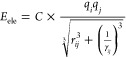170

171

172

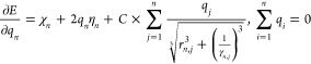173

Figure 75.

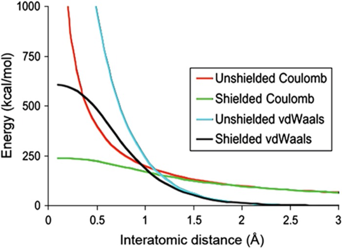
Plot of the Coulombic and VDW energies versus distance. A shielding term is applied to prevent these energies from becoming too large. Reprinted with permission from ref (168). Copyright 2011 Elsevier.

Figure 76.

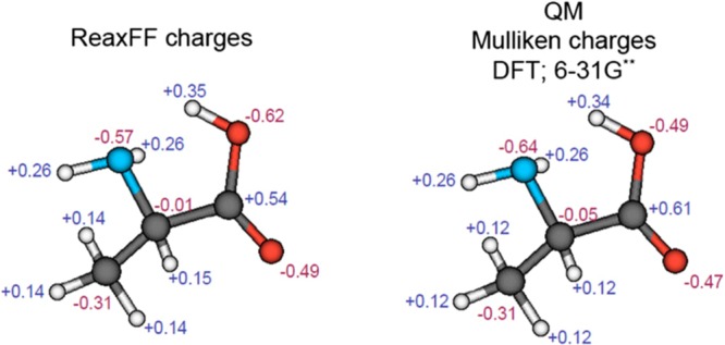
Comparison of the ReaxFF calculated charges versus QM values for the same molecule. The ReaxFF closely reproduces the Mullikan charges on each atom and models the polarizability of the molecule. Reprinted with permission from ref (168). Copyright 2011 Elsevier.

The ReaxFF force field is parametrized using the APM (see section 4.2.5) with the fitting being done against a variety of target properties from QM calculations. Different weights can be assigned to different data types during the parameter optimization process. Some recent works have been introduced to facilitate the parameter optimization of ReaxFF.^995−998 ReaxFF is not only able to simulate stable molecules but also relevant resonance structures, radical species, and reaction processes. ReaxFF is considerably faster than QM methods and can perform with good accuracy in carefully parametrized cases. For instance, the hydrocarbon reaction force field (ReaxFF^CH) offers an accuracy similar to that of the PM3 method, and is generally 100 times faster than PM3, which is itself ∼100 times faster than ab initio QM calculations.⁹⁸⁷

6.5.2. Examples

ReaxFFs have been developed for various metal-containing systems such as magnesium hydrides,⁹⁹⁹ lithium-containing complexes,¹⁰⁰⁰ TM-catalyzed reactions,⁹⁹⁴ platinum surfaces,¹⁰⁰¹ gold,⁹⁹³ vanadium oxide catalysts,¹⁰⁰² zinc oxide,¹⁰⁰³ cobalt nanoparticles,¹⁰⁰⁴ etc. ReaxFF-based models have also been applied to biological systems including DNA¹⁰⁰⁵ and proteins.¹⁰⁰⁶ Three examples of ReaxFFs about modeling the TM related systems are summarized below.

Chenoweth et al. parametrized ReaxFF for the reactions of hydrocarbons catalyzed by vanadium oxide solids.¹⁰⁰² 700 QM optimized structures and calculated energies were used to parametrize the reactive potential. These data points were related to bond dissociation processes, angle and dihedral distortions, energy changes of model reactions, bulk data on vanadium metals (BCC, FCC, A15, simple cubic, and diamond), and bulk data on vanadium oxides at different oxidation states. A MD simulation was carried out on a system consisting of a V₂O₅ slab (001) surface (containing 504 atoms), and 30 methanol molecules with a 0.25 fs time-step was used in the simulation. 250 ps of simulation was performed using a dual temperature thermostat algorithm (650 K for the slab to prevent it from melting and 2000 K for the methanol molecules). The resultant product distribution is shown in Figure 77. The simulation revealed CH₃OH molecules being converted to CH₂O molecules via two separate hydrogen absorption reactions by two surface V=O groups (with the CH₂OH radical as an intermediate species). Additional energy path scans indicated that the C–H dissociation path was preferred over O–H dissociation on the fully oxidized slab. Furthermore, water formation was observed during the simulation. Consistent with temperature-programmed desorption (TPD) experiments, the simulation results also supported interlayer bonding stabilization that facilitates water desorption at the vanadium oxide surface.

Figure 77.

Product distribution observed during the NVT-MD simulation of CH₃OH exposed to V₂O₅ (001) using ReaxFF. Only major products are shown explicitly; minor intermediates are included as “others”, and carbon-containing intermediates bound to the V₂O₅ surface are included as “surface carbon species”. Reprinted with permission from ref (1002). Copyright 2008 American Chemical Society.

Nielson et al. investigated the branching process of carbon fragments catalyzed by metal atoms using a ReaxFF model.⁹⁹⁴ An E_C2 term was added to the hydrogen carbon ReaxFF (ReaxFF^CH) to destabilize the C₂ radical. This is because the C–C bond in C₂ radical is weaker than a double bond, while ReaxFF^CH makes this bond even stronger than a triple bond. A number of QM calculated structures and energies were used in the parametrization process. These data points were related to the ground and intermediate states of species relevant to the system being studied. A MD simulation was carried out with 0.1 fs time-step at 1500 K under the NVT ensemble. Five monocyclic C₂₀ and 10 acyclic C₄ fragments were modeled in the system. No branching reactions were observed after 90 ps of simulation. Another three simulations were performed with each having 15 metal atoms added into the system (with 15 Co, Ni, and Cu atoms, respectively). To prevent metal clustering and facilitate metal carbon linkage, bond energies between the metal atoms were set to zero. As shown in Figure 78, considerable branching happens in the systems containing Co or Ni atoms, while the system containing Cu atoms showed less branching. This is consistent with experimental results. Figure 79 shows the structure of the system containing 15 Ni atoms after 750 ps of simulation, in which nanotude-like species were observed.

Figure 78.

Configurations obtained after 90 ps of NVT-MD simulation using ReaxFF without metal (a) and with 15 Co (b), Ni (c), and Cu (d). Reprinted with permission from ref (994). Copyright 2005 American Chemical Society.

Figure 79.

Configuration obtained from the NVT-MD simulation using ReaxFF with 15 Ni atoms after 750 ps. Reprinted with permission from ref (994). Copyright 2005 American Chemical Society.

The CN of Cu²⁺ ion in aqueous solution has been the subject of some debate.¹⁰⁰⁷ The point of contention is whether the CN is equal to 5 or 6 in the first solvation shell of a Cu²⁺ ion. Moreover, the role of the Jahn–Teller effect is also an issue drawing attention. van Duin et al. parametrized ReaxFF for Cu/O/H mixed systems using a training set containing Cu_x(OH)_y(H₂O)_z^2–y clusters, Cu, CuO, and Cu₂O crystals, along with various Cu(H₂O)₅²⁺ and Cu(H₂O)₆²⁺ structures.¹⁰⁰⁸ 133 ps of MD simulation was performed for a system containing one Cu²⁺ ion and 216 water molecules in the NVT ensemble at 300 K. It was shown that the ReaxFF model reproduced the Jahn–Teller effect in the first solvation shell. The dual-peak characteristic is clearly seen in the Cu–O RDF (see Figure 80). The ReaxFF simulation gave a 1.94 Å distance for the central copper to its equatorial oxygen and a 2.27 Å distance for the central copper to its axial oxygen. This agreed with available experimental data obtained from EXAFS and LAXS (distances of 1.95 and 2.29 Å, respectively). Meanwhile, the Jahn–Teller inversion rate was determined to be ∼5 ps from the ReaxFF simulation, which is in good agreement with the value of 5.1 ± 0.1 ps estimated from a ¹⁷O NMR study. Additional simulations suggested that even with 6-coordination dominating, 5-coordinate structures do occasionally appear.

Figure 80.

Cu–O RDF and integral as obtained from a ReaxFF MD simulation on a [Cu(H₂O)₂₁₆]²⁺ system at T = 300 K. Reprinted with permission from ref (1008). Copyright 2010 American Chemical Society.

6.6. Advantages and Drawbacks: More Accurate but with More Parameters

It is reasonably well established that polarizable models afford better accuracy than unpolarized models, especially for metal-containing systems. One significant advantage of polarizable models is that they can accurately represent molecules in the gas, liquid, and interfacial phases due to their ability to respond to the surroundings. Unpolarized models, on the other hand, are typically designed for simulations in specific environments. However, the improvement of polarizable models over unpolarized ones is not always guaranteed and depends on parameter quality, which implies polarizable models still have room to improve. Because unpolarized models are usually designed for a single phase, only using them for simulations they were designed for can mitigate their disadvantages.

On the down side, polarizable models have more complicated parametrization schemes and usually require the determination of more parameters that add to their complexity. For polarizable models, the spectre of overfitting can rear its ugly head in complicated parametrization processes. Meanwhile, parameters in the polarizable models may afford limited transferability and reparametrization may be needed when applying to different systems. Furthermore, polarizable models also share some drawbacks with unpolarized models when modeling metal ions: for example, the balance of ion–water and ion–ion interactions in ionic solutions needs be considered to reproduce properties at high salt concentrations. Moreover, it is also hard to reproduce the Jahn–Teller effect using polarizable models (except for ReaxFF, which implicitly includes this effect). We have shown several examples in section 7.2 involving the incorporation of the AOM/VB approach into the AMOEBA force field and the LF model into the SIBFA approach. These examples all showed improvement in the representations of the Jahn–Teller effect.

7. Models Based on the Angular Overlap Model and Valence Bond Theory

The nonbonded and bonded models use atomic cores with charge and VDW interactions to represent each particle, while the polarizable models add the induction effect to the particle interactions. However, all of these models do not explicitly take the orbital effects into account and struggle to simulate the Jahn–Teller effect, which is related to the d-orbital splitting. The AOM,^1009,1010 a SE MO approach, and models based on the VB theory offer ways to effectively model the Jahn–Teller effect. These approaches are all based on the overlap between atomic/hybrid orbitals. Deeth and co-workers have developed and applied the LFMM approach,¹⁰¹¹ while Landis and co-workers have incorporated a Fourier angle term into the MM model to create the SHAPES force field.¹⁹⁷ The latter have also incorporated the VB theory into a force field (so-called the VALBOND model).^1012−1015 Xiang and Ponder have incorporated the AOM and VB approaches into the AMOEBA polarizable force field.^1016,1017 Piquemal et al. have merged the LFMM model into the SIBFA polarizable force field.¹⁰¹⁸ These methods can model the Jahn–Teller effect, and offer more sophisticated approaches for ongoing and future force field development for TM complexes. In general, the AOM model is more suitable to systems with strong ionic characteristics, while the VB-based models can simulate systems with strong covalent effects. This is because the hybrid orbitals in the VB theory are based on covalent bonding, whereas the AOM-based models are atomic orbital based, which is more suitable for compounds that are more ionic. However, these models generally do not incorporate the electrostatic and polarization potential explicitly, which reduces their accuracy to represent long-range behavior (e.g., electrostatic, polarization) of metal centers. Electrostatic parameters can be incorporated to better account for long-range interactions, and they have a limited influence on geometric predictions but have a strong influence on energetic properties.^1019,1020 In what follows, we briefly review the approaches summarized above.

7.1. Applied to Unpolarized Models

7.1.1. LFMM Model

Deeth and co-workers described the LFMM (initially called CLFSE) model to incorporate the ligand field stabilization energy (LFSE) into the molecular modeling of TMs. Burton et al. created the Cellular LFSE (CLFSE)/MM model and applied it to Ni²⁺- and Cu²⁺-containing molecules.¹⁰¹¹ Its formulation is given in eq 174. It uses a Morse potential to represent bond stretching, and a 9-6 LJ potential for the nonbonded interactions (only for the 1-3 ligand–ligand interactions and between atoms separated by more than three bonds). Metal-containing angle and torsion interactions were assigned zero values. Electrostatic interactions were not included in the model. The CLFSE term was included in the total energy and was calculated on the basis of eq 175. Herein, ϱ(d_i) is the occupation number (usually 0, 1, or 2), while ε(d_i) is the d-orbital energies, which is obtained by diagonalization of the 5 × 5 d-orbital matrix (eq 176, where V_LF is the ligand field potential between d-orbitals i and j). Different spin states can be modeled by simply changing the occupancies of the d-orbitals. In the CLFSE model, each M–L interaction is divided into separate σ and π (including πx and πy) components, which are characterized by the e_σ, e_πx, and e_πy energy parameters (count as different modes; see eq 176). The e_σ, e_πx, and e_πy parameters are represented by eq 177, where a_n,k,ML is the fitting parameter. The ligand field splitting energy (Δ_oct) is proportional to 1/r⁵, where r is the distance between the metal ion and its ligating atom. Because Δ_oct = 3e_σ for simple ligands with σ bonds to the metal ion (such as amines), e_σ should also be proportional to 1/r⁵. In their work, they only developed the e_σ parameter for Ni²⁺/Cu²⁺ bound by a nitrogen atom. The e_σ parameter was represented by a linear equation (see eq 178) with r as the distance between the metal ion and its ligating atom.

174

175

176

177

178

Results showed that CLFSE/MM model offered comparable or better results relative to conventional MM models. It effectively simulated the Jahn–Teller effect, and correctly reproduced geometries of Ni²⁺–N and Cu²⁺–N bonds regardless of the CNs, molecular geometries, and ligating ligand types used in their investigation.

The LFMM model can also be used to simulate Werner-type compounds (which are more ionic in character) that are affected by the Jahn–Teller effect (e.g., [CuCl₄]^2–)¹⁰²¹ and complexes that have important contributions from bonds involving s orbitals (e.g., WH₆).¹⁷⁸ Covalent organometallic compounds WMe₆ and WH₆ have a d⁰ electronic configuration but do not have octahedral geometries,¹⁷⁸ an effect that can be captured by VB-based method (summarized below) through inclusion of sdⁿ hybridization but can also be modeled by LFMM via inclusion of a stabilization energy term representing the contribution from the s orbitals.

Deeth et al. have implemented the LFMM model into the molecular operating environment (MOE) package in 2005, and, cleverly, called it DommiMOE (named after the Dommino program, which means “d-orbital in molecular mechanics for inorganics”).¹⁰²² Examples, combined with the MMFF94 force field, were shown in their work to validate the LFMM model. Results also showed that DFT calculations were useful in designing improved LFMM parameters.

Deeth has also applied the LFMM model to blue copper proteins.¹⁰²³ The AMBER ff94 force field was used to describe the organic ligands, while the Cu–S parameters for the LFMM model were fitted using DFT calculations. Results from cluster and protein calculations showed the good performance of the LFMM model (see Figures 81 and 82), allowing the authors to suggest that the LFMM method has “quantum-like” behavior and was ∼4 orders of magnitude faster than QM/MM calculations.

Figure 81.

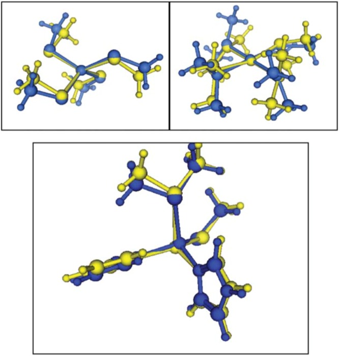
Overlay of LFMM (yellow) and DFT (blue) structures: top left, [Cu(SMe)₄]^2–, top right, [Cu(SMe₂)₄]²⁺, and bottom, the Type I active site model [Cu(im)₂(SMe)(SMe₂)]⁺. Reprinted with permission from ref (1023). Copyright 2006 Royal Society of Chemistry.

Figure 82.

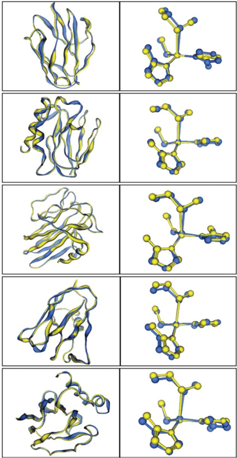
Overlay of XRD (yellow) and LFMM (blue) structures. Figures on the left show the superposition of the protein backbones, while those on the right show the optimal overlay of the trigonal [CuNNS] set. The proteins are given in the same order as Table 1 of ref (1023). Reprinted with permission from ref (1023). Copyright 2006 Royal Society of Chemistry.

Deeth et al. designed Fe²⁺ complexes that have spin crossover and light-induced excited spin state-trapped properties.¹⁰²⁴ They employed the LFMM model combined with MD simulations. The parameters were fit to DFT calculated data, and the LFMM-based MD simulations reproduced the low-spin and high-spin states for complexes with the FeN₆ motif (see Figures 83 and 84). The method uses much less time than DFT calculations, but in the end offered similar accuracy.

Figure 83.

Schematic diagrams of Fe²⁺ am(m)ine complexes. In the solid state, 1 and 2 are high-spin while 3 and 4 are low-spin. Reprinted with permission from ref (1024). Copyright 2010 American Chemical Society.

Figure 84.

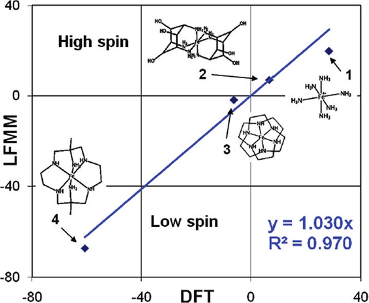
Comparison of theoretical spin-state energy differences (kJ/mol) for complexes 1–4. Reprinted with permission from ref (1024). Copyright 2010 American Chemical Society.

More recently, Foscato et al. implemented the LFMM into the Tinker MM package.¹⁰²⁵ It was shown that LFMM could deal with both the static calculations and the dynamic simulations.

7.1.2. SHAPES Force Field

Allured et al. described the SHAPES force field in 1991.¹⁹⁷ It uses a single Fourier term (see eq 179) instead of the harmonic equation to represent the angle bending interaction.

179

Similar to the Fourier term for a dihedral angle, n is the periodicity, φ is the phase, and k^F is the energy minimum. It was shown the Fourier term allowed energy changes both close to and far from typical equilibrium bond angles. Figure 85 shows the PES for the HOH angle obtained from HF calculations, a normal harmonic potential, and the Fourier angle potential. From this figure, we see that the Fourier angle potential better matches the results from QM-based methods than does the standard harmonic potential. The parameters for the Fourier angle potential can be calculated from parameters in a harmonic potential using the following equations:

180

181

182

Figure 85.

Comparison of PESs for angular distortion of water calculated by (●) the RHF method with a 6-31G* basis set, (○) a harmonic force field (k = 0.191 hartree/rad², θ_eq = 105.5°), and (■) a Fourier term (k^F = 0.0652 hartree, n = 2.42, φ = 74.50°). Reprinted with permission from ref (197). Copyright 1991 American Chemical Society.

Moreover, the Fourier representation is consistent with the AOM (see the appendix from their work).¹⁹⁷ The geometry representation in SHAPES is based on spherical internal coordinates. As in many standard force fields, the bond term in the SHAPES force field is harmonic, the torsion term uses Fourier expansions, and the 12-6 LJ equation was used to represent the VDW interactions. Electrostatic interactions were not considered in the parametrization process, which was based on normal coordinate analysis and PES scans based on QM calculations. It was shown that the so-derived force field reproduced the molecular structures of different square-planar Rh complexes to good accuracy (RMSDs of bond lengths ±0.02 Å and of angles ±3°). Tests including electrostatic interactions based on the QEq formulation from Rappe et al.⁸⁶⁸ demonstrated that inclusion of the electrostatic interactions had a trivial influence on structure prediction, implying that the derived parameters could be transferred to models including charge interactions. Using force constants based on normal coordinate analysis, they observed that the force constants inside ligands decreased when ligated to a metal ion. For example, k_b for the N–H bond decreases from 460 for a free ammonia to 410 kcal/mol·Å^–2 for a coordinated ammonia, along with the k_θ for the H–N–H angle decreases from 44 to 40 kcal/mol·rad^–2. However, in later work, Cleveland and Landis reported that the angular representation used in the SHAPES force field makes the bipyramidal geometry too rigid with respect to distortion to the square pyramidal geometry.¹⁰¹³

Doman et al. created force field models for linear metallocenes [M(Cp)₂] (where Cp = cyclopentadienyl) for a series of TMs, where almost all of the force constants were obtained on the basis of experimental data.¹⁰²⁰ Fourier terms were used for the angles that have the metal ion as their center atom, while harmonic terms were used for the other angles. To model these sandwich compounds, dummy atoms were placed in the centers of the five-member rings of the Cp groups and then bound to the central metal ion. A dihedral term was used to model the 1-5 interaction between the Cp carbon-dummy-metal-dummy-Cp carbon, which represents the rotation along the ligand metal axis (see Figure 86). The Columbic equation was used with a distance-dependent dielectric constant, and atomic charges were determined on the basis of the FQ method and updated every 50 steps in the energy minimization. It was shown that inclusion of electrostatic interactions caused limited impact on the molecular geometry but exerted considerable influence on the molecular energy. The derived force field reproduced the geometries of the metallocenes, even for those highly strained examples.

Figure 86.

Representation of the skeletal modes of a linear metallocene. The Cp rings are represented by horizontal lines and the metal by a dark circle. The 1,5-dihedral angle, α, the M–D stretch, a, the D–M–D, β, and the C–D–M bend, γ, are shown. Reprinted with permission from ref (1020). Copyright 1992 American Chemical Society.

7.1.3. Valence Bond-Based Models

Root et al. have developed the so-called VALBOND force field using concepts from the VB theory.¹⁰¹² They note that the conceptual foundation of MM aligns better with the localized bonds between hybrid orbitals (a perspective of VB theory) than it does with the delocalized LCAO picture from MO theory. The VALBOND model has an angular term based on the hybrid orbital strength function (see eqs 183–186). In these equations, α and Δ are the angle and overlap integral between two sp^mdⁿ hybrid orbitals, respectively. Functions of generalized strength S(α) and maximum possible strength S^max are shown in eqs 184 and 185, respectively. The final energy is determined on the basis of the pair defect approximation (PDA, see eq 183) where k is a scaling parameter.

183

184

185

186

Using sp³ hybrid orbitals as an example, the value of S^max = 2 is obtained using eq 185, and is derived using eq 186. When α = 109.5°, Δ = 0.0, which means the two orbitals are orthogonal, and S(α) equals S^max, yielding an E_angle (see eq 183) value of zero. The strength functions for sp³, sp², sp¹, and pure p orbitals are shown in Figure 87.

Figure 87.

Strength functions for sp³, sp², sp¹, and pure p orbitals. Reprinted with permission from ref (1012). Copyright 1993 American Chemical Society.

The only parameters that need to be determined in this formulation are the scaling parameter k and the hybridization of each bond orbital. They used simple Lewis structures and a quantitative representation of Bent’s rule to determine the hybridization of an individual bond. In the VALBOND representation, there are weighting factors for each combination of elements, and these weighting factors were determined on the basis of several rules. Rather than delineate them, herein we refer the reader to the original literature for full details.¹⁰¹² The scaling parameters were determined such that experimental vibration frequencies were accurately reproduced, and via this process it was shown that the scaling parameters did not significantly vary. A value of ∼163 kcal/mol for bonds containing hydrogen atoms and ∼220 kcal/mol for the other bonds afforded a good estimation. Overall, it was shown that the VALBOND force field reproduced molecular geometries and vibrational frequencies to good accuracy with a small number of parameters.

The VB model can handle situations involving delocalized bonding arrangements, like that seen in 3-center-4-electron (3c4e) bonds, which are observed in hypervalent (HV) molecules. Modeling HV molecules is a challenge for traditional MM models. Cleveland and Landis extended the VALBOND force field to handle HV compounds involving p-block elements.¹⁰¹³ Through the incorporation of resonance structures representing 3c4e bonds into VALBOND, these authors showed that it was possible to model HV molecules. To accomplish this, they added eq 187 to the VALBOND formulation to represent the 3c4e bond. In this equation, BOF stands for the bond order factor, and α and Δ are the bond angle and overlap integral between two interacting orbitals (e.g., for the F–Xe–F molecule, the two orbitals are the σ* hybrid orbital of [Xe–F]⁺ and the lone pair of F^–, respectively). This strength function favors the linear configuration: when α = 180°, α + π = 360°, making the overlap integral Δ = 0, yielding a minimum value for E(α). k_α is a scaling parameter and was set to 260 kcal/mol in their work. The bond, dihedral, improper torsion, and VDW terms were all taken from the CHARMM force field.

187

To model more complicated systems, such as ClF₃, which has both 2-center-3-electron (2c3e) and 3c4e bonds, different resonance configurations need to be considered. As shown in eqs 188 and 189, the total angle bending energy is represented by a mixture of energies of different resonance structures. Herein, c_n means the mixing coefficients, which are geometry dependent and determined on the basis of the HV angles inside each resonance configuration (see eq 189).

188

189

An offset term was added for the nonhomoleptic HV molecules, and it is related to the electronegativities of the ligands in the 3c4e bond (see eqs 190 and 191).

190

191

Herein, a and b represent two different atoms in the HV angle j of the ith MM configuration. en_lig and en_c.a. are the electronegativities of the ligand and the central atom, respectively, while ss is a scaling factor. ss is 1 when the electronegativity difference is positive and is 2 when the difference is negative. This offset representation gives a lower energy when the electronegativity of the ligand is larger than the central atom, and a higher energy in the converse. Results showed this HV-VB scheme reproduced the PESs, geometries, vibrational frequencies, site-preference, and fluxional pathways and was able to manifest ligand site exchange processes.

Landis et al. extended the VALBOND force field to metal alkyls and hydrides.¹⁰¹⁴ They used the 12-electron rule (based on sdⁿ hybridization) instead of the 18-electron rule to determine the hyper-valency of the TM complexes. This model can represent different configurations (such as square-planar, trigonal planar, octahedral) of TM complexes. It uses eq 192 to determine the mixing coefficients. This is because, while eq 189 is good for modeling spⁿ hybridized orbitals, it is less suitable for orbitals with more than 67% d-character. The scaling factors (k, in eq 183) for some TMs were parametrized on the basis of QM calculated frequencies for their hydrides. On the basis of these values, the scaling factors for the other TMs investigated were determined through interpolation/extrapolation.

192

Finally, it was shown that VALBOND reproduced the angles of 36 TM complexes with an average RMSD of less than 5°.

Firman and Landis extended VALBOND to TM complexes involving π-bonds.¹⁰¹⁵ When modeling π bonds in TM complexes, the VALBOND formulation becomes more complicated due to the incorporation σ–π and π–π bond pairs. Equation 193 calculates the torsion energy between a metal dπ orbital and a ligand dπ orbital (see Figure 88), where ϕ is the torsion angle of PI–M–L–PI, with M, L, and PI represent the metal, ligand, and π-pseudoatom, respectively, r_m is 1.67 (whose value was empirically derived) times the distance between the two central atoms, and bo2 is the bond order of the M–L bond, whose value is 2 or 3. e_tπ is set to 260 kcal/mol, which was also empirically derived.

193

Figure 88.

Scheme of π-bonding p–d atomic orbitals in the VALBOND model. Reprinted with permission from ref (1015). Copyright 2001 American Chemical Society.

To evaluate the bonds formed by the dπ orbital of a metal and a sdⁿ σ-hybrid orbital from a ligand, the equation given in Figure 89 is used. It is based on the consideration that a cloverleaf-shaped orbital can be represented by a linear combination of two d_z²-shape orbitals (see Figure 90).

Figure 89.

Overlap representation between a dπ orbital (left) and a σ bond with sdⁿ hybridization (right). Reprinted with permission from ref (1015). Copyright 2001 American Chemical Society.

Figure 90.

Representation of a cloverleaf shaped orbital by two d_z2 shaped orbitals. Reprinted with permission from ref (1015). Copyright 2001 American Chemical Society.

The dπ–dπ overlap between two cloverleaf shaped orbitals was determined using:

194

where the details for the α, β, χ, and δ terms can be found in the original article.¹⁰¹⁵ In their work, a slightly modified formulation of the VALBOND force field was used. The new formulation gave the same results for homoleptic complexes and offered advantages when modeling nonhomoleptic complexes. Results reported by these authors show that the VALBOND force field can predict molecular structures for a number of TM complexes with metal–ligand multiple bonds.

To model situations where there is a trans influence, Tubert-Brohman et al. created the VALBOND-TRANS force field for octahedral complexes containing Ru, Os, Rh, and Ir.¹⁰²⁶ The trans influence (that is different from the trans effect, which is related to the substitution reaction rate¹⁰²⁷) is a phenomenon affecting the electronic ground state of a complex where a ligand has the tendency to weaken the bond trans to it.¹⁰²⁸ It causes bond lengthening and can affect the relative stabilities of different diastereomers. It can be explained by a 3c4e bond formed between the metal ion and its ligands in which a “stronger” ligand prefers to bond in a trans orientation to a weaker ligand. They proposed eq 195 to model the energy changes due to the trans influence, which is based on the consideration that the trans influence is maximized at 180°.

195

196

Herein, p_AB is an adjustable parameter, which is related to the metal and ligand types. The harmonic equation was used for the bond stretching term, while the equilibrium bond distance was determined from eq 196, which represents bond length changes associated with the trans influence. Herein, i_B and s_A indicate the “trans influence intensity” and “lengthening sensitivity”, respectively. The authors obtained parameters in eqs 195 and 196 for octahedral complexes containing Ru, Os, Rh, or Ir based on DFT calculated isomeric energies and optimized structures. Test calculations were carried out on two larger octahedral Ir complexes, and the obtained results showed that the VALBOND-TRANS force field was able to reproduce the DFT calculated isomeric energies and geometries, outperforming the VALBOND force field for the cases studied.

Recently, Jin et al. studied Cu oxidation/reduction in water and protein systems through MD simulations using the DFTB3/MM and VALBOND methods.¹⁰²⁹ DFTB3 is a SE QM method, which is able to study chemical reactions, while the VALBOND method is a fast MM method that can study structural properties but needs parametrization for specific oxidation states and coordination environments of the Cu ion. Both methods covered the nanosecond time scale during the MD simulations, and are more efficient than the QM/MM MD simulations based on ab initio or DFT methods. They found that DFTB3/MM and VALBOND all capture the coexistence of the five- and six-coordinated structures of Cu²⁺ in water, which is consistent with experiment. However, subtle differences exist between different approaches: the hybrid-DFT/MM, DFTB3/MM, and VALBOND methods favor a six-coordinated Cu²⁺ ion in water, as compared to that the five-coordinated structure is favored by the nonhybrid BLYP functional and experiment. MD simulations based on DFTB3/MM, the BLYP functional, and HSE functional support a two-coordinated Cu⁺ in water, while B3LYP/MM predicts a four-coordinated Cu⁺ ion. They proposed that these subtle properties are worth further investigation by experiment and computation. These authors also showed that the DFTB3/MM and VALBOND methods performed well in simulating the [Cu(NH₃)₄]⁺ and [Cu(NH₃)₄]²⁺ complexes in aqueous solution. Furthermore, the DFTB3/MM method well simulated the active site of plastocyanin (where the Cu ion is coordinated to two His, one Cys, and one Met residue), and its predicted reduction potential and reorganization energy agreed with experiment. Meanwhile, the authors proposed that improved description of the charged species in DFTB3 was important for better modeling the Cu⁺ ion in DFTB3/MM simulations.

7.2. Applied to Polarizable Models

7.2.1. SIBFA-LF Model

Piquemal et al. incorporated the ligand field (LF) effect based on the AOM model into SIBFA in 2003.¹⁰¹⁸ The SIBFA-LF model was parametrized to model systems containing Cu²⁺–O and Cu²⁺–N bonds. It was found that the SIBFA-LF approach reproduced the Jahn–Teller effect, giving an improved geometric prediction when compared to the SIBFA approach. For example, the SIBFA-LF method predicts the elongated octahedral geometry of the Cu²⁺–(H₂O)₆ complex with the axial and equatorial Cu–O distances at 2.17 and 1.99 Å, respectively. In comparison, SIBFA predicts the Cu²⁺–(H₂O)₆ complex as octahedral with the six Cu–O distances all equal to 2.06 Å. As shown in Figure 91, the SIBFA model predicts that the inner four water molecules in Cu²⁺(H₂O)₄(H₂O)₂ are tetrahedrally coordinated, while SIBFA-LF predicts them to be planar. The SIBFA-LF correctly predicts the quasi-planar D2d geometry for Cu²⁺ coordinated with four NH₃ groups, or four imidazole (ImH) groups (see Figure 92 for the latter case), while SIBFA predicts a tetrahedral geometry.

Figure 91.

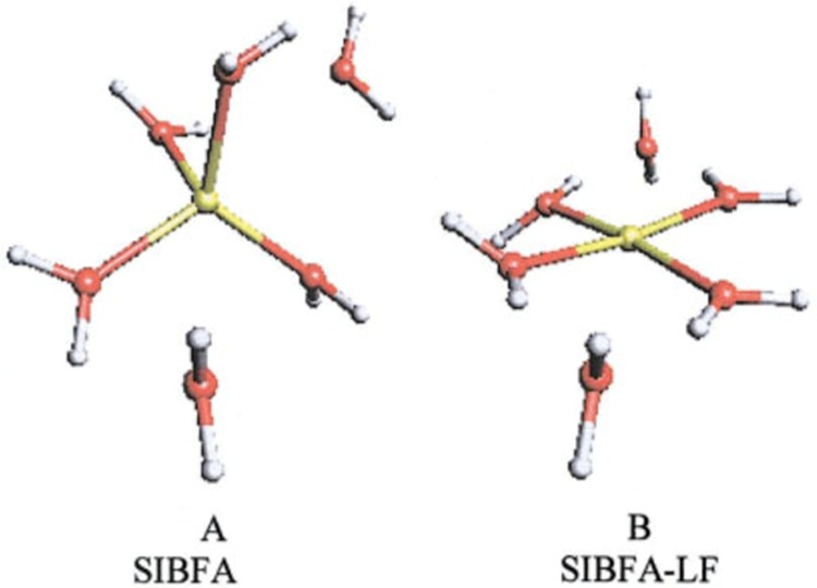
Minimized structure of Cu²⁺(H₂O)₄(H₂O)₂ based on the SIBFA (panel A) and SIBFA-LF (panel B) models. Reprinted with permission from ref (1018). Copyright 2003 John Wiley and Sons.

Figure 92.

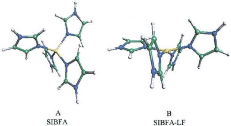
Minimized structure of Cu²⁺(ImH)₄ based on the SIBFA (panel A) and SIBFA-LF (panel B) models. Reprinted with permission from ref (1018). Copyright 2003 John Wiley and Sons.

7.2.2. AMOEBA-VB and AMOEBA-AOM Models

Xiang and Ponder incorporated the VB model into the AMOEBA force field for the Zn²⁺ and Cu²⁺ ions in aqueous solution.¹⁰¹⁷ The following representation was used:

197

198

where the U_resonance term represents the 3c4e bond, and the resonance structure number is equal to the number of O–M–O angles in the M²⁺(H2O)₆ complex. Here, W_k is the weighting factor for different resonance structures and is calculated on the basis of an empirical function. The U_VB-angle term is represented by the hybridization of the s, p, and d orbitals. The authors used an admixture of 10% s and 90% d to represent the bond formation between Cu²⁺ and its surrounding water molecules, while for Zn²⁺ 100% s orbital character was used. As shown in Figure 93, the VB angular potential for Cu²⁺ gives two energy minima at 90° and 180°, which agreed with a previous AOM model from Carlsson.¹⁰³⁰ The parameters were fit on the basis of QM calculations on M(H₂O)₄²⁺ and M(H₂O)₆²⁺ systems. Addition of the Jahn–Teller stabilization energy function from Comba and Zimmer¹⁰³¹ (see eqs 199 and 200, which are first-order harmonic equations, where r, r₀, Δ are the metal-ligand distance, average bonding distance, and a scaling parameter, respectively, with E_JT^xy applied to the in-plane ligands, and E_JT applied to the axial ligands) further improved the AMOEBA-VB model. However, this representation did not offer smooth transitions for axial–equatorial ligand interchange or coordination number changing, and therefore was not used in the subsequent MD simulation. Even with these modifications, the AMOEBA-VB model does not reproduce the dual peak in the first solvation shell of the Cu²⁺ ion during the aqueous phase MD simulation, and does not reproduce the two different bond lengths (elongation of the axial bond lengths) of the Cu(H₂O)₆²⁺ complex, but AMOEBA-VB predicts the square planar structure of the Cu(H₂O)₄²⁺ complex to be more stable than the tetrahedral one, offering an improved description over the AMOEBA model (see Figure 94). Meanwhile, their work showed that AMOEBA-VB gave results similar to those of the AMOEBA model for systems containing Zn²⁺.

199

200

Figure 93.

Schematic plot of VB angular potential for each 3c4e bond based on 10% s and 90% d hybridization. Reprinted with permission from ref (1017). Copyright 2012 John Wiley and Sons.

Figure 94.

Energy difference between square-planar (sq) and tetrahedral (te) tetra-aqua TM complexes; energy calculated by (U_sq – U_sq/empty) – (U_te – U_te/empty); data points from AMOEBA and AMOEBA-VB methods for [Zn(H₂O)₄]²⁺ overlap each other, as the differences in results are very small; see Tables 3 and 4 in the Supporting Information of ref (1017) for numerical values. U_sq/empty means system energy without considering the central ion. Reprinted with permission from ref (1017). Copyright 2012 John Wiley and Sons.

These authors have also incorporated the ligand field effect using the AOM for the Cu²⁺ ion in the AMOEBA force field.¹⁰¹⁶ In their work, they used MP2 calculated results as their benchmark data, because the DFT functionals, B3LYP and B2PLYP-D, gave divergent results. Similar to the AMOEBA-VB model described above, the AMOEBA-AOM model also effectively simulated the square-planar structure of the Cu(H₂O)₄²⁺ complex, giving it a lower energy than the tetrahedral one, while standard AMOEBA could not reproduce this effect (see Figure 95). The Jahn–Teller effect was well reproduced using this model in the gas phase for the Cu(H₂O)₆²⁺ complex, but in the aqueous phase this was not apparent because the dual peak was not observed in the Cu–O RDF in aqueous solution. The AMOBEA-AOM model predicted that the mean residence time of the first solvation shell water molecules for Cu²⁺ was 0.6–1.8 ns at room temperature, which was in accord with available experimental data (∼5 ns). In general, the AMOEBA-AOM force field was shown to outperform AMOEBA, when compared to QM calculated results. However, it elongates the Cu²⁺–S distance between the metal ion and Met group and could not well reproduce the sulfur ligand binding energies. The authors also proposed that AMOEBA-AOM might not be suitable for simulating system with strong covalent interactions, while the AMOEBA-VB model would be more appropriate.

Figure 95.

Potential energy difference between square-planar and tetrahedral tetra-aqua Cu²⁺ complexes with the water–water interaction removed. Negative values indicate that the square-planar structure is lower in potential energy than the tetrahedral geometry. Reprinted with permission from ref (1016). Copyright 2014 American Chemical Society.

8. Conclusions and Perspectives

8.1. Conclusions

There are a broad range of options to model metal ion-containing systems. However, for the uninitiated, the range of choices can be truly bewildering. The best way to proceed depends on a number of factors coupled with what exactly someone is trying to accomplish. To address this issue, we attempt to simplify the structure of the extensive discussion present in this Review by summarizing our suggestions for modeling TM-containing systems using QM and MM models. These suggestions are only meant to help initiate a study on metal ion-containing systems, and the reader is urged to review the sections most appropriate to their choice of model to understand their strengths and weaknesses and range of applicability in more detail. It is easy to go astray when modeling metal ions (even for so-called “experts”), so caveat emptor!

8.1.1. Quantum Mechanical Methods

Generally, the main group metal elements and Zn (it is easy to model zinc complexes as normal organic molecules) are well represented using DFT and post-HF methods with large basis sets. However, it is really challenging to model TMs, especially the middle series, in the periodic table due to their various spin states. Overall, the HF method is not suggested to use to study TM-containing systems due to the use of a single-determinant and omission of correlation effects. Care should be taken when one uses semiempirical methods to study such systems due to their minimal basis set. Moreover, attention should also be paid when using post-HF methods (e.g., MP2, CCSD, and CCSD(T) methods) to model TM species again because of their use of a single-determinant. Multiple reference methods such as CASSCF offer significant improvement in describing multireference systems like many TM species but are not practical for the study of large systems due to their extraordinary computational needs. Meanwhile, the DMRG method is a promising approach to model TM-containing systems with strong multireference characteristics.

The ccCA composite approach is recommended to obtain reference energy properties (e.g., HOFs) for TM species. DFT methods with their high computational speed could be very good choices to computationally study TM-containing systems. However, a large number of DFT functionals are available, and attention should be paid to choosing the appropriate one. In general, for pure metal systems, the functionals that approach the noble gas limit are recommended, while for multireference systems nonhybrid functionals are the best choice. For TM complexes containing organic ligands, the hybrid functionals may offer some improvements. However, the hybrid functionals with more than 40% HF exchange energy are not recommended. In terms of basis set choices, the basis sets of the ligands play a larger role than the basis set of the metal ions. All electron basis sets are recommended for the ligands, while effective core potentials can be used on the TMs. This is because the effective core potential considers the relativistic effect (which can be large for heavy metal elements) to some extent at a reduced computational cost. However, we note that the optimal basis set is also dependent on the DFT functional choice.

8.1.2. Force Field Models

For ions that have strong ionic characteristics (e.g., Na⁺, K⁺, F^–, Cl^–, Mg²⁺, Ca²⁺), the electrostatic term dominates its interaction with surrounding ligands. A nonbonded approach including electrostatic and VDW interactions is recommended for these situations, while charge scaling may be needed to better reproduce structural and dynamic properties in high salt concentrations. There are several classifications for nonbonded models: (1) The widely used 12-6 nonbonded model offers generally excellent results for the alkali metal ions except Li⁺. This is because the partial charges on these ions are close to the formal charge (+1e), making a point charge model an appropriate representation. (2) The 12-6-4, CDAM, DO, IDM, and LFMM models are suggested for use for the remaining monovalent ions as well as with divalent ions. This is because the 12-6 nonbonded model fails to describe the non-negligible polarization and CT effects for these ions, making it hard to reproduce multiple properties simultaneously. Meanwhile, the models listed above, which incorporate the polarization and CT interactions to some extent, can offer significant improvements. (3) The 12-6-4 and IDM models are suggested for highly charged ions. A combined model can also be used if the metal ion is only coordinated by water molecules.

The VALBOND and bonded models are recommended for use with TM complexes with strong covalent character or those that contain strong ion-ligand binding interactions that are largely invariant with time (i.e., no exchange or CN change). For the bonded model, the Seminario method is preferred because of its ease of use and good accuracy. An automatic parametrization method can be used for a metal site of specific interest. However, because the 1-3 nonbonded interaction is usually not included in the bonded model, it can fail for systems in which there are only attractive 1-4 electrostatic interactions (e.g., two adjacent coordinated water molecules). Hence, a bonded model with additional 1-3 terms or a nonbonded model with restrained interactions can be utilized in these situations. If one wants to study ligand switching at a specific coordination site, a hybrid unpolarized model can be used. To model the Jahn–Teller effect, the CDAM, bonded, LFMM, and ReaxFF models can be used. If one wants to study chemical reactions around metal ion-containing reactive centers, the cluster QM, QM/MM, or ReaxFF approaches are viable choices. The FQ model is the best approach to rapidly determine atomic charges and for screening large databases for ligand/material design. We have listed the availability of various models in several popular MD simulation packages in Table 5, and several parametrization tools for building up the bonded model are summarized in Table 6.

Table 5. Availability of Various Models in Several Popular MD Simulation Packages^a.

	model/software package
	AMBER1032	CHARMM1033	GROMACS1034	OpenMM1035	TINKER1036	Material Studio1037	LAMMPS1038
unpolarizeda	yes	yes	yes	yes	yes	yes	yes
FQ	no	yes	no	no	no	no	yes
DO	no	yes	yes	yes1039	no	no	yes
IDP	yes	yes	no	yes	yes	no	no
ReaxFF	no	no	no	no	no	yes	yes
LFMM	no	no	no	no	yes1025	no	no
VALBOND	no	yes1029	no	no	no	no	no

^aThe unpolarized models consist of the bonded, nonbonded, cationic dummy atom, combined, and coarse-grained models. All of these models have similar functional forms, and most MD simulation packages can handle all of them.

Table 6. Availability of Some Parametrization Tools To Facilitate Building Bonded Models of Metal-Containing Systems.

	language	method	support software	ref
Hess2FFa	Perl	Seminario	Gaussian	(669)
MCPBb	C++	Seminario/Z-matrix	Gaussian	(1)
parafreqc	Python	Burger	Gaussian	(682)
MCPB.pyd	Python	Seminario/Z-marix	Gaussian/GAMESS-US	(671)
CartHess2FC.pye	Python	Seminario/Z-marix	Gaussian/GAMESS-US	(1040)
VFFDTf	C++	Seminario	Gaussian/GAMESS-US/ORCA/Q-Chem/MOPAC	(672)

^aCan be downloaded from http://www.theochem.kth.se/~lixin/course/Hess2FF.pl.

^bAvailable in AmberTools from AmberTools1.5 to AmberTools16.

^cAvailable at http://www.chemistry.mcmaster.ca/ayers/5_software/para_freqv_1.3.tgz.

^dAvailable in AmberTools15, AmberTools16, and GitHub: https://github.com/Amber-MD/pymsmt.

^eAvaliable in AmberTools16 and GitHub: https://github.com/Amber-MD/pymsmt.

^fAvaliable at Dropbox, https://www.dropbox.com/sh/hlefz8xy8o23q44/AADZGTBN-aJ07flZ-kM0s4U6a?dl=0, and Baidu Cloud, https://pan.baidu.com/share/home?uk=2642812499.

8.2. Perspectives

Overall, it is still challenging to accurately model metal ion-containing systems, especially those containing TMs. Experimental studies, development of novel models and algorithms, as well as software development and application studies are all important to further facilitate research in this area. First, theoretical research of metal containing systems is being held back by the dearth of experimental data. With more and higher quality experimental data, computational methods (both QM and MM) could be better parametrized. With extensive experimental information at hand, benchmark studies to better understand the pros and cons of existing models can be carried out guiding the development of next generation models. Second, it is important to develop new models that better encapsulate the physics of metal ion-containing systems at an affordable cost. For example, models that accurately represent the structural dynamics of metal centers and bond breaking/formation processes are needed to accurately model TM-containing systems. Third, advanced algorithms that bridge the gap between quantum and classical models are needed. Current algorithms could be refined or new algorithms could be proposed that better reproduce the quantum effects in classical models. For example, algorithms that could allow classical models to better reproduce quantum calculated Hessian matrixes (like the Seminario method versus the Z-matrix method) would be beneficial. Finally, software development also plays an important role in facilitating model development, allowing for the rapid prototyping of various models to examine their applicability to a given problem.

Glossary

Abbreviations

ABEEM

atom-bond electronegativity equalization method

AC

activity coefficient

AIREBO

adaptive intermolecular REBO

AM1

Austin model 1

AM1-BCC

AM1 with bond charge correction

AMBER

assisted model building with energy refinement

AMOEBA

atomic multipole optimized energetics for biomolecular simulation

AOM

angular overlap model

BAR

Bennett acceptance ratio

BCC

body-centered cubic

BDE

bond dissociation energy

BOF

bond order factor

CASSCF

complete active space consistent field

CBAC

connectivity-based atom contribution

CBS

complete basis set

CC

coupled cluster

CCSD

coupled cluster with single and double excitations

CCSD(T)

coupled cluster with single, double, and perturbative triple excitations

CDAM

cationic dummy atom model

CFF

consistent force field

CG

coarse-grained

CHARMM

Chemistry at Harvard macromolecular mechanics

CHELP

charges from electrostatic potentials

CI

configuration interaction

CID

configuration interaction in the space of double substitutions

CLFSE

cellular LFSE

CMO

canonical molecular orbital

CN

coordination number

CNDO

complete neglect of differential overlap

CNS

crystallography and NMR system

COMB

charge-optimized-many-body

COMPASS

condensed-phase optimized molecular potentials for atomistic simulation studies

CPA

carboxypeptidase A

CPE

chemical potential equilibration

CPMD

Car–Parrinello molecular dynamics

CPU

central processing unit

CS

charge scaling

CSOV

constrained space orbital variation

CT

charge transfer

CTPOL

charge-transfer polarizable

CVFF

consistent valence force field

DC

diffusion coefficient

DDAP

density-derived atomic point

DDEC

density-derived electrostatic and chemical

DFT

density functional theory

DFTB

density functional tight binding

DMA

distributed multipole analysis

DMD

discrete molecular dynamics

DMRG

density matrix renormalization group

DNA

deoxyribonucleic acid

DO

Drude oscillator

DR

Drude rod

DREIDING

a generic force field developed by Mayo et al.

EA

electron affinity

EAM

embedded atom model

ECP

effective core potential

EDA

energy decomposition analysis

EEM

electronegativity equalization method

EPM

electrostatic potential map

EQeq

extended charge equilibration

ESP

electrostatic potential

EVB

empirical valence bond

EXAFS

extended X-ray absorption fine structure

FCC

face centered cubic

FEP

free-energy perturbation

FQ

fluctuating charge

FQ-DCT

FQ discrete charge-transfer

FS

Finnis–Sinclair

G1

Gaussian-1

G2

Gaussian-2

G3

Gaussian-3

G4

Gaussian-4

GAFF

general AMBER force field

GAM

gradient approximation for molecules

GEM

Gaussian electrostatic model

GGA

generalized gradient approximation

GME

Gmelinite

GPU

graphic processing unit

GROMOS

a force field associated with Groningen Machine for Chemical Simulations (GROMACS) software package

GSK3β

glycogen synthase kinase 3β

GolP

gold-protein

HCAI

human carbonic anhydrase I

HCAII

human carbonic anhydrase II

HCP

hexagonal close packed

HF

Hartree–Fock

HFE

hydration free energy

HO

hybrid orbital

HOF

heat of formation

HSAB

hard soft acid base

HV

hypervalent

Hp

Helicobacter pylori

IDM

induced dipole model

INDO

intermediate neglect of differential overlap

IOD

ion–oxygen distance of first solvation shell

IRF

interaction round a face

IP

ionization potential

IR

infrared

KA

Klebsella aerogenes

KBI

Kirkwood–Buff integral

LAXS

large-angle X-ray scattering

LB

Lorentz–Berthelot

LC

crystal lattice constant

LCAO

linear combination of atomic orbitals

LDA

local density approximation

LE

crystal lattice energy

LF

ligand field

LFMM

ligand field molecular mechanics

LFSE

ligand field stabilization energy

LIE

linear interaction energy

LJ

Lennard-Jones

LSDA

local spin density approximation

MAD

mean absolute deviation

MAPE

mean absolute percentage error

MARTINI

a coarse-grained force field developed by Marrink et al. for biomolecular simulations

MB-nrg

many-body-energy

MC

Monte Carlo

MCPB

metal center parameter builder

MD

molecular dynamics

MDEC

molecular dynamics electronic continuum

MIL

Material from Institute Lavoisier

MINDO

modified intermediate neglect differential overlap

MM

molecular mechanics

MM/GBSA

molecular mechanics generalized Born surface area

MM/PBSA

molecular mechanics Poisson–Boltzmann surface area

MMFF

Merck molecular force field

MMP

matrix metalloproteinase

MNDO

modified neglect of diatomic overlap

MO

molecular orbital

MOE

molecular operating environment

MOF

metal–organic framework

MOLPRO

a quantum chemistry software package developed by Knowles, Werner, and co-workers

MP2

Møller–Plesset perturbation theory to the second order

MP3

Møller–Plesset perturbation theory to the third order

MP4

Møller–Plesset perturbation theory to the fourth order

MS-EVB

multistate empirical valence bond

MSINDO

modified SINDO

NMR

nuclear magnetic resonance

NNLC

nearest neighbor ligands correction

NPA

natural population analysis

OPC

optimal point charge

OPLS

optimized potentials for liquid simulations

OPLS-AA

OPLS with all atom representation

OPLS-AAP

OPLS-AA with induced dipoles

OPLS-CM1AP

OPLS with with CM1A charge and induced dipoles

ORCA

a quantum chemistry software package developed by Neese and co-workers

PBC

periodic boundary condition

PBF

Poisson–Boltzmann finite element continuum solvation model

PCFF

polymer consistent force field

PCM

polarizable continuum model

PDA

pair defect approximation

PDB

protein databank

PEOE

partial equalization of orbital electronegativity

PES

potential energy surface

PFF

polarizable force field

PHF

partial Hessian fitting

PIPF

polarizable intermolecular potential function

PM3

parametric method 3

PME

particle mesh Ewald

PMF

potential of mean force

POL

polarization

PQEq

periodic charge equilibration

Q-Chem

a quantum chemistry software package developed by Q-Chem Inc.

QCISD

quadratic configuration interaction singles doubles

QEq

charge equilibration

QM

quantum mechanics

QM/MM

quantum mechanics/molecular mechanics

QPCT

quantum calibrated polarizable-charge transfer

QSAR

quantitative structure-acitivity relationship

RASSCF

restricted active space consistent field

RDF

radial distribution function

REBO

reactive empirical bond order

REPEAT

repeating electrostatic potential extracted atomic

RESP

restrained electrostatic potential

RG

renormalization group

RHF

restricted Hartree–Fock

RMS

root mean square

RMSD

root mean square deviation

RMSF

root mean square fluctation

RNA

ribonucleic acid

ROHF

restricted-open-shell-Hartree–Fock

RVS

reduced variational space

ReaxFF

reactive force field

SAPT

symmetry-adapted perturbation theory

SC

Sutton–Chen

SCC-DFTB

self-consistent charge density functional tight binding

SCF

self-consistent field

SCS

spin component scaled

SE

semiempirical

SFC

semifluctuating charge

SHAPES

a classical force field developed by Landis et al.

SIBFA

sum of interactions between fragments computed ab initio

SINDO

symmetrically orthogonalized INDO

SINDO1

a semiempirical quantum mechanics method developed by Jug et al.

SLEF

short–long effective function

SNase

staphylococcal nuclease

SOD

sodalite

SPC

simple point charge water model

SPC/E

extended simple point charge water model

SWM4-DP

simple water model with four sites and Drude polarizability

SWM4-NDP

simple water model with four sites and negative Drude polarizability

TB

tight-binding

TB-SMA

tight-binding with second moment approximation

TI

thermodynamic integration

TIP3P

transferable intermolecular potential 3-point charges

TIP4P

transferable intermolecular potential 4-point charges

TIP4P_EW

TIP4P water model for Ewald summation

TIPS

transferable intermolecular potential function

TM

transition metal

TPD

temperature-programmed desorption

TraPPE

transferable potentials for phase equilibria

TST

transition state theory

TTM

Thole-type model

UFF

Universal force field UNRES United residue

VALBOND

a force field developed by Landis et al. based on the VB theory

VB

valence bond

VDW

van der Waals

VESPR

valence shell electron pair repulsion

VFFDT

visual force field derivation toolkit

XRD

X-ray diffraction

ZAFF

zinc AMBER force field

ZIF

zeolitic imidazolate framework

ZINDO

Zerner INDO method

ccCA

correlation consistent composite approach

ccCA-TM

ccCA for transition metals

pyMSMT

python metal site modeling toolbox

rp-ccCA

relativistic pseudopotential ccCA

Biographies

Pengfei Li graduated from Xiamen University in China with a B.S. degree in Chemistry in 2011. During his undergraduate studies, he obtained training in quantum chemistry in the laboratory of Prof. Zexing Cao. In 2011, he enrolled in the Ph.D. program at the University of Florida and entered Prof. Kenneth M. Merz Jr.’s lab. In 2013 the Merz laboratory transferred to Michigan State University where he obtained his Ph.D. degree in Chemistry in the summer of 2016. His Ph.D. research concentrated on the development of models and software tools for metal ion modeling. Currently, he is a Postdoctoral Research Associate in Professor Sharon Hammes-Schiffer’s lab at the University of Illinois at Urbana–Champaign.

Kenneth M. Merz Jr. is the Joseph Zichis Chair in Chemistry and Director of the Institute for Cyber Enabled Research (iCER) at Michigan State University. His research interest lies in the development of theoretical and computational tools and their application to biological problems including structure and ligand-based drug design, mechanistic enzymology, and methodological verification and validation. He has received a number of honors including election as an ACS Fellow, the 2010 ACS Award for Computers in Chemical and Pharmaceutical Research, election as a fellow of the American Association for the Advancement of Science, and a John Simon Guggenheim Fellowship.

Author Present Address

^† Department of Chemistry, University of Illinois at Urbana-Champaign, Urbana, Illinois 61801, United States.

The authors declare no competing financial interest.

References

- Peters M. B.; Yang Y.; Wang B.; Füsti-Molnár L.; Weaver M. N.; Merz K. M. Jr Structural Survey of Zinc-Containing Proteins and Development of the Zinc Amber Force Field (Zaff). J. Chem. Theory Comput. 2010, 6, 2935–2947. 10.1021/ct1002626. [DOI] [PMC free article] [PubMed] [Google Scholar]
- Perez V.; Chang E. T. Sodium-to-Potassium Ratio and Blood Pressure, Hypertension, and Related Factors. Adv. Nutr. 2014, 5, 712–741. 10.3945/an.114.006783. [DOI] [PMC free article] [PubMed] [Google Scholar]
- Haddy F. J.; Vanhoutte P. M.; Feletou M. Role of Potassium in Regulating Blood Flow and Blood Pressure. Am. J. Physiol. Regul. Integr. Comp. Physiol. 2005, 290, R546–R552. 10.1152/ajpregu.00491.2005. [DOI] [PubMed] [Google Scholar]
- Altura B.; Altura B. Interactions of Mg and K on Blood Vessels--Aspects in View of Hypertension. Review of Present Status and New Findings. Magnesium 1983, 3, 175–194. [PubMed] [Google Scholar]
- Bukoski R. D. Dietary Ca2+ and Blood Pressure: Evidence That Ca2+-Sensing Receptor Activated, Sensory Nerve Dilator Activity Couples Changes in Interstitial Ca2+ with Vascular Tone. Nephrol. Dial. Transplant. 2001, 16, 218–221. 10.1093/ndt/16.2.218. [DOI] [PubMed] [Google Scholar]
- Page M. J.; Di Cera E. Role of Na+ and K+ in Enzyme Function. Physiol. Rev. 2006, 86, 1049–1092. 10.1152/physrev.00008.2006. [DOI] [PubMed] [Google Scholar]
- Aperia A.; Holtbäck U.; Syren M.; Svensson L.; Fryckstedt J.; Greengard P. Activation/Deactivation of Renal Na+, K (+)-Atpase: A Final Common Pathway for Regulation of Natriuresis. FASEB J. 1994, 8, 436–439. [DOI] [PubMed] [Google Scholar]
- Møller J.; Lind K.; Andersen J. Enzyme Kinetics and Substrate Stabilization of Detergent-Solubilized and Membraneous (Ca2+ + Mg2+)-Activated Atpase from Sarcoplasmic Reticulum. Effect of Protein-Protein Interactions. J. Biol. Chem. 1980, 255, 1912–1920. [PubMed] [Google Scholar]
- Lee S. H.; Johnson J. D.; Walsh M. P.; Van Lierop J. E.; SUTHERLAND C.; Ande X.; Snedden W. A.; Danuta K.-K.; Fromm H.; Narayanan N. Differential Regulation of Ca2+/Calmodulin-Dependent Enzymes by Plant Calmodulin Isoforms and Free Ca2+ Concentration. Biochem. J. 2000, 350, 299–306. 10.1042/bj3500299. [DOI] [PMC free article] [PubMed] [Google Scholar]
- Ahvazi B.; Boeshans K. M.; Idler W.; Baxa U.; Steinert P. M. Roles of Calcium Ions in the Activation and Activity of the Transglutaminase 3 Enzyme. J. Biol. Chem. 2003, 278, 23834–23841. 10.1074/jbc.M301162200. [DOI] [PubMed] [Google Scholar]
- Robinson R.Structure of Signaling Enzyme Reveals How Calcium Turns It On. PLoS Biol. 2010, 8. [DOI] [PMC free article] [PubMed] [Google Scholar]
- Beinert H.; Kennedy M. C.; Stout C. D. Aconitase as Iron–Sulfur Protein, Enzyme, and Iron-Regulatory Protein. Chem. Rev. 1996, 96, 2335–2374. 10.1021/cr950040z. [DOI] [PubMed] [Google Scholar]
- Stephens P. J.; Jollie D. R.; Warshel A. Protein Control of Redox Potentials of Iron–Sulfur Proteins. Chem. Rev. 1996, 96, 2491–2514. 10.1021/cr950045w. [DOI] [PubMed] [Google Scholar]
- Ferguson-Miller S.; Babcock G. T. Heme/Copper Terminal Oxidases. Chem. Rev. 1996, 96, 2889–2908. 10.1021/cr950051s. [DOI] [PubMed] [Google Scholar]
- Solomon E. I.; Sundaram U. M.; Machonkin T. E. Multicopper Oxidases and Oxygenases. Chem. Rev. 1996, 96, 2563–2606. 10.1021/cr950046o. [DOI] [PubMed] [Google Scholar]
- Jacoby M. How Computers Are Helping Chemists Discover Materials That Don’t yet Exist. Chem. Eng. News 2015, 93, 8–11. [Google Scholar]
- Schaller R. R. Moore’s Law: Past, Present and Future. IEEE Spectrum 1997, 34, 52–59. 10.1109/6.591665. [DOI] [Google Scholar]
- Jacoby M. Chemistry by the Numbers. Chem. Eng. News 2013, 91, 51–55. 10.1021/cen-09136-cover6. [DOI] [Google Scholar]
- Götz A. W.; Williamson M. J.; Xu D.; Poole D.; Le Grand S.; Walker R. C. Routine Microsecond Molecular Dynamics Simulations with Amber on Gpus. 1. Generalized Born. J. Chem. Theory Comput. 2012, 8, 1542–1555. 10.1021/ct200909j. [DOI] [PMC free article] [PubMed] [Google Scholar]
- Salomon-Ferrer R.; Götz A. W.; Poole D.; Le Grand S.; Walker R. C. Routine Microsecond Molecular Dynamics Simulations with Amber on Gpus. 2. Explicit Solvent Particle Mesh Ewald. J. Chem. Theory Comput. 2013, 9, 3878–3888. 10.1021/ct400314y. [DOI] [PubMed] [Google Scholar]
- Shaw D. E.; Maragakis P.; Lindorff-Larsen K.; Piana S.; Dror R. O.; Eastwood M. P.; Bank J. A.; Jumper J. M.; Salmon J. K.; Shan Y.; et al. Atomic-Level Characterization of the Structural Dynamics of Proteins. Science 2010, 330, 341–346. 10.1126/science.1187409. [DOI] [PubMed] [Google Scholar]
- Jorgensen W. L.; Ruiz-Caro J.; Tirado-Rives J.; Basavapathruni A.; Anderson K. S.; Hamilton A. D. Computer-Aided Design of Non-Nucleoside Inhibitors of Hiv-1 Reverse Transcriptase. Bioorg. Med. Chem. Lett. 2006, 16, 663–667. 10.1016/j.bmcl.2005.10.038. [DOI] [PubMed] [Google Scholar]
- Bollini M.; Domaoal R. A.; Thakur V. V.; Gallardo-Macias R.; Spasov K. A.; Anderson K. S.; Jorgensen W. L. Computationally-Guided Optimization of a Docking Hit to Yield Catechol Diethers as Potent Anti-Hiv Agents. J. Med. Chem. 2011, 54, 8582–8591. 10.1021/jm201134m. [DOI] [PMC free article] [PubMed] [Google Scholar]
- Dziedzic P.; Cisneros J. A.; Robertson M. J.; Hare A. A.; Danford N. E.; Baxter R. H.; Jorgensen W. L. Design, Synthesis, and Protein Crystallography of Biaryltriazoles as Potent Tautomerase Inhibitors of Macrophage Migration Inhibitory Factor. J. Am. Chem. Soc. 2015, 137, 2996–3003. 10.1021/ja512112j. [DOI] [PMC free article] [PubMed] [Google Scholar]
- Gray W. T.; Frey K. M.; Laskey S. B.; Mislak A. C.; Spasov K. A.; Lee W.-G.; Bollini M.; Siliciano R. F.; Jorgensen W. L.; Anderson K. S. Potent Inhibitors Active against Hiv Reverse Transcriptase with K101p, a Mutation Conferring Rilpivirine Resistance. ACS Med. Chem. Lett. 2015, 6, 1075–1079. 10.1021/acsmedchemlett.5b00254. [DOI] [PMC free article] [PubMed] [Google Scholar]
- Mak L.; Liggi S.; Tan L.; Kusonmano K.; M Rollinger J.; Koutsoukas A.; C Glen R.; Kirchmair J. Anti-Cancer Drug Development: Computational Strategies to Identify and Target Proteins Involved in Cancer Metabolism. Curr. Pharm. Des. 2013, 19, 532–577. 10.2174/138161213804581855. [DOI] [PubMed] [Google Scholar]
- Wood J. M.; Maibaum J.; Rahuel J.; Grutter M. G.; Cohen N. C.; Rasetti V.; Ruger H.; Goschke R.; Stutz S.; Fuhrer W.; et al. Structure-Based Design of Aliskiren, a Novel Orally Effective Renin Inhibitor. Biochem. Biophys. Res. Commun. 2003, 308, 698–705. 10.1016/S0006-291X(03)01451-7. [DOI] [PubMed] [Google Scholar]
- Cole J. M.; Low K. S.; Ozoe H.; Stathi P.; Kitamura C.; Kurata H.; Rudolf P.; Kawase T. Data Mining with Molecular Design Rules Identifies New Class of Dyes for Dye-Sensitised Solar Cells. Phys. Chem. Chem. Phys. 2014, 16, 26684–26690. 10.1039/C4CP02645D. [DOI] [PubMed] [Google Scholar]
- Studt F.; Sharafutdinov I.; Abild-Pedersen F.; Elkjær C. F.; Hummelshøj J. S.; Dahl S.; Chorkendorff I.; Nørskov J. K. Discovery of a Ni-Ga Catalyst for Carbon Dioxide Reduction to Methanol. Nat. Chem. 2014, 6, 320–324. 10.1038/nchem.1873. [DOI] [PubMed] [Google Scholar]
- Kibsgaard J.; Tsai C.; Chan K.; Benck J. D.; Nørskov J. K.; Abild-Pedersen F.; Jaramillo T. F. Designing an Improved Transition Metal Phosphide Catalyst for Hydrogen Evolution Using Experimental and Theoretical Trends. Energy Environ. Sci. 2015, 8, 3022–3029. 10.1039/C5EE02179K. [DOI] [Google Scholar]
- Shamp A.; Zurek E. Superconducting High-Pressure Phases Composed of Hydrogen and Iodine. J. Phys. Chem. Lett. 2015, 6, 4067–4072. 10.1021/acs.jpclett.5b01839. [DOI] [PubMed] [Google Scholar]
- Yan F.; Zhang X.; Yu Y. G.; Yu L.; Nagaraja A.; Mason T. O.; Zunger A. Design and Discovery of a Novel Half-Heusler Transparent Hole Conductor Made of All-Metallic Heavy Elements. Nat. Commun. 2015, 6, 7308. 10.1038/ncomms8308. [DOI] [PubMed] [Google Scholar]
- Zurek E.; Yao Y. Theoretical Predictions of Novel Superconducting Phases of Bage3 Stable at Atmospheric and High Pressures. Inorg. Chem. 2015, 54, 2875–2884. 10.1021/ic5030235. [DOI] [PubMed] [Google Scholar]
- Riedel S.; Kaupp M. The Highest Oxidation States of the Transition Metal Elements. Coord. Chem. Rev. 2009, 253, 606–624. 10.1016/j.ccr.2008.07.014. [DOI] [Google Scholar]
- Wang G.; Zhou M.; Goettel J. T.; Schrobilgen G. J.; Su J.; Li J.; Schlöder T.; Riedel S. Identification of an Iridium-Containing Compound with a Formal Oxidation State of Ix. Nature 2014, 514, 475–477. 10.1038/nature13795. [DOI] [PubMed] [Google Scholar]
- Yu H. S.; Truhlar D. G. Oxidation State 10 Exists. Angew. Chem., Int. Ed. 2016, 55, 9004. 10.1002/anie.201604670. [DOI] [PubMed] [Google Scholar]
- Megyes T.; Grosz T.; Radnai T.; Bakó I.; Pálinkás G. Solvation of Calcium Ion in Polar Solvents: An X-Ray Diffraction and Ab Initio Study. J. Phys. Chem. A 2004, 108, 7261–7271. 10.1021/jp048838m. [DOI] [Google Scholar]
- Cotton F.; Curtis N.; Harris C.; Johnson B.; Lippard S.; Mague J.; Robinson W.; Wood J. Mononuclear and Polynuclear Chemistry of Rhenium (Iii): Its Pronounced Homophilicity. Science 1964, 145, 1305–1307. 10.1126/science.145.3638.1305. [DOI] [PubMed] [Google Scholar]
- Gagliardi L.; Roos B. O. Quantum Chemical Calculations Show That the Uranium Molecule U2 Has a Quintuple Bond. Nature 2005, 433, 848–851. 10.1038/nature03249. [DOI] [PubMed] [Google Scholar]
- Nguyen T.; Sutton A. D.; Brynda M.; Fettinger J. C.; Long G. J.; Power P. P. Synthesis of a Stable Compound with Fivefold Bonding between Two Chromium (I) Centers. Science 2005, 310, 844–847. 10.1126/science.1116789. [DOI] [PubMed] [Google Scholar]
- Clark D.; Schrock R. Multiple Metal-Carbon Bonds. 12. Tungsten and Molybdenum Neopentylidyne and Some Tungsten Neopentylidene Complexes. J. Am. Chem. Soc. 1978, 100, 6774–6776. 10.1021/ja00489a049. [DOI] [Google Scholar]
- Churchill M. R.; Youngs W. J. Crystal Structure and Molecular Geometry of W (. Tplbond. Ccme3)(: Chcme3) (Ch2cme3) (Dmpe), a Mononuclear Tungsten (Vi) Complex with Metal-Alkylidyne, Metal-Alkylidene, and Metal-Alkyl Linkages. Inorg. Chem. 1979, 18, 2454–2458. 10.1021/ic50199a025. [DOI] [Google Scholar]
- Beaumier E. P.; Billow B. S.; Singh A. K.; Biros S. M.; Odom A. L. A Complex with Nitrogen Single, Double, and Triple Bonds to the Same Chromium Atom: Synthesis, Structure, and Reactivity. Chem. Sci. 2016, 7, 2532–2536. 10.1039/C5SC04608D. [DOI] [PMC free article] [PubMed] [Google Scholar]
- Chaboy J.; Muñoz-Páez A.; Merkling P. J.; Marcos E. S. The Hydration of Cu2+: Can the Jahn-Teller Effect Be Detected in Liquid Solution?. J. Chem. Phys. 2006, 124, 064509. 10.1063/1.2165189. [DOI] [PubMed] [Google Scholar]
- Lipscomb W. N.; Sträter N. Recent Advances in Zinc Enzymology. Chem. Rev. 1996, 96, 2375–2434. 10.1021/cr950042j. [DOI] [PubMed] [Google Scholar]
- Danopoulos A. A.; Wilkinson G.; Sweet T. K.; Hursthouse M. B. Tert-Butylimido Compounds of Manganese-(Vii),-(Vi),-(V) and-(Ii); Nitrido, Amido, Alkyl, Zinc and Aluminium Compounds. J. Chem. Soc., Dalton Trans. 1995, 205–216. 10.1039/dt9950000205. [DOI] [Google Scholar]
- Jiang W.; DeYonker N. J.; Determan J. J.; Wilson A. K. Toward Accurate Theoretical Thermochemistry of First Row Transition Metal Complexes. J. Phys. Chem. A 2012, 116, 870–885. 10.1021/jp205710e. [DOI] [PubMed] [Google Scholar]
- Grossfield A.; Ren P.; Ponder J. W. Ion Solvation Thermodynamics from Simulation with a Polarizable Force Field. J. Am. Chem. Soc. 2003, 125, 15671–15682. 10.1021/ja037005r. [DOI] [PubMed] [Google Scholar]
- Lamoureux G.; Roux B. Absolute Hydration Free Energy Scale for Alkali and Halide Ions Established from Simulations with a Polarizable Force Field. J. Phys. Chem. B 2006, 110, 3308–3322. 10.1021/jp056043p. [DOI] [PubMed] [Google Scholar]
- Norrby P. O.; Liljefors T. Automated Molecular Mechanics Parameterization with Simultaneous Utilization of Experimental and Quantum Mechanical Data. J. Comput. Chem. 1998, 19, 1146–1166. . [DOI] [Google Scholar]
- Allinger N. L.; Zhou X.; Bergsma J. Molecular Mechanics Parameters. J. Mol. Struct.: THEOCHEM 1994, 312, 69–83. 10.1016/S0166-1280(09)80008-0. [DOI] [Google Scholar]
- Holm R. H.; Solomon E. I. Preface: Bioinorganic Enzymology. Chem. Rev. 1996, 96, 2237–2238. 10.1021/cr9604144. [DOI] [PubMed] [Google Scholar]
- Averill B. A. Dissimilatory Nitrite and Nitric Oxide Reductases. Chem. Rev. 1996, 96, 2951–2964. 10.1021/cr950056p. [DOI] [PubMed] [Google Scholar]
- Burgess B. K.; Lowe D. J. Mechanism of Molybdenum Nitrogenase. Chem. Rev. 1996, 96, 2983–3012. 10.1021/cr950055x. [DOI] [PubMed] [Google Scholar]
- Dismukes G. C. Manganese Enzymes with Binuclear Active Sites. Chem. Rev. 1996, 96, 2909–2926. 10.1021/cr950053c. [DOI] [PubMed] [Google Scholar]
- Eady R. R. Structure-Function Relationships of Alternative Nitrogenases. Chem. Rev. 1996, 96, 3013–3030. 10.1021/cr950057h. [DOI] [PubMed] [Google Scholar]
- Flint D. H.; Allen R. M. Iron-Sulfur Proteins with Nonredox Functions. Chem. Rev. 1996, 96, 2315–2334. 10.1021/cr950041r. [DOI] [PubMed] [Google Scholar]
- Hille R. The Mononuclear Molybdenum Enzymes. Chem. Rev. 1996, 96, 2757–2816. 10.1021/cr950061t. [DOI] [PubMed] [Google Scholar]
- Holm R. H.; Kennepohl P.; Solomon E. I. Structural and Functional Aspects of Metal Sites in Biology. Chem. Rev. 1996, 96, 2239–2314. 10.1021/cr9500390. [DOI] [PubMed] [Google Scholar]
- Howard J. B.; Rees D. C. Structural Basis of Biological Nitrogen Fixation. Chem. Rev. 1996, 96, 2965–2982. 10.1021/cr9500545. [DOI] [PubMed] [Google Scholar]
- Johnson M. K.; Rees D. C.; Adams M. W. W. Tungstoenzymes. Chem. Rev. 1996, 96, 2817–2840. 10.1021/cr950063d. [DOI] [PubMed] [Google Scholar]
- Kappock T. J.; Caradonna J. P. Pterin-Dependent Amino Acid Hydroxylases. Chem. Rev. 1996, 96, 2659–2756. 10.1021/cr9402034. [DOI] [PubMed] [Google Scholar]
- Klinman J. P. Mechanisms Whereby Mononuclear Copper Proteins Functionalize Organic Substrates. Chem. Rev. 1996, 96, 2541–2562. 10.1021/cr950047g. [DOI] [PubMed] [Google Scholar]
- Nocek J. M.; Zhou J. S.; De Forest S.; Priyadarshy S.; Beratan D. N.; Onuchic J. N.; Hoffman B. M. Theory and Practice of Electron Transfer within Protein–Protein Complexes: Application to the Multidomain Binding of Cytochrome C by Cytochrome C Peroxidase. Chem. Rev. 1996, 96, 2459–2490. 10.1021/cr9500444. [DOI] [PubMed] [Google Scholar]
- Que L.; Ho R. Y. N. Dioxygen Activation by Enzymes with Mononuclear Non-Heme Iron Active Sites. Chem. Rev. 1996, 96, 2607–2624. 10.1021/cr960039f. [DOI] [PubMed] [Google Scholar]
- Ragsdale S. W.; Kumar M. Nickel-Containing Carbon Monoxide Dehydrogenase/Acetyl-Coa Synthase. Chem. Rev. 1996, 96, 2515–2540. 10.1021/cr950058+. [DOI] [PubMed] [Google Scholar]
- Sono M.; Roach M. P.; Coulter E. D.; Dawson J. H. Heme-Containing Oxygenases. Chem. Rev. 1996, 96, 2841–2888. 10.1021/cr9500500. [DOI] [PubMed] [Google Scholar]
- Thauer R. K.; Klein A. R.; Hartmann G. C. Reactions with Molecular Hydrogen in Microorganisms: Evidence for a Purely Organic Hydrogenation Catalyst. Chem. Rev. 1996, 96, 3031–3042. 10.1021/cr9500601. [DOI] [PubMed] [Google Scholar]
- Wallar B. J.; Lipscomb J. D. Dioxygen Activation by Enzymes Containing Binuclear Non-Heme Iron Clusters. Chem. Rev. 1996, 96, 2625–2658. 10.1021/cr9500489. [DOI] [PubMed] [Google Scholar]
- Wilcox D. E. Binuclear Metallohydrolases. Chem. Rev. 1996, 96, 2435–2458. 10.1021/cr950043b. [DOI] [PubMed] [Google Scholar]
- Yachandra V. K.; Sauer K.; Klein M. P. Manganese Cluster in Photosynthesis: Where Plants Oxidize Water to Dioxygen. Chem. Rev. 1996, 96, 2927–2950. 10.1021/cr950052k. [DOI] [PubMed] [Google Scholar]
- Davidson E. R. Computational Transition Metal Chemistry. Chem. Rev. 2000, 100, 351–352. 10.1021/cr980385s. [DOI] [PubMed] [Google Scholar]
- Alonso J. A. Electronic and Atomic Structure, and Magnetism of Transition-Metal Clusters. Chem. Rev. 2000, 100, 637–678. 10.1021/cr980391o. [DOI] [PubMed] [Google Scholar]
- Ceulemans A.; Chibotaru L. F.; Heylen G. A.; Pierloot K.; Vanquickenborne L. G. Theoretical Models of Exchange Interactions in Dimeric Transition-Metal Complexes. Chem. Rev. 2000, 100, 787–806. 10.1021/cr960129k. [DOI] [PubMed] [Google Scholar]
- Cundari T. R. Computational Studies of Transition Metal–Main Group Multiple Bonding. Chem. Rev. 2000, 100, 807–818. 10.1021/cr980406i. [DOI] [PubMed] [Google Scholar]
- Dedieu A. Theoretical Studies in Palladium and Platinum Molecular Chemistry. Chem. Rev. 2000, 100, 543–600. 10.1021/cr980407a. [DOI] [PubMed] [Google Scholar]
- Frenking G.; Fröhlich N. The Nature of the Bonding in Transition-Metal Compounds. Chem. Rev. 2000, 100, 717–774. 10.1021/cr980401l. [DOI] [PubMed] [Google Scholar]
- Harrison J. F. Electronic Structure of Diatomic Molecules Composed of a First-Row Transition Metal and Main-Group Element (H–F). Chem. Rev. 2000, 100, 679–716. 10.1021/cr980411m. [DOI] [PubMed] [Google Scholar]
- Hush N. S.; Reimers J. R. Solvent Effects on the Electronic Spectra of Transition Metal Complexes. Chem. Rev. 2000, 100, 775–786. 10.1021/cr980409v. [DOI] [PubMed] [Google Scholar]
- Loew G. H.; Harris D. L. Role of the Heme Active Site and Protein Environment in Structure, Spectra, and Function of the Cytochrome P450s. Chem. Rev. 2000, 100, 407–420. 10.1021/cr980389x. [DOI] [PubMed] [Google Scholar]
- Maseras F.; Lledós A.; Clot E.; Eisenstein O. Transition Metal Polyhydrides: From Qualitative Ideas to Reliable Computational Studies. Chem. Rev. 2000, 100, 601–636. 10.1021/cr980397d. [DOI] [PubMed] [Google Scholar]
- Niu S.; Hall M. B. Theoretical Studies on Reactions of Transition-Metal Complexes. Chem. Rev. 2000, 100, 353–406. 10.1021/cr980404y. [DOI] [PubMed] [Google Scholar]
- Rohmer M.-M.; Bénard M.; Poblet J.-M. Structure, Reactivity, and Growth Pathways of Metallocarbohedrenes M8c12 and Transition Metal/Carbon Clusters and Nanocrystals: A Challenge to Computational Chemistry. Chem. Rev. 2000, 100, 495–542. 10.1021/cr9803885. [DOI] [PubMed] [Google Scholar]
- Siegbahn P. E.; Blomberg M. R. Transition-Metal Systems in Biochemistry Studied by High-Accuracy Quantum Chemical Methods. Chem. Rev. 2000, 100, 421–438. 10.1021/cr980390w. [DOI] [PubMed] [Google Scholar]
- Torrent M.; Solà M.; Frenking G. Theoretical Studies of Some Transition-Metal-Mediated Reactions of Industrial and Synthetic Importance. Chem. Rev. 2000, 100, 439–494. 10.1021/cr980452i. [DOI] [PubMed] [Google Scholar]
- Holm R. H.; Solomon E. I. Preface: Biomimetic Inorganic Chemistry. Chem. Rev. 2004, 104, 347–348. 10.1021/cr0206364. [DOI] [PubMed] [Google Scholar]
- Aoki S.; Kimura E. Zinc–Nucleic Acid Interaction. Chem. Rev. 2004, 104, 769–788. 10.1021/cr020617u. [DOI] [PubMed] [Google Scholar]
- Collman J. P.; Boulatov R.; Sunderland C. J.; Fu L. Functional Analogues of Cytochrome C Oxidase, Myoglobin, and Hemoglobin. Chem. Rev. 2004, 104, 561–588. 10.1021/cr0206059. [DOI] [PubMed] [Google Scholar]
- Costas M.; Mehn M. P.; Jensen M. P.; Que L. Dioxygen Activation at Mononuclear Nonheme Iron Active Sites: Enzymes, Models, and Intermediates. Chem. Rev. 2004, 104, 939–986. 10.1021/cr020628n. [DOI] [PubMed] [Google Scholar]
- Crans D. C.; Smee J. J.; Gaidamauskas E.; Yang L. The Chemistry and Biochemistry of Vanadium and the Biological Activities Exerted by Vanadium Compounds. Chem. Rev. 2004, 104, 849–902. 10.1021/cr020607t. [DOI] [PubMed] [Google Scholar]
- Dos Santos P. C.; Dean D. R.; Hu Y.; Ribbe M. W. Formation and Insertion of the Nitrogenase Iron–Molybdenum Cofactor. Chem. Rev. 2004, 104, 1159–1174. 10.1021/cr020608l. [DOI] [PubMed] [Google Scholar]
- Enemark J. H.; Cooney J. J. A.; Wang J.-J.; Holm R. H. Synthetic Analogues and Reaction Systems Relevant to the Molybdenum and Tungsten Oxotransferases. Chem. Rev. 2004, 104, 1175–1200. 10.1021/cr020609d. [DOI] [PubMed] [Google Scholar]
- Gavrilova A. L.; Bosnich B. Principles of Mononucleating and Binucleating Ligand Design. Chem. Rev. 2004, 104, 349–384. 10.1021/cr020604g. [DOI] [PubMed] [Google Scholar]
- Henkel G.; Krebs B. Metallothioneins: Zinc, Cadmium, Mercury, and Copper Thiolates and Selenolates Mimicking Protein Active Site Features – Structural Aspects and Biological Implications. Chem. Rev. 2004, 104, 801–824. 10.1021/cr020620d. [DOI] [PubMed] [Google Scholar]
- Jantz D.; Amann B. T.; Gatto G. J.; Berg J. M. The Design of Functional DNA-Binding Proteins Based on Zinc Finger Domains. Chem. Rev. 2004, 104, 789–800. 10.1021/cr020603o. [DOI] [PubMed] [Google Scholar]
- Kim E.; Chufán E. E.; Kamaraj K.; Karlin K. D. Synthetic Models for Heme–Copper Oxidases. Chem. Rev. 2004, 104, 1077–1134. 10.1021/cr0206162. [DOI] [PubMed] [Google Scholar]
- Kovacs J. A. Synthetic Analogues of Cysteinate-Ligated Non-Heme Iron and Non-Corrinoid Cobalt Enzymes. Chem. Rev. 2004, 104, 825–848. 10.1021/cr020619e. [DOI] [PMC free article] [PubMed] [Google Scholar]
- Kuchar J.; Hausinger R. P. Biosynthesis of Metal Sites. Chem. Rev. 2004, 104, 509–526. 10.1021/cr020613p. [DOI] [PubMed] [Google Scholar]
- Lee S. C.; Holm R. H. The Clusters of Nitrogenase: Synthetic Methodology in the Construction of Weak-Field Clusters. Chem. Rev. 2004, 104, 1135–1158. 10.1021/cr0206216. [DOI] [PubMed] [Google Scholar]
- Lewis E. A.; Tolman W. B. Reactivity of Dioxygen–Copper Systems. Chem. Rev. 2004, 104, 1047–1076. 10.1021/cr020633r. [DOI] [PubMed] [Google Scholar]
- MacKay B. A.; Fryzuk M. D. Dinitrogen Coordination Chemistry: On the Biomimetic Borderlands. Chem. Rev. 2004, 104, 385–402. 10.1021/cr020610c. [DOI] [PubMed] [Google Scholar]
- McCleverty J. A. Chemistry of Nitric Oxide Relevant to Biology. Chem. Rev. 2004, 104, 403–418. 10.1021/cr020623q. [DOI] [PubMed] [Google Scholar]
- Mirica L. M.; Ottenwaelder X.; Stack T. D. P. Structure and Spectroscopy of Copper–Dioxygen Complexes. Chem. Rev. 2004, 104, 1013–1046. 10.1021/cr020632z. [DOI] [PubMed] [Google Scholar]
- Noodleman L.; Lovell T.; Han W.-G.; Li J.; Himo F. Quantum Chemical Studies of Intermediates and Reaction Pathways in Selected Enzymes and Catalytic Synthetic Systems. Chem. Rev. 2004, 104, 459–508. 10.1021/cr020625a. [DOI] [PubMed] [Google Scholar]
- Parkin G. Synthetic Analogues Relevant to the Structure and Function of Zinc Enzymes. Chem. Rev. 2004, 104, 699–768. 10.1021/cr0206263. [DOI] [PubMed] [Google Scholar]
- Reedy C. J.; Gibney B. R. Heme Protein Assemblies. Chem. Rev. 2004, 104, 617–650. 10.1021/cr0206115. [DOI] [PubMed] [Google Scholar]
- Rorabacher D. B. Electron Transfer by Copper Centers. Chem. Rev. 2004, 104, 651–698. 10.1021/cr020630e. [DOI] [PubMed] [Google Scholar]
- Solomon E. I.; Szilagyi R. K.; DeBeer George S.; Basumallick L. Electronic Structures of Metal Sites in Proteins and Models: Contributions to Function in Blue Copper Proteins. Chem. Rev. 2004, 104, 419–458. 10.1021/cr0206317. [DOI] [PubMed] [Google Scholar]
- Tshuva E. Y.; Lippard S. J. Synthetic Models for Non-Heme Carboxylate-Bridged Diiron Metalloproteins: Strategies and Tactics. Chem. Rev. 2004, 104, 987–1012. 10.1021/cr020622y. [DOI] [PubMed] [Google Scholar]
- Venkateswara Rao P.; Holm R. H. Synthetic Analogues of the Active Sites of Iron–Sulfur Proteins. Chem. Rev. 2004, 104, 527–560. 10.1021/cr020615+. [DOI] [PubMed] [Google Scholar]
- Walker F. A. Models of the Bis-Histidine-Ligated Electron-Transferring Cytochromes. Comparative Geometric and Electronic Structure of Low-Spin Ferro- and Ferrihemes. Chem. Rev. 2004, 104, 589–616. 10.1021/cr020634j. [DOI] [PubMed] [Google Scholar]
- Wu A. J.; Penner-Hahn J. E.; Pecoraro V. L. Structural, Spectroscopic, and Reactivity Models for the Manganese Catalases. Chem. Rev. 2004, 104, 903–938. 10.1021/cr020627v. [DOI] [PubMed] [Google Scholar]
- Holm R. H.; Solomon E. I. Introduction: Bioinorganic Enzymology Ii. Chem. Rev. 2014, 114, 3367–3368. 10.1021/cr500118g. [DOI] [PubMed] [Google Scholar]
- Blomberg M. R. A.; Borowski T.; Himo F.; Liao R.-Z.; Siegbahn P. E. M. Quantum Chemical Studies of Mechanisms for Metalloenzymes. Chem. Rev. 2014, 114, 3601–3658. 10.1021/cr400388t. [DOI] [PubMed] [Google Scholar]
- Hille R.; Hall J.; Basu P. The Mononuclear Molybdenum Enzymes. Chem. Rev. 2014, 114, 3963–4038. 10.1021/cr400443z. [DOI] [PMC free article] [PubMed] [Google Scholar]
- Layfield J. P.; Hammes-Schiffer S. Hydrogen Tunneling in Enzymes and Biomimetic Models. Chem. Rev. 2014, 114, 3466–3494. 10.1021/cr400400p. [DOI] [PMC free article] [PubMed] [Google Scholar]
- Lee S. C.; Lo W.; Holm R. H. Developments in the Biomimetic Chemistry of Cubane-Type and Higher Nuclearity Iron–Sulfur Clusters. Chem. Rev. 2014, 114, 3579–3600. 10.1021/cr4004067. [DOI] [PMC free article] [PubMed] [Google Scholar]
- Migliore A.; Polizzi N. F.; Therien M. J.; Beratan D. N. Biochemistry and Theory of Proton-Coupled Electron Transfer. Chem. Rev. 2014, 114, 3381–3465. 10.1021/cr4006654. [DOI] [PMC free article] [PubMed] [Google Scholar]
- Poulos T. L. Heme Enzyme Structure and Function. Chem. Rev. 2014, 114, 3919–3962. 10.1021/cr400415k. [DOI] [PMC free article] [PubMed] [Google Scholar]
- Sheng Y.; Abreu I. A.; Cabelli D. E.; Maroney M. J.; Miller A.-F.; Teixeira M.; Valentine J. S. Superoxide Dismutases and Superoxide Reductases. Chem. Rev. 2014, 114, 3854–3918. 10.1021/cr4005296. [DOI] [PMC free article] [PubMed] [Google Scholar]
- Solomon E. I.; Heppner D. E.; Johnston E. M.; Ginsbach J. W.; Cirera J.; Qayyum M.; Kieber-Emmons M. T.; Kjaergaard C. H.; Hadt R. G.; Tian L. Copper Active Sites in Biology. Chem. Rev. 2014, 114, 3659–3853. 10.1021/cr400327t. [DOI] [PMC free article] [PubMed] [Google Scholar]
- Winkler J. R.; Gray H. B. Electron Flow through Metalloproteins. Chem. Rev. 2014, 114, 3369–3380. 10.1021/cr4004715. [DOI] [PMC free article] [PubMed] [Google Scholar]
- Yu F.; Cangelosi V. M.; Zastrow M. L.; Tegoni M.; Plegaria J. S.; Tebo A. G.; Mocny C. S.; Ruckthong L.; Qayyum H.; Pecoraro V. L. Protein Design: Toward Functional Metalloenzymes. Chem. Rev. 2014, 114, 3495–3578. 10.1021/cr400458x. [DOI] [PMC free article] [PubMed] [Google Scholar]
- Gordon M. S.; Slipchenko L. V. Introduction: Calculations on Large Systems. Chem. Rev. 2015, 115, 5605–5606. 10.1021/acs.chemrev.5b00285. [DOI] [PubMed] [Google Scholar]
- Fernando A.; Weerawardene K. L. D. M.; Karimova N. V.; Aikens C. M. Quantum Mechanical Studies of Large Metal, Metal Oxide, and Metal Chalcogenide Nanoparticles and Clusters. Chem. Rev. 2015, 115, 6112–6216. 10.1021/cr500506r. [DOI] [PubMed] [Google Scholar]
- Odoh S. O.; Cramer C. J.; Truhlar D. G.; Gagliardi L. Quantum-Chemical Characterization of the Properties and Reactivities of Metal–Organic Frameworks. Chem. Rev. 2015, 115, 6051–6111. 10.1021/cr500551h. [DOI] [PubMed] [Google Scholar]
- Rode B. M.; Schwenk C. F.; Tongraar A. Structure and Dynamics of Hydrated Ions—New Insights through Quantum Mechanical Simulations. J. Mol. Liq. 2004, 110, 105–122. 10.1016/j.molliq.2003.09.016. [DOI] [Google Scholar]
- Deeth R. J.Recent Developments in Computational Bioinorganic Chemistry. Principles and Applications of Density Functional Theory in Inorganic Chemistry II; Springer-Verlag: Berlin, Germany, 2004; pp 37–70. [Google Scholar]
- Shaik S.; Kumar D.; de Visser S. P.; Altun A.; Thiel W. Theoretical Perspective on the Structure and Mechanism of Cytochrome P450 Enzymes. Chem. Rev. 2005, 105, 2279–2328. 10.1021/cr030722j. [DOI] [PubMed] [Google Scholar]
- Noodleman L.; Han W.-G. Structure, Redox, Pka, Spin. A Golden Tetrad for Understanding Metalloenzyme Energetics and Reaction Pathways. JBIC, J. Biol. Inorg. Chem. 2006, 11, 674–694. 10.1007/s00775-006-0136-3. [DOI] [PubMed] [Google Scholar]
- Neese F. A Critical Evaluation of Dft, Including Time-Dependent Dft, Applied to Bioinorganic Chemistry. JBIC, J. Biol. Inorg. Chem. 2006, 11, 702–711. 10.1007/s00775-006-0138-1. [DOI] [PubMed] [Google Scholar]
- Hallberg K. A. New Trends in Density Matrix Renormalization. Adv. Phys. 2006, 55, 477–526. 10.1080/00018730600766432. [DOI] [Google Scholar]
- Cramer C. J.; Truhlar D. G. Density Functional Theory for Transition Metals and Transition Metal Chemistry. Phys. Chem. Chem. Phys. 2009, 11, 10757–10816. 10.1039/b907148b. [DOI] [PubMed] [Google Scholar]
- Aullón G.; Alvarez S. Oxidation States, Atomic Charges and Orbital Populations in Transition Metal Complexes. Theor. Chem. Acc. 2009, 123, 67–73. 10.1007/s00214-009-0537-9. [DOI] [Google Scholar]
- Shaik S.; Cohen S.; Wang Y.; Chen H.; Kumar D.; Thiel W. P450 Enzymes: Their Structure, Reactivity, and Selectivity—Modeled by Qm/Mm Calculations. Chem. Rev. 2010, 110, 949–1017. 10.1021/cr900121s. [DOI] [PubMed] [Google Scholar]
- Hofer T. S.; Weiss A. K.; Randolf B. R.; Rode B. M. Hydration of Highly Charged Ions. Chem. Phys. Lett. 2011, 512, 139–145. 10.1016/j.cplett.2011.05.060. [DOI] [PMC free article] [PubMed] [Google Scholar]
- Sameera W.; Maseras F. Transition Metal Catalysis by Density Functional Theory and Density Functional Theory/Molecular Mechanics. Wiley Interdiscip. Rev. Comput. Mol. Sci. 2012, 2, 375–385. 10.1002/wcms.1092. [DOI] [Google Scholar]
- Tsipis A. C. Dft Flavor of Coordination Chemistry. Coord. Chem. Rev. 2014, 272, 1–29. 10.1016/j.ccr.2014.02.023. [DOI] [Google Scholar]
- Brubaker G. R.; Johnson D. W. Molecular Mechanics Calculations in Coordination Chemistry. Coord. Chem. Rev. 1984, 53, 1–36. 10.1016/0010-8545(84)85006-7. [DOI] [Google Scholar]
- Hancock R. D.; Martell A. E. Ligand Design for Selective Complexation of Metal Ions in Aqueous Solution. Chem. Rev. 1989, 89, 1875–1914. 10.1021/cr00098a011. [DOI] [Google Scholar]
- Comba P. Metal Ion Selectivity and Molecular Modeling. Coord. Chem. Rev. 1999, 185–186, 81–98. 10.1016/S0010-8545(98)00249-5. [DOI] [Google Scholar]
- Norrby P.-O.; Brandt P. Deriving Force Field Parameters for Coordination Complexes. Coord. Chem. Rev. 2001, 212, 79–109. 10.1016/S0010-8545(00)00296-4. [DOI] [Google Scholar]
- Banci L. Molecular Dynamics Simulations of Metalloproteins. Curr. Opin. Chem. Biol. 2003, 7, 143–149. 10.1016/S1367-5931(02)00014-5. [DOI] [PubMed] [Google Scholar]
- Comba P.; Remenyi R. Inorganic and Bioinorganic Molecular Mechanics Modeling - the Problem of the Force Field Parameterization. Coord. Chem. Rev. 2003, 238–239, 9–20. 10.1016/S0010-8545(02)00286-2. [DOI] [Google Scholar]
- Jungwirth P.; Tobias D. J. Specific Ion Effects at the Air/Water Interface. Chem. Rev. 2006, 106, 1259–1281. 10.1021/cr0403741. [DOI] [PubMed] [Google Scholar]
- Comba P.; Hambley T. W.; Martin B.. Molecular Modeling of Inorganic Compounds; John Wiley & Sons: Weinheim, Germany, 2009. [Google Scholar]
- Zimmer M. Are Classical Molecular Mechanics Calculations Still Useful in Bioinorganic Simulations?. Coord. Chem. Rev. 2009, 253, 817–826. 10.1016/j.ccr.2008.04.007. [DOI] [Google Scholar]
- Sousa S. F.; Fernandes P. A.; Ramos M. J.. Molecular Dynamics Simulations: Difficulties, Solutions and Strategies for Treating Metalloenzymes. In Kinetics and Dynamics; Paneth P., Dybala-Defratyka A., Eds.; Springer Science+Business Media B.V.: New York, 2010; Vol. 12, Chapter 11, pp 299–330. [Google Scholar]
- Leontyev I.; Stuchebrukhov A. Accounting for Electronic Polarization in Non-Polarizable Force Fields. Phys. Chem. Chem. Phys. 2011, 13, 2613–2626. 10.1039/c0cp01971b. [DOI] [PubMed] [Google Scholar]
- Dommert F.; Wendler K.; Berger R.; Delle Site L.; Holm C. Force Fields for Studying the Structure and Dynamics of Ionic Liquids: A Critical Review of Recent Developments. ChemPhysChem 2012, 13, 1625–1637. 10.1002/cphc.201100997. [DOI] [PubMed] [Google Scholar]
- Riniker S.; Allison J. R.; van Gunsteren W. F. On Developing Coarse-Grained Models for Biomolecular Simulation: A Review. Phys. Chem. Chem. Phys. 2012, 14, 12423–12430. 10.1039/c2cp40934h. [DOI] [PubMed] [Google Scholar]
- Marrink S. J.; Tieleman D. P. Perspective on the Martini Model. Chem. Soc. Rev. 2013, 42, 6801–6822. 10.1039/c3cs60093a. [DOI] [PubMed] [Google Scholar]
- Nechay M. R.; Valdez C. E.; Alexandrova A. N. Computational Treatment of Metalloproteins. J. Phys. Chem. B 2015, 119, 5945–56. 10.1021/acs.jpcb.5b00028. [DOI] [PubMed] [Google Scholar]
- Li W.; Wang J.; Zhang J.; Wang W. Molecular Simulations of Metal-Coupled Protein Folding. Curr. Opin. Struct. Biol. 2015, 30, 25–31. 10.1016/j.sbi.2014.11.006. [DOI] [PubMed] [Google Scholar]
- Heinz H.; Ramezani-Dakhel H. Simulations of Inorganic–Bioorganic Interfaces to Discover New Materials: Insights, Comparisons to Experiment, Challenges, and Opportunities. Chem. Soc. Rev. 2016, 45, 412–448. 10.1039/C5CS00890E. [DOI] [PubMed] [Google Scholar]
- Kmiecik S.; Gront D.; Kolinski M.; Wieteska L.; Dawid A. E.; Kolinski A. Coarse-Grained Protein Models and Their Applications. Chem. Rev. 2016, 116, 7898–7936. 10.1021/acs.chemrev.6b00163. [DOI] [PubMed] [Google Scholar]
- Cho A. E.; Goddard W. A. III. Metalloproteins: Theory, Calculations, and Experiments; CRC Press: Taylor & Francis Group: Boca Raton, FL, 2015. [Google Scholar]
- Halgren T. A.; Damm W. Polarizable Force Fields. Curr. Opin. Struct. Biol. 2001, 11, 236–242. 10.1016/S0959-440X(00)00196-2. [DOI] [PubMed] [Google Scholar]
- Rick S. W.; Stuart S. J.. Potentials and Algorithms for Incorporating Polarizability in Computer Simulations. In Reviews in Computational Chemistry; Lipkowitz K. B., Boyd D. B., Eds.; John Wiley & Sons, Inc.: Hoboken, NJ, 2002; Vol. 18, pp 89–146. [Google Scholar]
- Ponder J. W.; Case D. A. Force Fields for Protein Simulations. Adv. Protein Chem. 2003, 66, 27–85. 10.1016/S0065-3233(03)66002-X. [DOI] [PubMed] [Google Scholar]
- Mackerell A. D. Empirical Force Fields for Biological Macromolecules: Overview and Issues. J. Comput. Chem. 2004, 25, 1584–1604. 10.1002/jcc.20082. [DOI] [PubMed] [Google Scholar]
- Friesner R. A. Modeling Polarization in Proteins and Protein–Ligand Complexes: Methods and Preliminary Results. Adv. Protein Chem. 2005, 72, 79–104. 10.1016/S0065-3233(05)72003-9. [DOI] [PubMed] [Google Scholar]
- Patel S.; Brooks C. L. III Fluctuating Charge Force Fields: Recent Developments and Applications from Small Molecules to Macromolecular Biological Systems. Mol. Simul. 2006, 32, 231–249. 10.1080/08927020600726708. [DOI] [Google Scholar]
- Gresh N.; Cisneros G. A.; Darden T. A.; Piquemal J.-P. Anisotropic, Polarizable Molecular Mechanics Studies of Inter-and Intramolecular Interactions and Ligand-Macromolecule Complexes. A Bottom-up Strategy. J. Chem. Theory Comput. 2007, 3, 1960–1986. 10.1021/ct700134r. [DOI] [PMC free article] [PubMed] [Google Scholar]
- Warshel A.; Kato M.; Pisliakov A. V. Polarizable Force Fields: History, Test Cases, and Prospects. J. Chem. Theory Comput. 2007, 3, 2034–2045. 10.1021/ct700127w. [DOI] [PubMed] [Google Scholar]
- Cieplak P.; Dupradeau F.-Y.; Duan Y.; Wang J. Polarization Effects in Molecular Mechanical Force Fields. J. Phys.: Condens. Matter 2009, 21, 333102. 10.1088/0953-8984/21/33/333102. [DOI] [PMC free article] [PubMed] [Google Scholar]
- Lopes P. E.; Roux B.; MacKerell A. D. Jr Molecular Modeling and Dynamics Studies with Explicit Inclusion of Electronic Polarizability: Theory and Applications. Theor. Chem. Acc. 2009, 124, 11–28. 10.1007/s00214-009-0617-x. [DOI] [PMC free article] [PubMed] [Google Scholar]
- Russo M. F.; van Duin A. C. Atomistic-Scale Simulations of Chemical Reactions: Bridging from Quantum Chemistry to Engineering. Nucl. Instrum. Methods Phys. Res., Sect. B 2011, 269, 1549–1554. 10.1016/j.nimb.2010.12.053. [DOI] [Google Scholar]
- Gong L. Development and Applications of the Abeem Fluctuating Charge Molecular Force Field in the Ion-Containing Systems. Sci. China: Chem. 2012, 55, 2471–2484. 10.1007/s11426-012-4787-3. [DOI] [Google Scholar]
- Lamoureux G.; Orabi E. A. Molecular Modelling of Cation−Π Interactions. Mol. Simul. 2012, 38, 704–722. 10.1080/08927022.2012.696640. [DOI] [Google Scholar]
- Shin Y. K.; Shan T.-R.; Liang T.; Noordhoek M. J.; Sinnott S. B.; Van Duin A. C.; Phillpot S. R. Variable Charge Many-Body Interatomic Potentials. MRS Bull. 2012, 37, 504–512. 10.1557/mrs.2012.95. [DOI] [Google Scholar]
- Liang T.; Shin Y. K.; Cheng Y.-T.; Yilmaz D. E.; Vishnu K. G.; Verners O.; Zou C.; Phillpot S. R.; Sinnott S. B.; van Duin A. C. Reactive Potentials for Advanced Atomistic Simulations. Annu. Rev. Mater. Res. 2013, 43, 109–129. 10.1146/annurev-matsci-071312-121610. [DOI] [Google Scholar]
- Shi Y.; Ren P.; Schnieders M.; Piquemal J. P.. Polarizable Force Fields for Biomolecular Modeling. In Reviews in Computational Chemistry; Parrill A. L., Lipkowitz K. B., Eds.; John Wiley & Sons, Inc.: Hoboken, NJ, 2015; Vol. 28, pp 51–86. [Google Scholar]
- Vanommeslaeghe K.; MacKerell A. Charmm Additive and Polarizable Force Fields for Biophysics and Computer-Aided Drug Design. Biochim. Biophys. Acta, Gen. Subj. 2015, 1850, 861–871. 10.1016/j.bbagen.2014.08.004. [DOI] [PMC free article] [PubMed] [Google Scholar]
- Lemkul J. A.; Huang J.; Roux B.; MacKerell A. D. Jr An Empirical Polarizable Force Field Based on the Classical Drude Oscillator Model: Development History and Recent Applications. Chem. Rev. 2016, 116, 4983. 10.1021/acs.chemrev.5b00505. [DOI] [PMC free article] [PubMed] [Google Scholar]
- Senftle T. P.; Hong S.; Islam M. M.; Kylasa S. B.; Zheng Y.; Shin Y. K.; Junkermeier C.; Engel-Herbert R.; Janik M. J.; Aktulga H. M. The Reaxff Reactive Force-Field: Development, Applications and Future Directions. NPJ. Comput. Mater. 2016, 2, 15011. 10.1038/npjcompumats.2015.11. [DOI] [Google Scholar]
- Landis C. R.; Root D. M.; Cleveland T.. Molecular Mechanics Force Fields for Modeling Inorganic and Organometallic Compounds. In Reviews in Computational Chemistry; Lipkowitz K. B., Boyd D. B., Eds.; John Wiley & Sons, Inc.: New York, 1995; Vol. 6, pp 73–148. [Google Scholar]
- Deeth R. J. The Ligand Field Molecular Mechanics Model and the Stereoelectronic Effects of D and S Electrons. Coord. Chem. Rev. 2001, 212, 11–34. 10.1016/S0010-8545(00)00354-4. [DOI] [Google Scholar]
- Deeth R. J.; Anastasi A.; Diedrich C.; Randell K. Molecular Modelling for Transition Metal Complexes: Dealing with D-Electron Effects. Coord. Chem. Rev. 2009, 253, 795–816. 10.1016/j.ccr.2008.06.018. [DOI] [Google Scholar]
- Deeth R. J. Molecular Mechanics for Transition Metal Centers: From Coordination Complexes to Metalloproteins. Adv. Inorg. Chem. 2010, 62, 1–39. 10.1016/S0898-8838(10)62001-6. [DOI] [Google Scholar]
- Deeth R. J.Molecular Modelling for Systems Containing Transition Metal Centres. In Structure and Function; Comba P., Ed.; Springer Science+Business Media B.V.: New York, 2010; pp 21–51. [Google Scholar]
- Deeth R. J. Transition Metal Systems. Drug Design Strategies: Computational Techniques and Applications 2012, 27–55. 10.1039/9781849733403-00027. [DOI] [Google Scholar]
- Radom L.; Schleyer P. v. R.; Pople J.; Hehre W.. Wiley: New York, 1986. [Google Scholar]
- Parr R. G.; Yang W.. Oxford University Press: New York, 1989. [Google Scholar]
- Szabo A.; Ostlund N. S.. Modern Quantum Chemistry: Introduction to Advanced Electronic Structure Theory; McGraw-Hill, Inc.: New York, 1989. [Google Scholar]
- Martin R. L.; Hay P. J. Relativistic Contributions to the Low-Lying Excitation Energies and Ionization Potentials of the Transition Metals. J. Chem. Phys. 1981, 75, 4539–4545. 10.1063/1.442621. [DOI] [Google Scholar]
- Cowan R. D.; Griffin D. C. Approximate Relativistic Corrections to Atomic Radial Wave Functions. J. Opt. Soc. Am. 1976, 66, 1010–1014. 10.1364/JOSA.66.001010. [DOI] [Google Scholar]
- Bauschlicher C. W. Jr; Siegbahn P.; Pettersson L. G. The Atomic States of Nickel. Theor. Chim. Acta 1988, 74, 479–491. 10.1007/BF00528018. [DOI] [Google Scholar]
- Moore C. E. Atomic Energy Levels, Nbs Circular No. 467; US Govt. Printing Office: Washington, DC, 1949. [Google Scholar]
- Zhao S.; Li Z.-H.; Wang W.-N.; Liu Z.-P.; Fan K.-N.; Xie Y.; Schaefer H. F. III Is the Uniform Electron Gas Limit Important for Small Ag Clusters? Assessment of Different Density Functionals for Agn (N⩽4). J. Chem. Phys. 2006, 124, 184102. 10.1063/1.2193512. [DOI] [PubMed] [Google Scholar]
- Paier J.; Marsman M.; Kresse G. Why Does the B3lyp Hybrid Functional Fail for Metals?. J. Chem. Phys. 2007, 127, 024103. 10.1063/1.2747249. [DOI] [PubMed] [Google Scholar]
- Hartree D. R. The Wave Mechanics of an Atom with a Non-Coulomb Central Field. Part I. Theory and Methods. Math. Proc. Cambridge Philos. Soc. 1928, 24, 89–110. 10.1017/S0305004100011919. [DOI] [Google Scholar]
- Hartree D. R. The Wave Mechanics of an Atom with a Non-Coulomb Central Field. Part Ii. Some Results and Discussion. Math. Proc. Cambridge Philos. Soc. 1928, 24, 111–132. 10.1017/S0305004100011920. [DOI] [Google Scholar]
- Fock V. Selfconsistent Field ″Mit Austausch Für Natrium. Eur. Phys. J. A 1930, 62, 795–805. 10.1007/BF01330439. [DOI] [Google Scholar]
- Slater J. C. Note on Hartree’s Method. Phys. Rev. 1930, 35, 210–211. 10.1103/PhysRev.35.210.2. [DOI] [Google Scholar]
- Slater J. C. A Simplification of the Hartree-Fock Method. Phys. Rev. 1951, 81, 385–390. 10.1103/PhysRev.81.385. [DOI] [Google Scholar]
- Allured V. S.; Kelly C. M.; Landis C. R. Shapes Empirical Force Field: New Treatment of Angular Potentials and Its Application to Square-Planar Transition-Metal Complexes. J. Am. Chem. Soc. 1991, 113, 1–12. 10.1021/ja00001a001. [DOI] [Google Scholar]
- Řezáč J.; Hobza P. Describing Noncovalent Interactions Beyond the Common Approximations: How Accurate Is the “Gold Standard,” Ccsd (T) at the Complete Basis Set Limit?. J. Chem. Theory Comput. 2013, 9, 2151–2155. 10.1021/ct400057w. [DOI] [PubMed] [Google Scholar]
- Helgaker T.; Ruden T. A.; Jørgensen P.; Olsen J.; Klopper W. A Priori Calculation of Molecular Properties to Chemical Accuracy. J. Phys. Org. Chem. 2004, 17, 913–933. 10.1002/poc.841. [DOI] [Google Scholar]
- Weaver M. N.; Merz K. M. Jr; Ma D.; Kim H. J.; Gagliardi L. Calculation of Heats of Formation for Zn Complexes: Comparison of Density Functional Theory, Second Order Perturbation Theory, Coupled-Cluster and Complete Active Space Methods. J. Chem. Theory Comput. 2013, 9, 5277–5285. 10.1021/ct400856g. [DOI] [PMC free article] [PubMed] [Google Scholar]
- Roos B. O. The Ground State Potential for the Chromium Dimer Revisited. Collect. Czech. Chem. Commun. 2003, 68, 265–274. 10.1135/cccc20030265. [DOI] [Google Scholar]
- Abrams M. L.; Sherrill C. D. Full Configuration Interaction Potential Energy Curves for the X1σg+, B1δg, and B′σ1g+ States of C2: A Challenge for Approximate Methods. J. Chem. Phys. 2004, 121, 9211–9219. 10.1063/1.1804498. [DOI] [PubMed] [Google Scholar]
- Jiang W.; DeYonker N. J.; Wilson A. K. Multireference Character for 3d Transition-Metal-Containing Molecules. J. Chem. Theory Comput. 2012, 8, 460–468. 10.1021/ct2006852. [DOI] [PubMed] [Google Scholar]
- Wang J.; Manivasagam S.; Wilson A. K. Multireference Character for 4d Transition Metal-Containing Molecules. J. Chem. Theory Comput. 2015, 11, 5865–5872. 10.1021/acs.jctc.5b00861. [DOI] [PubMed] [Google Scholar]
- Weaver M. N.; Yang Y.; Merz K. M. Jr Assessment of the Ccsd and Ccsd (T) Coupled-Cluster Methods in Calculating Heats of Formation for Zn Complexes. J. Phys. Chem. A 2009, 113, 10081–10088. 10.1021/jp904241v. [DOI] [PMC free article] [PubMed] [Google Scholar]
- Weaver M. N.; Merz K. M. Jr Assessment of the Ccsd and Ccsd (T) Coupled-Cluster Methods in Calculating Heats of Formation for Cu Complexes. Mol. Phys. 2009, 107, 1251–1259. 10.1080/00268970902953596. [DOI] [PMC free article] [PubMed] [Google Scholar]
- Xu X.; Zhang W.; Tang M.; Truhlar D. G. Do Practical Standard Coupled Cluster Calculations Agree Better Than Kohn–Sham Calculations with Currently Available Functionals When Compared to the Best Available Experimental Data for Dissociation Energies of Bonds to 3 D Transition Metals?. J. Chem. Theory Comput. 2015, 11, 2036–2052. 10.1021/acs.jctc.5b00081. [DOI] [PubMed] [Google Scholar]
- Hyla-Kryspin I.; Grimme S. Comprehensive Study of the Thermochemistry of First-Row Transition Metal Compounds by Spin Component Scaled Mp2 and Mp3Methods. Organometallics 2004, 23, 5581–5592. 10.1021/om049521b. [DOI] [Google Scholar]
- Carlson R. K.; Odoh S. O.; Tereniak S. J.; Lu C. C.; Gagliardi L. Can Multiconfigurational Self-Consistent Field Theory and Density Functional Theory Correctly Predict the Ground State of Metal–Metal-Bonded Complexes?. J. Chem. Theory Comput. 2015, 11, 4093–4101. 10.1021/acs.jctc.5b00412. [DOI] [PubMed] [Google Scholar]
- DeYonker N. J.; Cundari T. R.; Wilson A. K. The Correlation Consistent Composite Approach (Ccca): An Alternative to the Gaussian-N Methods. J. Chem. Phys. 2006, 124, 114104. 10.1063/1.2173988. [DOI] [PubMed] [Google Scholar]
- Pople J. A.; Head-Gordon M.; Fox D. J.; Raghavachari K.; Curtiss L. A. Gaussian-1 Theory: A General Procedure for Prediction of Molecular Energies. J. Chem. Phys. 1989, 90, 5622–5629. 10.1063/1.456415. [DOI] [Google Scholar]
- Curtiss L. A.; Jones C.; Trucks G. W.; Raghavachari K.; Pople J. A. Gaussian-1 Theory of Molecular Energies for Second-Row Compounds. J. Chem. Phys. 1990, 93, 2537–2545. 10.1063/1.458892. [DOI] [Google Scholar]
- Curtiss L. A.; Raghavachari K.; Trucks G. W.; Pople J. A. Gaussian-2 Theory for Molecular Energies of First-and Second-Row Compounds. J. Chem. Phys. 1991, 94, 7221–7230. 10.1063/1.460205. [DOI] [Google Scholar]
- Curtiss L. A.; Raghavachari K.; Redfern P. C.; Rassolov V.; Pople J. A. Gaussian-3 (G3) Theory for Molecules Containing First and Second-Row Atoms. J. Chem. Phys. 1998, 109, 7764–7776. 10.1063/1.477422. [DOI] [Google Scholar]
- Curtiss L. A.; Redfern P. C.; Raghavachari K. Gaussian-4 Theory. J. Chem. Phys. 2007, 126, 084108. 10.1063/1.2436888. [DOI] [PubMed] [Google Scholar]
- Mayhall N. J.; Raghavachari K.; Redfern P. C.; Curtiss L. A. Investigation of Gaussian4 Theory for Transition Metal Thermochemistry. J. Phys. Chem. A 2009, 113, 5170–5175. 10.1021/jp809179q. [DOI] [PubMed] [Google Scholar]
- DeYonker N. J.; Grimes T.; Yockel S.; Dinescu A.; Mintz B.; Cundari T. R.; Wilson A. K. The Correlation-Consistent Composite Approach: Application to the G3/99 Test Set. J. Chem. Phys. 2006, 125, 104111. 10.1063/1.2236116. [DOI] [PubMed] [Google Scholar]
- Ho D. S.; DeYonker N. J.; Wilson A. K.; Cundari T. R. Accurate Enthalpies of Formation of Alkali and Alkaline Earth Metal Oxides and Hydroxides: Assessment of the Correlation Consistent Composite Approach (Ccca). J. Phys. Chem. A 2006, 110, 9767–9770. 10.1021/jp062624i. [DOI] [PubMed] [Google Scholar]
- DeYonker N. J.; Ho D. S.; Wilson A. K.; Cundari T. R. Computational S-Block Thermochemistry with the Correlation Consistent Composite Approach. J. Phys. Chem. A 2007, 111, 10776–10780. 10.1021/jp0736241. [DOI] [PubMed] [Google Scholar]
- DeYonker N. J.; Peterson K. A.; Steyl G.; Wilson A. K.; Cundari T. R. Quantitative Computational Thermochemistry of Transition Metal Species. J. Phys. Chem. A 2007, 111, 11269–11277. 10.1021/jp0715023. [DOI] [PubMed] [Google Scholar]
- DeYonker N. J.; Williams T. G.; Imel A. E.; Cundari T. R.; Wilson A. K. Accurate Thermochemistry for Transition Metal Complexes from First-Principles Calculations. J. Chem. Phys. 2009, 131, 024106. 10.1063/1.3160667. [DOI] [PubMed] [Google Scholar]
- Laury M. L.; DeYonker N. J.; Jiang W.; Wilson A. K. A Pseudopotential-Based Composite Method: The Relativistic Pseudopotential Correlation Consistent Composite Approach for Molecules Containing 4d Transition Metals (Y–Cd). J. Chem. Phys. 2011, 135, 214103. 10.1063/1.3662415. [DOI] [PubMed] [Google Scholar]
- Thiel W. Semiempirical Quantum–Chemical Methods. Wiley Interdiscip. Rev. Comput. Mol. Sci. 2014, 4, 145–157. 10.1002/wcms.1161. [DOI] [Google Scholar]
- Pople J. A.; Segal G. A. Approximate Self-Consistent Molecular Orbital Theory. Ii. Calculations with Complete Neglect of Differential Overlap. J. Chem. Phys. 1965, 43, S136–S151. 10.1063/1.1701476. [DOI] [Google Scholar]
- Pople J. A.; Segal G. A. Approximate Self-Consistent Molecular Orbital Theory. Iii. Cndo Results for Ab2 and Ab3 Systems. J. Chem. Phys. 1966, 44, 3289–3296. 10.1063/1.1727227. [DOI] [Google Scholar]
- Pople J.; Beveridge D.; Dobosh P. Approximate Self-Consistent Molecular-Orbital Theory. V. Intermediate Neglect of Differential Overlap. J. Chem. Phys. 1967, 47, 2026–2033. 10.1063/1.1712233. [DOI] [Google Scholar]
- Pople J. A.; Santry D. P.; Segal G. A. Approximate Self-Consistent Molecular Orbital Theory. I. Invariant Procedures. J. Chem. Phys. 1965, 43, S129–S135. 10.1063/1.1701475. [DOI] [Google Scholar]
- Ridley J.; Zerner M. An Intermediate Neglect of Differential Overlap Technique for Spectroscopy: Pyrrole and the Azines. Theor. Chim. Acta 1973, 32, 111–134. 10.1007/BF00528484. [DOI] [Google Scholar]
- Ridley J. E.; Zerner M. C. Triplet States Via Intermediate Neglect of Differential Overlap: Benzene, Pyridine and the Diazines. Theor. Chim. Acta 1976, 42, 223–236. 10.1007/BF00574445. [DOI] [Google Scholar]
- Bacon A. D.; Zerner M. C. An Intermediate Neglect of Differential Overlap Theory for Transition Metal Complexes: Fe, Co and Cu Chlorides. Theor. Chim. Acta 1979, 53, 21–54. 10.1007/BF00547605. [DOI] [Google Scholar]
- Zerner M. C.; Loew G. H.; Kirchner R. F.; Mueller-Westerhoff U. T. An Intermediate Neglect of Differential Overlap Technique for Spectroscopy of Transition-Metal Complexes. Ferrocene. J. Am. Chem. Soc. 1980, 102, 589–599. 10.1021/ja00522a025. [DOI] [Google Scholar]
- Anderson W. P.; Edwards W. D.; Zerner M. C. Calculated Spectra of Hydrated Ions of the First Transition-Metal Series. Inorg. Chem. 1986, 25, 2728–2732. 10.1021/ic00236a015. [DOI] [Google Scholar]
- Edwards W. D.; Weiner B.; Zerner M. C. On the Low-Lying States and Electronic Spectroscopy of Iron (Ii) Porphine. J. Am. Chem. Soc. 1986, 108, 2196–2204. 10.1021/ja00269a012. [DOI] [PubMed] [Google Scholar]
- Anderson W. P.; Cundari T. R.; Drago R. S.; Zerner M. C. Utility of the Semiempirical Indo/1 Method for the Calculation of the Geometries of Second-Row Transition-Metal Species. Inorg. Chem. 1990, 29, 1–3. 10.1021/ic00326a001. [DOI] [Google Scholar]
- Kotzian M.; Rösch N.; Zerner M. Intermediate Neglect of Differential Overlap Spectroscopic Studies on Lanthanide Complexes. Theor. Chim. Acta 1992, 81, 201–222. 10.1007/BF01118562. [DOI] [Google Scholar]
- Cory M. G.; Köstlmeier S.; Kotzian M.; Rösch N.; Zerner M. C. An Intermediate Neglect of Differential Overlap Technique for Actinide Compounds. J. Chem. Phys. 1994, 100, 1353–1365. 10.1063/1.466613. [DOI] [Google Scholar]
- Voityuk A. A. Intermediate Neglect of Differential Overlap for Spectroscopy. Wiley Interdiscip. Rev. Comput. Mol. Sci. 2013, 3, 515–527. 10.1002/wcms.1141. [DOI] [Google Scholar]
- Filatov M. J.; Gritsenko O. V.; Zhidomirov G. M. Cndo-S2—a Semiempirical Scf Mo Method for Transition Metal Organometallics. Theor. Chim. Acta 1987, 72, 211–222. 10.1007/BF00527664. [DOI] [Google Scholar]
- Nieke C.; Reinhold J. Application of the Nddo Method to Transition Metal Compounds. Theor. Chim. Acta 1984, 65, 99–108. 10.1007/BF01064206. [DOI] [Google Scholar]
- Filatov M. J.; Zilberberg I. L.; Zhidomirov G. M. Nddo/Mc: A New Semiempirical Scfmo Method for Transition Metal Complexes. Int. J. Quantum Chem. 1992, 44, 565–585. 10.1002/qua.560440414. [DOI] [Google Scholar]
- Jug K.; Nanda D. Sindo1 Ii. Application to Ground States of Molecules Containing Carbon, Nitrogen and Oxygen Atoms. Theor. Chim. Acta 1980, 57, 107–130. 10.1007/BF00574899. [DOI] [Google Scholar]
- Jug K.; Nanda D. Sindo1 Iii. Application to Ground States of Molecules Containing Fluorine, Boron, Beryllium and Lithium Atoms. Theor. Chim. Acta 1980, 57, 131–144. 10.1007/BF00574900. [DOI] [Google Scholar]
- Nanda D.; Jug K. Sindo1. A Semiempirical Scf Mo Method for Molecular Binding Energy and Geometry I. Approximations and Parametrization. Theor. Chim. Acta 1980, 57, 95–106. 10.1007/BF00574898. [DOI] [Google Scholar]
- Li J.; De Mello P. C.; Jug K. Extension of Sindo1 to Transition Metal Compounds. J. Comput. Chem. 1992, 13, 85–92. 10.1002/jcc.540130111. [DOI] [Google Scholar]
- Ahlswede B.; Jug K. Consistent Modifications of Sindo1: I. Approximations and Parameters. J. Comput. Chem. 1999, 20, 563–571. . [DOI] [Google Scholar]
- Ahlswede B.; Jug K. Consistent Modifications of Sindo1: Ii. Applications to First-and Second-Row Elements. J. Comput. Chem. 1999, 20, 572–578. . [DOI] [Google Scholar]
- Jug K.; Geudtner G.; Homann T. Msindo Parameterization for Third-Row Main Group Elements. J. Comput. Chem. 2000, 21, 974–987. . [DOI] [Google Scholar]
- Bredow T.; Geudtner G.; Jug K. Msindo Parameterization for Third-Row Transition Metals. J. Comput. Chem. 2001, 22, 861–887. 10.1002/jcc.1051. [DOI] [Google Scholar]
- Baird N. C.; Dewar M. J. Ground States of Σ-Bonded Molecules. Iv. The Mindo Method and Its Application to Hydrocarbons. J. Chem. Phys. 1969, 50, 1262–1274. 10.1063/1.1671186. [DOI] [Google Scholar]
- Dewar M. J.; Haselbach E. Ground States Of. Sigma.-Bonded Molecules. Ix. Mindo [Modified Intermediate Neglect of Differential Overlap]/2 Method. J. Am. Chem. Soc. 1970, 92, 590–598. 10.1021/ja00706a029. [DOI] [Google Scholar]
- Bingham R. C.; Dewar M. J.; Lo D. H. Ground States of Molecules. Xxv. Mindo/3. Improved Version of the Mindo Semiempirical Scf-Mo Method. J. Am. Chem. Soc. 1975, 97, 1285–1293. 10.1021/ja00839a001. [DOI] [Google Scholar]
- Dewar M. J.; Thiel W. Ground States of Molecules. 38. The Mndo Method. Approximations and Parameters. J. Am. Chem. Soc. 1977, 99, 4899–4907. 10.1021/ja00457a004. [DOI] [Google Scholar]
- Dewar M. J.; Grady G. L.; Stewart J. J. Mndo Calculations for Compounds Containing Tim. J. Am. Chem. Soc. 1984, 106, 6771–6773. 10.1021/ja00334a051. [DOI] [Google Scholar]
- Dewar M. J.; Grady G. L.; Merz K. M. Jr; Stewart J. J. Mndo Calculations for Compounds Containing Mercury. Organometallics 1985, 4, 1964–1966. 10.1021/om00130a008. [DOI] [Google Scholar]
- Dewar M. J.; Merz K. M. Jr Ground States of Molecules. Part 84. Mndo Calculations for Compounds Containing Zinc. Organometallics 1986, 5, 1494–1496. 10.1021/om00138a033. [DOI] [Google Scholar]
- Thiel W.; Voityuk A. A. Extension of the Mndo Formalism to D Orbitals: Integral Approximations and Preliminary Numerical Results. Theor. Chim. Acta 1992, 81, 391–404. 10.1007/BF01134863. [DOI] [Google Scholar]
- Thiel W.; Voityuk A. A. Extension of the Mndo Formalism Tod Orbitals: Integral Approximations and Preliminary Numerical Results. Theor. Chim. Acta 1996, 93, 315–315. 10.1007/BF01127509. [DOI] [Google Scholar]
- Thiel W.; Voityuk A. A. Extension of Mndo to D Orbitals: Parameters and Results for the Second-Row Elements and for the Zinc Group. J. Phys. Chem. 1996, 100, 616–626. 10.1021/jp952148o. [DOI] [Google Scholar]
- Dewar M. J.; Zoebisch E. G.; Healy E. F.; Stewart J. J. Development and Use of Quantum Mechanical Molecular Models. 76. Am1: A New General Purpose Quantum Mechanical Molecular Model. J. Am. Chem. Soc. 1985, 107, 3902–3909. 10.1021/ja00299a024. [DOI] [Google Scholar]
- Dewar M. J.; Merz K. M. Jr Am1 Parameters for Zinc. Organometallics 1988, 7, 522–524. 10.1021/om00092a044. [DOI] [Google Scholar]
- Voityuk A. A.; Rösch N. Am1/D Parameters for Molybdenum. J. Phys. Chem. A 2000, 104, 4089–4094. 10.1021/jp994394w. [DOI] [Google Scholar]
- Imhof P.; Noé F.; Fischer S.; Smith J. C. Am1/D Parameters for Magnesium in Metalloenzymes. J. Chem. Theory Comput. 2006, 2, 1050–1056. 10.1021/ct600092c. [DOI] [PubMed] [Google Scholar]
- Winget P.; Clark T. Am1* Parameters for Aluminum, Silicon, Titanium and Zirconium. J. Mol. Model. 2005, 11, 439–456. 10.1007/s00894-005-0236-y. [DOI] [PubMed] [Google Scholar]
- Kayi H.; Clark T. Am1* Parameters for Copper and Zinc. J. Mol. Model. 2007, 13, 965–979. 10.1007/s00894-007-0214-7. [DOI] [PubMed] [Google Scholar]
- Kayi H.; Clark T. Am1* Parameters for Vanadium and Chromium. J. Mol. Model. 2009, 15, 1253–1269. 10.1007/s00894-009-0489-y. [DOI] [PubMed] [Google Scholar]
- Kayi H. Am1* Parameters for Gold. J. Mol. Model. 2010, 16, 1029–1038. 10.1007/s00894-009-0613-z. [DOI] [PubMed] [Google Scholar]
- Kayi H.; Clark T. Am1* Parameters for Cobalt and Nickel. J. Mol. Model. 2010, 16, 29–47. 10.1007/s00894-009-0503-4. [DOI] [PubMed] [Google Scholar]
- Kayi H.; Clark T. Am1* Parameters for Manganese and Iron. J. Mol. Model. 2010, 16, 1109–1126. 10.1007/s00894-009-0614-y. [DOI] [PubMed] [Google Scholar]
- Kayi H.; Clark T. Am1* Parameters for Palladium and Silver. J. Mol. Model. 2011, 17, 2585–2600. 10.1007/s00894-010-0940-0. [DOI] [PubMed] [Google Scholar]
- Stewart J. J. Optimization of Parameters for Semiempirical Methods I. Method. J. Comput. Chem. 1989, 10, 209–220. 10.1002/jcc.540100208. [DOI] [Google Scholar]
- Stewart J. J. Optimization of Parameters for Semiempirical Methods Ii. Applications. J. Comput. Chem. 1989, 10, 221–264. 10.1002/jcc.540100209. [DOI] [Google Scholar]
- Stewart J. J. Optimization of Parameters for Semiempirical Methods. Iii Extension of Pm3 to Be, Mg, Zn, Ga, Ge, as, Se, Cd, in, Sn, Sb, Te, Hg, Tl, Pb, and Bi. J. Comput. Chem. 1991, 12, 320–341. 10.1002/jcc.540120306. [DOI] [Google Scholar]
- Ignatov S.; Razuvaev A.; Kokorev V.; Alexandrov Y. A. Extension of the Pm3Method on S, P, D Basis. Test Calculations on Organochromium Compounds. J. Phys. Chem. 1996, 100, 6354–6358. 10.1021/jp9528572. [DOI] [Google Scholar]
- Børve K. J.; Jensen V. R.; Karlsen T.; Støvneng J. A.; Swang O. Evaluation of Pm3(Tm) as a Geometry Generator in Theoretical Studies of Transition-Metal-Based Catalysts for Polymerizing Olefins. J. Mol. Model. 1997, 3, 193–202. 10.1007/s008940050031. [DOI] [Google Scholar]
- Cundari T. R.; Deng J. Pm3 (Tm) Analysis of Transition-Metal Complexes. J. Chem. Inf. Comput. Sci. 1999, 39, 376–381. 10.1021/ci980145d. [DOI] [Google Scholar]
- Stewart J. J. Optimization of Parameters for Semiempirical Methods V: Modification of Nddo Approximations and Application to 70 Elements. J. Mol. Model. 2007, 13, 1173–1213. 10.1007/s00894-007-0233-4. [DOI] [PMC free article] [PubMed] [Google Scholar]
- Stewart J. J. Optimization of Parameters for Semiempirical Methods Vi: More Modifications to the Nddo Approximations and Re-Optimization of Parameters. J. Mol. Model. 2013, 19, 1–32. 10.1007/s00894-012-1667-x. [DOI] [PMC free article] [PubMed] [Google Scholar]
- Seitz M.; Alzakhem N. Computational Estimation of Lanthanoid– Water Bond Lengths by Semiempirical Methods. J. Chem. Inf. Model. 2010, 50, 217–220. 10.1021/ci9003442. [DOI] [PubMed] [Google Scholar]
- Daw M. S.; Baskes M. I. Semiempirical, Quantum Mechanical Calculation of Hydrogen Embrittlement in Metals. Phys. Rev. Lett. 1983, 50, 1285–1288. 10.1103/PhysRevLett.50.1285. [DOI] [Google Scholar]
- Finnis M.; Sinclair J. A Simple Empirical N-Body Potential for Transition Metals. Philos. Mag. A 1984, 50, 45–55. 10.1080/01418618408244210. [DOI] [Google Scholar]
- Sutton A.; Chen J. Long-Range Finnis-Sinclair Potentials. Philos. Mag. Lett. 1990, 61, 139–146. 10.1080/09500839008206493. [DOI] [Google Scholar]
- Cleri F.; Rosato V. Tight-Binding Potentials for Transition Metals and Alloys. Phys. Rev. B: Condens. Matter Mater. Phys. 1993, 48, 22–33. 10.1103/PhysRevB.48.22. [DOI] [PubMed] [Google Scholar]
- Daw M. S.; Baskes M. I. Embedded-Atom Method: Derivation and Application to Impurities, Surfaces, and Other Defects in Metals. Phys. Rev. B: Condens. Matter Mater. Phys. 1984, 29, 6443–6453. 10.1103/PhysRevB.29.6443. [DOI] [Google Scholar]
- Foiles S. M.; Baskes M. I.; Daw M. S. Embedded-Atom-Method Functions for the Fcc Metals Cu, Ag, Au, Ni, Pd, Pt, and Their Alloys. Phys. Rev. B: Condens. Matter Mater. Phys. 1986, 33, 7983–7991. 10.1103/PhysRevB.33.7983. [DOI] [PubMed] [Google Scholar]
- Seifert G.; Eschrig H.; Bieger W. An Approximation Variant of Lcao-X-Alpha Methods. Z. Phys. Chem.-Leipzig 1986, 267, 529–539. [Google Scholar]
- Elstner M.; Porezag D.; Jungnickel G.; Elsner J.; Haugk M.; Frauenheim T.; Suhai S.; Seifert G. Self-Consistent-Charge Density-Functional Tight-Binding Method for Simulations of Complex Materials Properties. Phys. Rev. B: Condens. Matter Mater. Phys. 1998, 58, 7260. 10.1103/PhysRevB.58.7260. [DOI] [Google Scholar]
- Elstner M.; Cui Q.; Munih P.; Kaxiras E.; Frauenheim T.; Karplus M. Modeling Zinc in Biomolecules with the Self Consistent Charge-Density Functional Tight Binding (Scc-Dftb) Method: Applications to Structural and Energetic Analysis. J. Comput. Chem. 2003, 24, 565–581. 10.1002/jcc.10201. [DOI] [PubMed] [Google Scholar]
- Sattelmeyer K. W.; Tirado-Rives J.; Jorgensen W. L. Comparison of Scc-Dftb and Nddo-Based Semiempirical Molecular Orbital Methods for Organic Molecules. J. Phys. Chem. A 2006, 110, 13551–13559. 10.1021/jp064544k. [DOI] [PubMed] [Google Scholar]
- Zheng G.; Witek H. A.; Bobadova-Parvanova P.; Irle S.; Musaev D. G.; Prabhakar R.; Morokuma K.; Lundberg M.; Elstner M.; Köhler C. Parameter Calibration of Transition-Metal Elements for the Spin-Polarized Self-Consistent-Charge Density-Functional Tight-Binding (Dftb) Method: Sc, Ti, Fe, Co, and Ni. J. Chem. Theory Comput. 2007, 3, 1349–1367. 10.1021/ct600312f. [DOI] [PubMed] [Google Scholar]
- Bruschi M.; Bertini L.; Bonačić-Koutecký V.; De Gioia L.; Mitrić R.; Zampella G.; Fantucci P. Speciation of Copper–Peptide Complexes in Water Solution Using Dftb and Dft Approaches: Case of the [Cu (Hggg) (Py)] Complex. J. Phys. Chem. B 2012, 116, 6250–6260. 10.1021/jp210409c. [DOI] [PubMed] [Google Scholar]
- Gaus M.; Cui Q.; Elstner M. Dftb3: Extension of the Self-Consistent-Charge Density-Functional Tight-Binding Method (Scc-Dftb). J. Chem. Theory Comput. 2011, 7, 931–948. 10.1021/ct100684s. [DOI] [PMC free article] [PubMed] [Google Scholar]
- Gaus M.; Goez A.; Elstner M. Parametrization and Benchmark of Dftb3 for Organic Molecules. J. Chem. Theory Comput. 2013, 9, 338–354. 10.1021/ct300849w. [DOI] [PubMed] [Google Scholar]
- Kubillus M.; Kubař T. s.; Gaus M.; Řezáč J.; Elstner M. Parameterization of the Dftb3Method for Br, Ca, Cl, F, I, K, and Na in Organic and Biological Systems. J. Chem. Theory Comput. 2015, 11, 332–342. 10.1021/ct5009137. [DOI] [PubMed] [Google Scholar]
- Lu X.; Gaus M.; Elstner M.; Cui Q. Parametrization of Dftb3/3ob for Magnesium and Zinc for Chemical and Biological Applications. J. Phys. Chem. B 2015, 119, 1062–1082. 10.1021/jp506557r. [DOI] [PMC free article] [PubMed] [Google Scholar]
- Gaus M.; Jin H.; Demapan D.; Christensen A. S.; Goyal P.; Elstner M.; Cui Q. Dftb3 Parametrization for Copper: The Importance of Orbital Angular Momentum Dependence of Hubbard Parameters. J. Chem. Theory Comput. 2015, 11, 4205–4219. 10.1021/acs.jctc.5b00600. [DOI] [PMC free article] [PubMed] [Google Scholar]
- Christensen A. S.; Elstner M.; Cui Q. Improving Intermolecular Interactions in Dftb3 Using Extended Polarization from Chemical-Potential Equalization. J. Chem. Phys. 2015, 143, 084123. 10.1063/1.4929335. [DOI] [PMC free article] [PubMed] [Google Scholar]
- Lukose B.; Supronowicz B. St; Petkov P.; Frenzel J.; Kuc A. B.; Seifert G.; Vayssilov G. N.; Heine T. Structural Properties of Metal-Organic Frameworks within the Density-Functional Based Tight-Binding Method. Phys. Status Solidi B 2012, 249, 335–342. 10.1002/pssb.201100634. [DOI] [Google Scholar]
- Fermi E. Un Metodo Statistico Per La Determinazione Di Alcune Priorieta Dell’atome. Rend. Accad. Naz. Lincei 1927, 6, 602–607. [Google Scholar]
- Thomas L. H. The Calculation of Atomic Fields. Math. Proc. Cambridge Philos. Soc. 1927, 23, 542–548. 10.1017/S0305004100011683. [DOI] [Google Scholar]
- Hohenberg P.; Kohn W. Inhomogeneous Electron Gas. Phys. Rev. 1964, 136, B864–B871. 10.1103/PhysRev.136.B864. [DOI] [Google Scholar]
- Kohn W.; Sham L. J. Self-Consistent Equations Including Exchange and Correlation Effects. Phys. Rev. 1965, 140, A1133–A1138. 10.1103/PhysRev.140.A1133. [DOI] [Google Scholar]
- Perdew J. P.; Schmidt K.. Jacob’s Ladder of Density Functional Approximations for the Exchange-Correlation Energy. AIP Conf. Proc.; IOP Institute of Physics Publishing Ltd.: 2001; Vol. 577, pp 1–20. [Google Scholar]
- Becke A. D. Density-Functional Thermochemistry. Iii. The Role of Exact Exchange. J. Chem. Phys. 1993, 98, 5648–5652. 10.1063/1.464913. [DOI] [Google Scholar]
- Perdew J. P.; Burke K.; Ernzerhof M. Generalized Gradient Approximation Made Simple. Phys. Rev. Lett. 1996, 77, 3865. 10.1103/PhysRevLett.77.3865. [DOI] [PubMed] [Google Scholar]
- Faver J. C.; Benson M. L.; He X.; Roberts B. P.; Wang B.; Marshall M. S.; Kennedy M. R.; Sherrill C. D.; Merz K. M. Jr Formal Estimation of Errors in Computed Absolute Interaction Energies of Protein– Ligand Complexes. J. Chem. Theory Comput. 2011, 7, 790–797. 10.1021/ct100563b. [DOI] [PMC free article] [PubMed] [Google Scholar]
- Luo S.; Truhlar D. G. How Evenly Can Approximate Density Functionals Treat the Different Multiplicities and Ionization States of 4d Transition Metal Atoms?. J. Chem. Theory Comput. 2012, 8, 4112–4126. 10.1021/ct300737t. [DOI] [PubMed] [Google Scholar]
- Zhang W.; Truhlar D. G.; Tang M. Tests of Exchange-Correlation Functional Approximations against Reliable Experimental Data for Average Bond Energies of 3d Transition Metal Compounds. J. Chem. Theory Comput. 2013, 9, 3965–3977. 10.1021/ct400418u. [DOI] [PubMed] [Google Scholar]
- Jensen K. P.; Roos B. O.; Ryde U. Performance of Density Functionals for First Row Transition Metal Systems. J. Chem. Phys. 2007, 126, 014103. 10.1063/1.2406071. [DOI] [PubMed] [Google Scholar]
- Luo S.; Averkiev B.; Yang K. R.; Xu X.; Truhlar D. G. Density Functional Theory of Open-Shell Systems. The 3d-Series Transition-Metal Atoms and Their Cations. J. Chem. Theory Comput. 2014, 10, 102–121. 10.1021/ct400712k. [DOI] [PubMed] [Google Scholar]
- Gorelsky S. I. Complexes with a Single Metal–Metal Bond as a Sensitive Probe of Quality of Exchange-Correlation Functionals. J. Chem. Theory Comput. 2012, 8, 908–914. 10.1021/ct3000124. [DOI] [PubMed] [Google Scholar]
- Schultz N. E.; Zhao Y.; Truhlar D. G. Databases for Transition Element Bonding: Metal-Metal Bond Energies and Bond Lengths and Their Use to Test Hybrid, Hybrid Meta, and Meta Density Functionals and Generalized Gradient Approximations. J. Phys. Chem. A 2005, 109, 4388–4403. 10.1021/jp0504468. [DOI] [PubMed] [Google Scholar]
- Bühl M.; Kabrede H. Geometries of Transition-Metal Complexes from Density-Functional Theory. J. Chem. Theory Comput. 2006, 2, 1282–1290. 10.1021/ct6001187. [DOI] [PubMed] [Google Scholar]
- Tekarli S. M.; Drummond M. L.; Williams T. G.; Cundari T. R.; Wilson A. K. Performance of Density Functional Theory for 3d Transition Metal-Containing Complexes: Utilization of the Correlation Consistent Basis Sets. J. Phys. Chem. A 2009, 113, 8607–8614. 10.1021/jp811503v. [DOI] [PubMed] [Google Scholar]
- Laury M. L.; Wilson A. K. Performance of Density Functional Theory for Second Row (4 D) Transition Metal Thermochemistry. J. Chem. Theory Comput. 2013, 9, 3939–3946. 10.1021/ct400379z. [DOI] [PubMed] [Google Scholar]
- Weymuth T.; Couzijn E. P.; Chen P.; Reiher M. New Benchmark Set of Transition-Metal Coordination Reactions for the Assessment of Density Functionals. J. Chem. Theory Comput. 2014, 10, 3092–3103. 10.1021/ct500248h. [DOI] [PubMed] [Google Scholar]
- Riley K. E.; Merz K. M. Jr Assessment of Density Functional Theory Methods for the Computation of Heats of Formation and Ionization Potentials of Systems Containing Third Row Transition Metals. J. Phys. Chem. A 2007, 111, 6044–6053. 10.1021/jp0705931. [DOI] [PubMed] [Google Scholar]
- Liu C.; Peterson C.; Wilson A. K. C–O Bond Cleavage of Dimethyl Ether by Transition Metal Ions: A Systematic Study on Catalytic Properties of Metals and Performance of Dft Functionals. J. Phys. Chem. A 2013, 117, 5140–5148. 10.1021/jp312690e. [DOI] [PubMed] [Google Scholar]
- Shil S.; Bhattacharya D.; Sarkar S.; Misra A. Performance of the Widely Used Minnesota Density Functionals for the Prediction of Heat of Formations, Ionization Potentials of Some Benchmarked First Row Transition Metal Complexes. J. Phys. Chem. A 2013, 117, 4945–4955. 10.1021/jp400397r. [DOI] [PubMed] [Google Scholar]
- Zhao Y.; Truhlar D. G. Comparative Assessment of Density Functional Methods for 3d Transition-Metal Chemistry. J. Chem. Phys. 2006, 124, 224105. 10.1063/1.2202732. [DOI] [PubMed] [Google Scholar]
- Furche F.; Perdew J. P. The Performance of Semilocal and Hybrid Density Functionals in 3d Transition-Metal Chemistry. J. Chem. Phys. 2006, 124, 044103. 10.1063/1.2162161. [DOI] [PubMed] [Google Scholar]
- Yang Y.; Weaver M. N.; Merz K. M. Jr Assessment of the “6-31+ G**+ Lanl2dz” Mixed Basis Set Coupled with Density Functional Theory Methods and the Effective Core Potential: Prediction of Heats of Formation and Ionization Potentials for First-Row-Transition-Metal Complexes. J. Phys. Chem. A 2009, 113, 9843–9851. 10.1021/jp807643p. [DOI] [PMC free article] [PubMed] [Google Scholar]
- Zhao Y.; Truhlar D. G. The M06 Suite of Density Functionals for Main Group Thermochemistry, Thermochemical Kinetics, Noncovalent Interactions, Excited States, and Transition Elements: Two New Functionals and Systematic Testing of Four M06-Class Functionals and 12 Other Functionals. Theor. Chem. Acc. 2008, 120, 215–241. 10.1007/s00214-007-0310-x. [DOI] [Google Scholar]
- Alipour M. Validation of Double-Hybrid Density Functionals for Electric Response Properties of Transition-Metal Systems: A New Paradigm Based on Physical Considerations. J. Phys. Chem. A 2013, 117, 2884–2890. 10.1021/jp4016596. [DOI] [PubMed] [Google Scholar]
- Yu H. S.; Zhang W.; Verma P.; He X.; Truhlar D. G. Nonseparable Exchange–Correlation Functional for Molecules, Including Homogeneous Catalysis Involving Transition Metals. Phys. Chem. Chem. Phys. 2015, 17, 12146–12160. 10.1039/C5CP01425E. [DOI] [PubMed] [Google Scholar]
- Janthon P.; Luo S.; Kozlov S. M.; Viñes F.; Limtrakul J.; Truhlar D. G.; Illas F. Bulk Properties of Transition Metals: A Challenge for the Design of Universal Density Functionals. J. Chem. Theory Comput. 2014, 10, 3832–3839. 10.1021/ct500532v. [DOI] [PubMed] [Google Scholar]
- Jiang W.; Laury M. L.; Powell M.; Wilson A. K. Comparative Study of Single and Double Hybrid Density Functionals for the Prediction of 3d Transition Metal Thermochemistry. J. Chem. Theory Comput. 2012, 8, 4102–4111. 10.1021/ct300455e. [DOI] [PubMed] [Google Scholar]
- Janthon P.; Kozlov S. M.; Viñes F.; Limtrakul J.; Illas F. Establishing the Accuracy of Broadly Used Density Functionals in Describing Bulk Properties of Transition Metals. J. Chem. Theory Comput. 2013, 9, 1631–1640. 10.1021/ct3010326. [DOI] [PubMed] [Google Scholar]
- Waller M. P.; Braun H.; Hojdis N.; Bühl M. Geometries of Second-Row Transition-Metal Complexes from Density-Functional Theory. J. Chem. Theory Comput. 2007, 3, 2234–2242. 10.1021/ct700178y. [DOI] [PubMed] [Google Scholar]
- Grimmel S.; Schoendorff G.; Wilson A. K. Gauging the Performance of Density Functionals for Lanthanide-Containing Molecules. J. Chem. Theory Comput. 2016, 12, 1259–1266. 10.1021/acs.jctc.5b01193. [DOI] [PubMed] [Google Scholar]
- White S. R. Density Matrix Formulation for Quantum Renormalization Groups. Phys. Rev. Lett. 1992, 69, 2863. 10.1103/PhysRevLett.69.2863. [DOI] [PubMed] [Google Scholar]
- White S. R. Density-Matrix Algorithms for Quantum Renormalization Groups. Phys. Rev. B: Condens. Matter Mater. Phys. 1993, 48, 10345. 10.1103/PhysRevB.48.10345. [DOI] [PubMed] [Google Scholar]
- Wilson K. G. The Renormalization Group: Critical Phenomena and the Kondo Problem. Rev. Mod. Phys. 1975, 47, 773. 10.1103/RevModPhys.47.773. [DOI] [Google Scholar]
- Wilson K. G. The Renormalization Group and Critical Phenomena. Rev. Mod. Phys. 1983, 55, 583. 10.1103/RevModPhys.55.583. [DOI] [Google Scholar]
- Chan G. K.-L.; Head-Gordon M. Highly Correlated Calculations with a Polynomial Cost Algorithm: A Study of the Density Matrix Renormalization Group. J. Chem. Phys. 2002, 116, 4462–4476. 10.1063/1.1449459. [DOI] [Google Scholar]
- Daul S.; Ciofini I.; Daul C.; White S. R. Full-Ci Quantum Chemistry Using the Density Matrix Renormalization Group. Int. J. Quantum Chem. 2000, 79, 331–342. . [DOI] [Google Scholar]
- Zgid D.; Nooijen M. The Density Matrix Renormalization Group Self-Consistent Field Method: Orbital Optimization with the Density Matrix Renormalization Group Method in the Active Space. J. Chem. Phys. 2008, 128, 144116. 10.1063/1.2883981. [DOI] [PubMed] [Google Scholar]
- White S. R.; Noack R. Real-Space Quantum Renormalization Groups. Phys. Rev. Lett. 1992, 68, 3487. 10.1103/PhysRevLett.68.3487. [DOI] [PubMed] [Google Scholar]
- Nishino T. Density Matrix Renormalization Group Method for 2d Classical Models. J. Phys. Soc. Jpn. 1995, 64, 3598–3601. 10.1143/JPSJ.64.3598. [DOI] [Google Scholar]
- Fano G.; Ortolani F.; Ziosi L. The Density Matrix Renormalization Group Method: Application to the Ppp Model of a Cyclic Polyene Chain. J. Chem. Phys. 1998, 108, 9246–9252. 10.1063/1.476379. [DOI] [Google Scholar]
- White S. R.; Martin R. L. Ab Initio Quantum Chemistry Using the Density Matrix Renormalization Group. J. Chem. Phys. 1999, 110, 4127–4130. 10.1063/1.478295. [DOI] [Google Scholar]
- Marti K. H.; Ondík I. M.; Moritz G.; Reiher M. Density Matrix Renormalization Group Calculations on Relative Energies of Transition Metal Complexes and Clusters. J. Chem. Phys. 2008, 128, 014104. 10.1063/1.2805383. [DOI] [PubMed] [Google Scholar]
- Kurashige Y.; Yanai T. High-Performance Ab Initio Density Matrix Renormalization Group Method: Applicability to Large-Scale Multireference Problems for Metal Compounds. J. Chem. Phys. 2009, 130, 234114. 10.1063/1.3152576. [DOI] [PubMed] [Google Scholar]
- Yan S.; Huse D. A.; White S. R. Spin-Liquid Ground State of the S= 1/2 Kagome Heisenberg Antiferromagnet. Science 2011, 332, 1173–1176. 10.1126/science.1201080. [DOI] [PubMed] [Google Scholar]
- Kurashige Y.; Chan G. K.-L.; Yanai T. Entangled Quantum Electronic Wavefunctions of the Mn4cao5 Cluster in Photosystem Ii. Nat. Chem. 2013, 5, 660–666. 10.1038/nchem.1677. [DOI] [PubMed] [Google Scholar]
- Sharma S.; Sivalingam K.; Neese F.; Chan G. K.-L. Low-Energy Spectrum of Iron–Sulfur Clusters Directly from Many-Particle Quantum Mechanics. Nat. Chem. 2014, 6, 927–933. 10.1038/nchem.2041. [DOI] [PubMed] [Google Scholar]
- Olivares-Amaya R.; Hu W.; Nakatani N.; Sharma S.; Yang J.; Chan G. K.-L. The Ab-Initio Density Matrix Renormalization Group in Practice. J. Chem. Phys. 2015, 142, 034102. 10.1063/1.4905329. [DOI] [PubMed] [Google Scholar]
- Neese F. The Orca Program System. Wiley Interdiscip. Rev. Comput. Mol. Sci. 2012, 2, 73–78. 10.1002/wcms.81. [DOI] [Google Scholar]
- Krylov A. I.; Gill P. M. Q-Chem: An Engine for Innovation. Wiley Interdiscip. Rev. Comput. Mol. Sci. 2013, 3, 317–326. 10.1002/wcms.1122. [DOI] [Google Scholar]
- Werner H. J.; Knowles P. J.; Knizia G.; Manby F. R.; Schütz M. Molpro: A General-Purpose Quantum Chemistry Program Package. Wiley Interdiscip. Rev. Comput. Mol. Sci. 2012, 2, 242–253. 10.1002/wcms.82. [DOI] [Google Scholar]
- Pauling L.The Nature of the Chemical Bond, 3rd ed.; Cornell University Press: Ithaca, NY, 1960. [Google Scholar]
- Glendening E. D.; Landis C. R.; Weinhold F. Natural Bond Orbital Methods. Wiley Interdiscip. Rev. Comput. Mol. Sci. 2012, 2, 1–42. 10.1002/wcms.51. [DOI] [Google Scholar]
- Glendening E. D.; Weinhold F. Natural Resonance Theory: I. General Formalism. J. Comput. Chem. 1998, 19, 593–609. . [DOI] [Google Scholar]
- Glendening E. D.; Weinhold F. Natural Resonance Theory: Ii. Natural Bond Order and Valency. J. Comput. Chem. 1998, 19, 610–627. . [DOI] [PubMed] [Google Scholar]
- Glendening E. D.; Badenhoop J. K.; Weinhold F. Natural Resonance Theory: Iii. Chemical Applications. J. Comput. Chem. 1998, 19, 628–646. . [DOI] [Google Scholar]
- Goddard W. A. III; Dunning T. H. Jr; Hunt W. J.; Hay P. J. Generalized Valence Bond Description of Bonding in Low-Lying States of Molecules. Acc. Chem. Res. 1973, 6, 368–376. 10.1021/ar50071a002. [DOI] [Google Scholar]
- Ohanessian G.; Goddard W. A. III Valence-Bond Concepts in Transition Metals: Metal Hydride Diatomic Cations. Acc. Chem. Res. 1990, 23, 386–392. 10.1021/ar00179a007. [DOI] [Google Scholar]
- Åqvist J.; Warshel A. Simulation of Enzyme Reactions Using Valence Bond Force Fields and Other Hybrid Quantum/Classical Approaches. Chem. Rev. 1993, 93, 2523–2544. 10.1021/cr00023a010. [DOI] [Google Scholar]
- Maupin C. M.; McKenna R.; Silverman D. N.; Voth G. A. Elucidation of the Proton Transport Mechanism in Human Carbonic Anhydrase Ii. J. Am. Chem. Soc. 2009, 131, 7598–7608. 10.1021/ja8091938. [DOI] [PMC free article] [PubMed] [Google Scholar]
- Maupin C. M.; Castillo N.; Taraphder S.; Tu C.; McKenna R.; Silverman D. N.; Voth G. A. Chemical Rescue of Enzymes: Proton Transfer in Mutants of Human Carbonic Anhydrase Ii. J. Am. Chem. Soc. 2011, 133, 6223–6234. 10.1021/ja1097594. [DOI] [PMC free article] [PubMed] [Google Scholar]
- Wu W.; Su P.; Shaik S.; Hiberty P. C. Classical Valence Bond Approach by Modern Methods. Chem. Rev. 2011, 111, 7557–7593. 10.1021/cr100228r. [DOI] [PubMed] [Google Scholar]
- Cundari T. R.; Leza H. A. R.; Grimes T.; Steyl G.; Waters A.; Wilson A. K. Calculation of the Enthalpies of Formation for Transition Metal Complexes. Chem. Phys. Lett. 2005, 401, 58–61. 10.1016/j.cplett.2004.11.021. [DOI] [Google Scholar]
- Williams T. G.; Wilson A. K. Importance of the Quality of Metal and Ligand Basis Sets in Transition Metal Species. J. Chem. Phys. 2008, 129, 054108. 10.1063/1.2951990. [DOI] [PubMed] [Google Scholar]
- Xu X.; Truhlar D. G. Performance of Effective Core Potentials for Density Functional Calculations on 3d Transition Metals. J. Chem. Theory Comput. 2012, 8, 80–90. 10.1021/ct200558j. [DOI] [PubMed] [Google Scholar]
- Amin E. A.; Truhlar D. G. Zn Coordination Chemistry: Development of Benchmark Suites for Geometries, Dipole Moments, and Bond Dissociation Energies and Their Use to Test and Validate Density Functionals and Molecular Orbital Theory. J. Chem. Theory Comput. 2008, 4, 75–85. 10.1021/ct700205n. [DOI] [PubMed] [Google Scholar]
- Jiang J.; Wu Y.; Wang Z.-X.; Wu C. Assessing the Performance of Popular Quantum Mechanics and Molecular Mechanics Methods and Revealing the Sequence-Dependent Energetic Features Using 100 Tetrapeptide Models. J. Chem. Theory Comput. 2010, 6, 1199–1209. 10.1021/ct100008q. [DOI] [Google Scholar]
- Faver J. C.; Benson M. L.; He X.; Roberts B. P.; Wang B.; Marshall M. S.; Sherrill C. D.; Merz K. M. Jr The Energy Computation Paradox and Ab Initio Protein Folding. PLoS One 2011, 6, e18868. 10.1371/journal.pone.0018868. [DOI] [PMC free article] [PubMed] [Google Scholar]
- Car R.; Parrinello M. Unified Approach for Molecular Dynamics and Density-Functional Theory. Phys. Rev. Lett. 1985, 55, 2471–2474. 10.1103/PhysRevLett.55.2471. [DOI] [PubMed] [Google Scholar]
- Wang L.-P.; Titov A.; McGibbon R.; Liu F.; Pande V. S.; Martínez T. J. Discovering Chemistry with an Ab Initio Nanoreactor. Nat. Chem. 2014, 6, 1044–1048. 10.1038/nchem.2099. [DOI] [PMC free article] [PubMed] [Google Scholar]
- Hirschfelder J.; Ewell R. Roebuck, J., Determination of Intermolecular Forces from the Joule-Thomson Coefficients. J. Chem. Phys. 1938, 6, 205–218. 10.1063/1.1750228. [DOI] [Google Scholar]
- Born M.; Mayer J. E. Zur Gittertheorie Der Ionenkristalle. Eur. Phys. J. A 1932, 75, 1–18. 10.1007/BF01340511. [DOI] [Google Scholar]
- Mie G. Zur Kinetischen Theorie Der Einatomigen Körper. Ann. Phys. (Berlin, Ger.) 1903, 316, 657–697. 10.1002/andp.19033160802. [DOI] [Google Scholar]
- Ewald P. P. Die Berechnung Optischer Und Elektrostatischer Gitterpotentiale. Ann. Phys. (Berlin, Ger.) 1921, 369, 253–287. 10.1002/andp.19213690304. [DOI] [Google Scholar]
- Darden T.; York D.; Pedersen L. Particle Mesh Ewald: An N·Log(N) Method for Ewald Sums in Large Systems. J. Chem. Phys. 1993, 98, 10089–10092. 10.1063/1.464397. [DOI] [Google Scholar]
- Jones J. E. On the Determination of Molecular Fields. I. From the Variation of the Viscosity of a Gas with Temperature. Proc. R. Soc. London, Ser. A 1924, 106, 441–462. 10.1098/rspa.1924.0081. [DOI] [Google Scholar]
- Jones J. E. On the Determination of Molecular Fields. Ii. From the Equation of State of a Gas. Proc. R. Soc. London, Ser. A 1924, 106, 463–477. 10.1098/rspa.1924.0082. [DOI] [Google Scholar]
- London F. Zur Theorie Und Systematik Der Molekularkräfte. Eur. Phys. J. A 1930, 63, 245–279. 10.1007/BF01421741. [DOI] [Google Scholar]
- Slater J. C.; Kirkwood J. G. The Van Der Waals Forces in Gases. Phys. Rev. 1931, 37, 682–697. 10.1103/PhysRev.37.682. [DOI] [Google Scholar]
- Buckingham R. A. The Classical Equation of State of Gaseous Helium, Neon and Argon. Proc. R. Soc. London, Ser. A 1938, 168, 264–283. 10.1098/rspa.1938.0173. [DOI] [Google Scholar]
- Born M.; Landé A. Ueber Die Absolute Berechnung Der Kristalleigenschaften Mit Hilfe Bohrscher Atommodelle. Preuss. Akad. 1918, 45, 1048–1068. [Google Scholar]
- Pauling L.Linus Pauling Selected Scientific Papers, Vol. 1 Physical Sciences; World Scientific Publishing Co. Pte. Ltd.: Singapore, 2001; Vol. 1. [Google Scholar]
- Mayer J. E. Dispersion and Polarizability and the Van Der Waals Potential in the Alkali Halides. J. Chem. Phys. 1933, 1, 270–279. 10.1063/1.1749283. [DOI] [Google Scholar]
- Margenau H. The Role of Quadrupole Forces in Van Der Waals Attractions. Phys. Rev. 1931, 38, 747–756. 10.1103/PhysRev.38.747. [DOI] [Google Scholar]
- Huggins M. L.; Mayer J. E. Interatomic Distances in Crystals of the Alkali Halides. J. Chem. Phys. 1933, 1, 643–646. 10.1063/1.1749344. [DOI] [Google Scholar]
- Fumi F. G.; Tosi M. Ionic Sizes and Born Repulsive Parameters in the Nacl-Type Alkali Halides—I: The Huggins-Mayer and Pauling Forms. J. Phys. Chem. Solids 1964, 25, 31–43. 10.1016/0022-3697(64)90159-3. [DOI] [Google Scholar]
- Tosi M.; Fumi F. Ionic Sizes and Born Repulsive Parameters in the Nacl-Type Alkali Halides—Ii: The Generalized Huggins-Mayer Form. J. Phys. Chem. Solids 1964, 25, 45–52. 10.1016/0022-3697(64)90160-X. [DOI] [Google Scholar]
- Zgarbová M.; Otyepka M.; Šponer J.; Hobza P.; Jurečka P. Large-Scale Compensation of Errors in Pairwise-Additive Empirical Force Fields: Comparison of Amber Intermolecular Terms with Rigorous Dft-Sapt Calculations. Phys. Chem. Chem. Phys. 2010, 12, 10476–10493. 10.1039/c002656e. [DOI] [PubMed] [Google Scholar]
- White D. N. A Computationally Efficient Alternative to the Buckingham Potential for Molecular Mechanics Calculations. J. Comput.-Aided Mol. Des. 1997, 11, 517–521. 10.1023/A:1007911511862. [DOI] [PubMed] [Google Scholar]
- Lifson S.; Warshel A. Consistent Force Field for Calculations of Conformations, Vibrational Spectra, and Enthalpies of Cycloalkane and N-Alkane Molecules. J. Chem. Phys. 1968, 49, 5116–5129. 10.1063/1.1670007. [DOI] [Google Scholar]
- Jorgensen W. L. Quantum and Statistical Mechanical Studies of Liquids. 3. Deriving Intermolecular Potential Functions for the Water Dimer from Ab Initio Calculations. J. Am. Chem. Soc. 1979, 101, 2011–2016. 10.1021/ja00502a014. [DOI] [Google Scholar]
- Li P.; Roberts B. P.; Chakravorty D. K.; Merz K. M. Jr Rational Design of Particle Mesh Ewald Compatible Lennard-Jones Parameters for + 2 Metal Cations in Explicit Solvent. J. Chem. Theory Comput. 2013, 9, 2733–2748. 10.1021/ct400146w. [DOI] [PMC free article] [PubMed] [Google Scholar]
- Li P.; Song L. F.; Merz K. M. Jr Parameterization of Highly Charged Metal Ions Using the 12–6-4 Lj-Type Nonbonded Model in Explicit Water. J. Phys. Chem. B 2015, 119, 883–895. 10.1021/jp505875v. [DOI] [PMC free article] [PubMed] [Google Scholar]
- Weiner S. J.; Kollman P. A.; Case D. A.; Singh U. C.; Ghio C.; Alagona G.; Profeta S.; Weiner P. A New Force Field for Molecular Mechanical Simulation of Nucleic Acids and Proteins. J. Am. Chem. Soc. 1984, 106, 765–784. 10.1021/ja00315a051. [DOI] [Google Scholar]
- Weiner S. J.; Kollman P. A.; Nguyen D. T.; Case D. A. An All Atom Force Field for Simulations of Proteins and Nucleic Acids. J. Comput. Chem. 1986, 7, 230–252. 10.1002/jcc.540070216. [DOI] [PubMed] [Google Scholar]
- Cornell W. D.; Cieplak P.; Bayly C. I.; Gould I. R.; Merz K. M. Jr; Ferguson D. M.; Spellmeyer D. C.; Fox T.; Caldwell J. W.; Kollman P. A. A Second Generation Force Field for the Simulation of Proteins, Nucleic Acids, and Organic Molecules. J. Am. Chem. Soc. 1995, 117, 5179–5197. 10.1021/ja00124a002. [DOI] [Google Scholar]
- Cheatham T. E. III; Cieplak P.; Kollman P. A. A Modified Version of the Cornell Et Al. Force Field with Improved Sugar Pucker Phases and Helical Repeat. J. Biomol. Struct. Dyn. 1999, 16, 845–862. 10.1080/07391102.1999.10508297. [DOI] [PubMed] [Google Scholar]
- Duan Y.; Wu C.; Chowdhury S.; Lee M. C.; Xiong G.; Zhang W.; Yang R.; Cieplak P.; Luo R.; Lee T. A Point-Charge Force Field for Molecular Mechanics Simulations of Proteins Based on Condensed-Phase Quantum Mechanical Calculations. J. Comput. Chem. 2003, 24, 1999–2012. 10.1002/jcc.10349. [DOI] [PubMed] [Google Scholar]
- Wang J.; Wolf R. M.; Caldwell J. W.; Kollman P. A.; Case D. A. Development and Testing of a General Amber Force Field. J. Comput. Chem. 2004, 25, 1157–1174. 10.1002/jcc.20035. [DOI] [PubMed] [Google Scholar]
- Hornak V.; Abel R.; Okur A.; Strockbine B.; Roitberg A.; Simmerling C. Comparison of Multiple Amber Force Fields and Development of Improved Protein Backbone Parameters. Proteins: Struct., Funct., Genet. 2006, 65, 712–725. 10.1002/prot.21123. [DOI] [PMC free article] [PubMed] [Google Scholar]
- Cerutti D. S.; Swope W. C.; Rice J. E.; Case D. A. Ff14ipq: A Self-Consistent Force Field for Condensed-Phase Simulations of Proteins. J. Chem. Theory Comput. 2014, 10, 4515–4534. 10.1021/ct500643c. [DOI] [PMC free article] [PubMed] [Google Scholar]
- Maier J. A.; Martinez C.; Kasavajhala K.; Wickstrom L.; Hauser K. E.; Simmerling C. Ff14sb: Improving the Accuracy of Protein Side Chain and Backbone Parameters from Ff99sb. J. Chem. Theory Comput. 2015, 11, 3696–3713. 10.1021/acs.jctc.5b00255. [DOI] [PMC free article] [PubMed] [Google Scholar]
- MacKerell A. D.; Bashford D.; Bellott M.; Dunbrack R.; Evanseck J.; Field M. J.; Fischer S.; Gao J.; Guo H.; Ha S. a. All-Atom Empirical Potential for Molecular Modeling and Dynamics Studies of Proteins. J. Phys. Chem. B 1998, 102, 3586–3616. 10.1021/jp973084f. [DOI] [PubMed] [Google Scholar]
- MacKerell A. D.; Banavali N.; Foloppe N. Development and Current Status of the Charmm Force Field for Nucleic Acids. Biopolymers 2000, 56, 257–265. . [DOI] [PubMed] [Google Scholar]
- MacKerell A. D.; Feig M.; Brooks C. L. Improved Treatment of the Protein Backbone in Empirical Force Fields. J. Am. Chem. Soc. 2004, 126, 698–699. 10.1021/ja036959e. [DOI] [PubMed] [Google Scholar]
- Klauda J. B.; Venable R. M.; Freites J. A.; O′Connor J. W.; Tobias D. J.; Mondragon-Ramirez C.; Vorobyov I.; MacKerell A. D. Jr; Pastor R. W. Update of the Charmm All-Atom Additive Force Field for Lipids: Validation on Six Lipid Types. J. Phys. Chem. B 2010, 114, 7830–7843. 10.1021/jp101759q. [DOI] [PMC free article] [PubMed] [Google Scholar]
- Vanommeslaeghe K.; Hatcher E.; Acharya C.; Kundu S.; Zhong S.; Shim J.; Darian E.; Guvench O.; Lopes P.; Vorobyov I. Charmm General Force Field: A Force Field for Drug-Like Molecules Compatible with the Charmm All-Atom Additive Biological Force Fields. J. Comput. Chem. 2010, 31, 671–690. [DOI] [PMC free article] [PubMed] [Google Scholar]
- Vanommeslaeghe K.; Raman E. P.; MacKerell A. D. Jr Automation of the Charmm General Force Field (Cgenff) Ii: Assignment of Bonded Parameters and Partial Atomic Charges. J. Chem. Inf. Model. 2012, 52, 3155–3168. 10.1021/ci3003649. [DOI] [PMC free article] [PubMed] [Google Scholar]
- Jorgensen W. L.; Maxwell D. S.; Tirado-Rives J. Development and Testing of the Opls All-Atom Force Field on Conformational Energetics and Properties of Organic Liquids. J. Am. Chem. Soc. 1996, 118, 11225–11236. 10.1021/ja9621760. [DOI] [Google Scholar]
- Damm W.; Frontera A.; Tirado–Rives J.; Jorgensen W. L. Opls All-Atom Force Field for Carbohydrates. J. Comput. Chem. 1997, 18, 1955–1970. . [DOI] [Google Scholar]
- Rizzo R. C.; Jorgensen W. L. Opls All-Atom Model for Amines: Resolution of the Amine Hydration Problem. J. Am. Chem. Soc. 1999, 121, 4827–4836. 10.1021/ja984106u. [DOI] [Google Scholar]
- Kaminski G. A.; Friesner R. A.; Tirado-Rives J.; Jorgensen W. L. Evaluation and Reparametrization of the Opls-Aa Force Field for Proteins Via Comparison with Accurate Quantum Chemical Calculations on Peptides. J. Phys. Chem. B 2001, 105, 6474–6487. 10.1021/jp003919d. [DOI] [Google Scholar]
- Robertson M. J.; Tirado-Rives J.; Jorgensen W. L. Improved Peptide and Protein Torsional Energetics with the Opls-Aa Force Field. J. Chem. Theory Comput. 2015, 11, 3499–3509. 10.1021/acs.jctc.5b00356. [DOI] [PMC free article] [PubMed] [Google Scholar]
- Metropolis N.; Ulam S. The Monte Carlo Method. J. Am. Stat. Assoc. 1949, 44, 335–341. 10.1080/01621459.1949.10483310. [DOI] [PubMed] [Google Scholar]
- Alder B. J.; Wainwright T. E. Phase Transition for a Hard Sphere System. J. Chem. Phys. 1957, 27, 1208–1209. 10.1063/1.1743957. [DOI] [Google Scholar]
- Probst M.; Spohr E.; Heinzinger K. On the Hydration of the Beryllium Ion. Chem. Phys. Lett. 1989, 161, 405–408. 10.1016/0009-2614(89)85106-1. [DOI] [Google Scholar]
- Cordeiro M. N. D.; Gomes J. A.; González-Lafont A.; Lluch J. M.; Bertrán J. The Role of Many-Body Interactions in the Stability of Hydrated Cu2+ Clusters. Chem. Phys. 1990, 141, 379–392. 10.1016/0301-0104(90)87071-I. [DOI] [Google Scholar]
- Rode B. M.; Islam S. M. Monte Carlo Simulations with an Improved Potential Function for Cu(Ii)-Water Including Neighbour Ligand Corrections. Z. Naturforsch., A: Phys. Sci. 1991, 46, 357–362. 10.1515/zna-1991-0410. [DOI] [Google Scholar]
- Cordeiro M.; Gomes J. A. Ab Initio Copper–Water Interaction Potential for the Simulation of Aqueous Solutions. J. Comput. Chem. 1993, 14, 629–638. 10.1002/jcc.540140602. [DOI] [Google Scholar]
- Kennedy T.Electronic Computer Flashes Answers, May Speed Engineering; New York Times, Feb. 15, 1946; p 15. [Google Scholar]
- Rosenbluth M. N.; Rosenbluth A. W. Further Results on Monte Carlo Equations of State. J. Chem. Phys. 1954, 22, 881–884. 10.1063/1.1740207. [DOI] [Google Scholar]
- Wood W.; Parker F. Monte Carlo Equation of State of Molecules Interacting with the Lennard-Jones Potential. I. A Supercritical Isotherm at About Twice the Critical Temperature. J. Chem. Phys. 1957, 27, 720–733. 10.1063/1.1743822. [DOI] [Google Scholar]
- Barker A. Monte Carlo Calculations of the Radial Distribution Functions for a Proton? Electron Plasma. Aust. J. Phys. 1965, 18, 119–134. 10.1071/PH650119. [DOI] [Google Scholar]
- Woodcock L.; Singer K. Thermodynamic and Structural Properties of Liquid Ionic Salts Obtained by Monte Carlo Computation. Part 1.—Potassium Chloride. Trans. Faraday Soc. 1971, 67, 12–30. 10.1039/TF9716700012. [DOI] [Google Scholar]
- Clementi E.; Popkie H. Study of the Structure of Molecular Complexes. I. Energy Surface of a Water Molecule in the Field of a Lithium Positive Ion. J. Chem. Phys. 1972, 57, 1077–1094. 10.1063/1.1678361. [DOI] [Google Scholar]
- Kistenmacher H.; Popkie H.; Clementi E. Study of the Structure of Molecular Complexes. Ii. Energy Surfaces for a Water Molecule in the Field of a Sodium or Potassium Cation. J. Chem. Phys. 1973, 58, 1689–1699. 10.1063/1.1679414. [DOI] [Google Scholar]
- Kistenmacher H.; Popkie H.; Clementi E. Study of the Structure of Molecular Complexes. Iii. Energy Surface of a Water Molecule in the Field of a Fluorine or Chlorine Anion. J. Chem. Phys. 1973, 58, 5627–5638. 10.1063/1.1679186. [DOI] [Google Scholar]
- Watts R.; Clementi E.; Fromm J. A Theoretical Study of the Lithium Fluoride Molecule in Water. J. Chem. Phys. 1974, 61, 2550–2555. 10.1063/1.1682378. [DOI] [Google Scholar]
- Fromm J.; Clementi E.; Watts R. O. Coordination Number for the Li+–F– Ion Pair in Water. J. Chem. Phys. 1975, 62, 1388–1398. 10.1063/1.430596. [DOI] [Google Scholar]
- Clementi E.; Barsotti R.; Fromm J.; Watts R. Study of the Structure of Molecular Complexes. Theor. Chim. Acta. 1976, 43, 101–120. 10.1007/BF00547251. [DOI] [Google Scholar]
- Clementi E.; Barsotti R. Study of the Structure of Molecular Complexes. Coordination Numbers for Li+, Na+, K+, F– and Cl– in Water. Chem. Phys. Lett. 1978, 59, 21–25. 10.1016/0009-2614(78)85605-X. [DOI] [Google Scholar]
- Clementi E.; Corongiu G. Simulations of the Solvent Structure for Macromolecules: Solvation Model for B-DNA and Na+-B-DNA Double Helix at 300° K. Ann. N. Y. Acad. Sci. 1981, 367, 83–107. 10.1111/j.1749-6632.1981.tb50563.x. [DOI] [PubMed] [Google Scholar]
- Corongiu G.; Clementi E. Simulations of the Solvent Structure for Macromolecules. Ii. Structure of Water Solvating Na+-B-DNA at 300 K and a Model for Conformational Transitions Induced by Solvent Variations. Biopolymers 1981, 20, 2427–2483. 10.1002/bip.1981.360201111. [DOI] [Google Scholar]
- Clementi E.; Corongiu G. Simulations of the Solvent Structure for Macromolecules. Iii. Determination of the Na+ Counter Ion Structure. Biopolymers 1982, 21, 763–777. 10.1002/bip.360210404. [DOI] [PubMed] [Google Scholar]
- Clementi E.; Corongiu G. B-DNA Structural Determination of Na+ Counterions at Different Humidities, Ionic Concentrations, and Temperatures. Int. J. Quantum Chem. 1982, 22, 595–630. 10.1002/qua.560220311. [DOI] [Google Scholar]
- Clementi E.; Corongiu G. Structure of Aggregates of Water and Li+, Na+, or K+ Counterions with Nucleic Acid in Solution. J. Biol. Phys. 1983, 11, 33–42. 10.1007/BF01872938. [DOI] [Google Scholar]
- Kim K.; Nguyen H.; Swaminathan P.; Clementi E. Na+ and K+ Ion Transport through a Solvated Gramicidin a Transmembrane Channel: Molecular Dynamics Studies Using Parallel Processors. J. Phys. Chem. 1985, 89, 2870–2876. 10.1021/j100259a033. [DOI] [Google Scholar]
- Kim K. S.; Clementi E. Energetics and Hydration Structures of a Solvated Gramicidin a Transmembrane Channel for Potassium and Sodium Cations. J. Am. Chem. Soc. 1985, 107, 5504–5513. 10.1021/ja00305a030. [DOI] [Google Scholar]
- Kim K. S.; Vercauteren D. P.; Welti M.; Chin S.; Clementi E. Interaction of K+ Ion with the Solvated Gramicidin a Transmembrane Channel. Biophys. J. 1985, 47, 327–335. 10.1016/S0006-3495(85)83923-0. [DOI] [PMC free article] [PubMed] [Google Scholar]
- Kim K. S.; Vercauteren D. P.; Welti M.; Fornili S. L.; Clementi E. Interaction of Na+ Ion with the Solvated Gramicidin-a Transmembrane Channel. Croat. Chem. Acta 1986, 59, 369–381. [Google Scholar]
- Alder B. J.; Wainwright T. Studies in Molecular Dynamics. I. General Method. J. Chem. Phys. 1959, 31, 459–466. 10.1063/1.1730376. [DOI] [Google Scholar]
- Gibson J. B.; Goland A. N.; Milgram M. Vineyard, G. H., Dynamics of Radiation Damage. Phys. Rev. 1960, 120, 1229–1253. 10.1103/PhysRev.120.1229. [DOI] [Google Scholar]
- Rahman A. Correlations in the Motion of Atoms in Liquid Argon. Phys. Rev. 1964, 136, A405–A411. 10.1103/PhysRev.136.A405. [DOI] [Google Scholar]
- Woodcock L.-V. Isothermal Molecular Dynamics Calculations for Liquid Salts. Chem. Phys. Lett. 1971, 10, 257–261. 10.1016/0009-2614(71)80281-6. [DOI] [Google Scholar]
- Rahman A.; Stillinger F. H. Molecular Dynamics Study of Liquid Water. J. Chem. Phys. 1971, 55, 3336–3359. 10.1063/1.1676585. [DOI] [Google Scholar]
- Heinzinger K.; Vogel P. A Molecular Dynamics Study of Aqueous Solutions I. First Results for Licl in H2o. Z. Naturforsch., A: Phys. Sci. 1974, 29, 1164–1171. 10.1515/zna-1974-0809. [DOI] [Google Scholar]
- Hogervorst W. Transport and Equilibrium Properties of Simple Gases and Forces between Like and Unlike Atoms. Physica 1971, 51, 77–89. 10.1016/0031-8914(71)90138-8. [DOI] [Google Scholar]
- Kong C. L. Combining Rules for Intermolecular Potential Parameters. Ii. Rules for the Lennard-Jones (12–6) Potential and the Morse Potential. J. Chem. Phys. 1973, 59, 2464–2467. 10.1063/1.1680358. [DOI] [Google Scholar]
- Jorgensen W. L.; Bigot B.; Chandrasekhar J. Quantum and Statistical Mechanical Studies of Liquids. 21. The Nature of Dilute Solutions of Sodium and Methoxide Ions in Methanol. J. Am. Chem. Soc. 1982, 104, 4584–4591. 10.1021/ja00381a013. [DOI] [Google Scholar]
- Chandrasekhar J.; Spellmeyer D. C.; Jorgensen W. L. Energy Component Analysis for Dilute Aqueous Solutions of Lithium (1+), Sodium (1+), Fluoride (1-), and Chloride (1-) Ions. J. Am. Chem. Soc. 1984, 106, 903–910. 10.1021/ja00316a012. [DOI] [Google Scholar]
- Jorgensen W. L.; Chandrasekhar J.; Madura J. D.; Impey R. W.; Klein M. L. Comparison of Simple Potential Functions for Simulating Liquid Water. J. Chem. Phys. 1983, 79, 926–935. 10.1063/1.445869. [DOI] [Google Scholar]
- Bounds D. A Molecular Dynamics Study of the Structure of Water around the Ions Li+, Na+, K+, Ca++, Ni++ and Cl. Mol. Phys. 1985, 54, 1335–1355. 10.1080/00268978500101041. [DOI] [Google Scholar]
- Teleman O.; Ahlstroem P. Molecular Dynamics Simulation of a Small Calcium Complex in Aqueous Solution. J. Am. Chem. Soc. 1986, 108, 4333–4341. 10.1021/ja00275a016. [DOI] [Google Scholar]
- Migliore M.; Corongiu G.; Clementi E.; Lie G. Monte Carlo Study of Free Energy of Hydration for Li+, Na+, K+, F–, and Cl– with Abinitio Potentials. J. Chem. Phys. 1988, 88, 7766–7771. 10.1063/1.454289. [DOI] [Google Scholar]
- Straatsma T.; Berendsen H. Free Energy of Ionic Hydration: Analysis of a Thermodynamic Integration Technique to Evaluate Free Energy Differences by Molecular Dynamics Simulations. J. Chem. Phys. 1988, 89, 5876–5886. 10.1063/1.455539. [DOI] [Google Scholar]
- Floris F.; Persico M.; Tani A.; Tomasi J. Free Energies and Structures of Hydrated Cations, Based on Effective Pair Potentials. Chem. Phys. 1995, 195, 207–220. 10.1016/0301-0104(95)00094-5. [DOI] [Google Scholar]
- Marcos E. S.; Pappalardo R. R.; Barthelat J.-C.; Gadea F. X. Theoretical Suggestion for the Zn2+(H2o) Formation. J. Phys. Chem. 1992, 96, 516–518. 10.1021/j100181a005. [DOI] [Google Scholar]
- Curtiss L. A.; Halley J. W.; Hautman J.; Rahman A. Nonadditivity of Abinitio Pair Potentials for Molecular Dynamics of Multivalent Transition Metal Ions in Water. J. Chem. Phys. 1987, 86, 2319–2327. 10.1063/1.452130. [DOI] [Google Scholar]
- Clementi E.; Kistenmacher H.; Kołos W.; Romano S. Non-Additivity in Water-Ion-Water Interactions. Theor. Chim. Acta 1980, 55, 257–266. 10.1007/BF00549424. [DOI] [Google Scholar]
- Corongiu G.; Migliore M.; Clementi E. Hydration Free Energy for Li+ at Infinite Dilution with a Three-Body Abinitio Potential. J. Chem. Phys. 1989, 90, 4629–4630. 10.1063/1.456603. [DOI] [Google Scholar]
- González-Lafont A.; Lluch J.; Oliva A.; Bertrágn J. Theoretical Study of Several Fe(H2o)N2+ Clusters at Different Temperatures. Int. J. Quantum Chem. 1986, 29, 1373–1382. 10.1002/qua.560290532. [DOI] [Google Scholar]
- Natália M.; Cordeiro D.; Ignaczak A.; Gomes J. A. Simulation of Water Solutions of Ni2+ at Infinite Dilution. Chem. Phys. 1993, 176, 97–108. 10.1016/0301-0104(93)85010-6. [DOI] [Google Scholar]
- Yamaguchi T.; Ohtaki H.; Spohr E.; Palinkas G.; Heinzinger K.; Probst M. Molecular Dynamics and X-Ray Diffraction Study of Aqueous Beryllium (Ii) Chloride Solutions. Z. Naturforsch., A: Phys. Sci. 1986, 41, 1175–1185. 10.1515/zna-1986-1001. [DOI] [Google Scholar]
- Åqvist J. Ion-Water Interaction Potentials Derived from Free Energy Perturbation Simulations. J. Phys. Chem. 1990, 94, 8021–8024. 10.1021/j100384a009. [DOI] [Google Scholar]
- Floris F.; Persico M.; Tani A.; Tomasi J. Ab Initio Effective Pair Potentials for Simulations of the Liquid State, Based on the Polarizable Continuum Model of the Solvent. Chem. Phys. Lett. 1992, 199, 518–524. 10.1016/0009-2614(92)85003-S. [DOI] [Google Scholar]
- Periole X.; Allouche D.; Daudey J.-P.; Sanejouand Y.-H. Simple Two-Body Cation-Water Interaction Potentials Derived from Ab Initio Calculations. Comparison to Results Obtained with an Empirical Approach. J. Phys. Chem. B 1997, 101, 5018–5025. 10.1021/jp9701855. [DOI] [Google Scholar]
- Cramer C. J.; Truhlar D. G. Implicit Solvation Models: Equilibria, Structure, Spectra, and Dynamics. Chem. Rev. 1999, 99, 2161–2200. 10.1021/cr960149m. [DOI] [PubMed] [Google Scholar]
- Floris F. M.; Persico M.; Tani A.; Tomasi J. Hydration Shell Structure of the Calcium Ion from Simulations with Ab Initio Effective Pair Potentials. Chem. Phys. Lett. 1994, 227, 126–132. 10.1016/0009-2614(94)00800-0. [DOI] [Google Scholar]
- Floris F. M.; Tani A. A Study of Aqueous Solutions of Lanthanide Ions by Molecular Dynamics Simulation with Ab Initio Effective Pair Potentials. J. Chem. Phys. 2001, 115, 4750–4765. 10.1063/1.1391479. [DOI] [Google Scholar]
- D’Angelo P.; Barone V.; Chillemi G.; Sanna N.; Meyer-Klaucke W.; Pavel N. V. Hydrogen and Higher Shell Contributions in Zn2+, Ni2+, and Co2+ Aqueous Solutions: An X-Ray Absorption Fine Structure and Molecular Dynamics Study. J. Am. Chem. Soc. 2002, 124, 1958–1967. 10.1021/ja015685x. [DOI] [PubMed] [Google Scholar]
- Chillemi G.; D’Angelo P.; Pavel N. V.; Sanna N.; Barone V. Development and Validation of an Integrated Computational Approach for the Study of Ionic Species in Solution by Means of Effective Two-Body Potentials. The Case of Zn2+, Ni2+, and Co2+ in Aqueous Solutions. J. Am. Chem. Soc. 2002, 124, 1968–1976. 10.1021/ja015686p. [DOI] [PubMed] [Google Scholar]
- Mancini G.; Sanna N.; Barone V.; Migliorati V.; D’Angelo P.; Chillemi G. Structural and Dynamical Properties of the Hg2+ Aqua Ion: A Molecular Dynamics Study. J. Phys. Chem. B 2008, 112, 4694–4702. 10.1021/jp074545s. [DOI] [PubMed] [Google Scholar]
- Spezia R.; Duvail M.; Vitorge P.; D’Angelo P. Molecular Dynamics to Rationalize Exafs Experiments: A Dynamical Model Explaining Hydration Behaviour across the Lanthanoid (Iii) Series. J. Phys.: Conf. Ser. 2009, 190, 012056. 10.1088/1742-6596/190/1/012056. [DOI] [Google Scholar]
- D’Angelo P.; Zitolo A.; Migliorati V.; Persson I. Analysis of the Detailed Configuration of Hydrated Lanthanoid (Iii) Ions in Aqueous Solution and Crystalline Salts by Using K-and L3-Edge Xanes Spectroscopy. Chem. - Eur. J. 2010, 16, 684–692. 10.1002/chem.200900122. [DOI] [PubMed] [Google Scholar]
- D’Angelo P.; Zitolo A.; Migliorati V.; Chillemi G.; Duvail M.; Vitorge P.; Abadie S.; Spezia R. Revised Ionic Radii of Lanthanoid(Iii) Ions in Aqueous Solution. Inorg. Chem. 2011, 50, 4572–4579. 10.1021/ic200260r. [DOI] [PubMed] [Google Scholar]
- D’Angelo P.; Spezia R. Hydration of Lanthanoids (Iii) and Actinoids (Iii): An Experimental/Theoretical Saga. Chem. - Eur. J. 2012, 18, 11162–11178. 10.1002/chem.201200572. [DOI] [PubMed] [Google Scholar]
- D’Angelo P.; Martelli F.; Spezia R.; Filipponi A.; Denecke M. A. Hydration Properties and Ionic Radii of Actinide (Iii) Ions in Aqueous Solution. Inorg. Chem. 2013, 52, 10318–10324. 10.1021/ic400678u. [DOI] [PubMed] [Google Scholar]
- Migliorati V.; Chillemi G.; D’Angelo P. On the Solvation of the Zn2+ Ion in Methanol: A Combined Quantum Mechanics, Molecular Dynamics, and Exafs Approach. Inorg. Chem. 2011, 50, 8509–8515. 10.1021/ic201100q. [DOI] [PubMed] [Google Scholar]
- Migliorati V.; D’Angelo P. A Quantum Mechanics, Molecular Dynamics and Exafs Investigation into the Hg2+ Ion Solvation Properties in Methanol Solution. RSC Adv. 2013, 3, 21118–21126. 10.1039/c3ra43412e. [DOI] [Google Scholar]
- Pang X.; Han K.; Cui Q. A Simple but Effective Modeling Strategy for Structural Properties of Non-Heme Fe (Ii) Sites in Proteins: Test of Force Field Models and Application to Proteins in the Alkb Family. J. Comput. Chem. 2013, 34, 1620–1635. 10.1002/jcc.23305. [DOI] [PubMed] [Google Scholar]
- Wu R.; Lu Z.; Cao Z.; Zhang Y. A Transferable Nonbonded Pairwise Force Field to Model Zinc Interactions in Metalloproteins. J. Chem. Theory Comput. 2011, 7, 433–443. 10.1021/ct100525r. [DOI] [PMC free article] [PubMed] [Google Scholar]
- Gong W.; Wu R.; Zhang Y. Thiol Versus Hydroxamate as Zinc Binding Group in Hdac Inhibition: An Ab Initio Qm/Mm Molecular Dynamics Study. J. Comput. Chem. 2015, 36, 2228–2235. 10.1002/jcc.24203. [DOI] [PMC free article] [PubMed] [Google Scholar]
- Zhu T.; Xiao X.; Ji C.; Zhang J. Z. A New Quantum Calibrated Force Field for Zinc–Protein Complex. J. Chem. Theory Comput. 2013, 9, 1788–1798. 10.1021/ct301091z. [DOI] [PubMed] [Google Scholar]
- Xiao X.; Zhu T.; Ji C. G.; Zhang J. Z. Development of an Effective Polarizable Bond Method for Biomolecular Simulation. J. Phys. Chem. B 2013, 117, 14885–14893. [DOI] [PubMed] [Google Scholar]
- Zwanzig R. W. High-Temperature Equation of State by a Perturbation Method. I. Nonpolar Gases. J. Chem. Phys. 1954, 22, 1420–1426. 10.1063/1.1740409. [DOI] [Google Scholar]
- Fogolari F.; Brigo A.; Molinari H. Protocol for Mm/Pbsa Molecular Dynamics Simulations of Proteins. Biophys. J. 2003, 85, 159–166. 10.1016/S0006-3495(03)74462-2. [DOI] [PMC free article] [PubMed] [Google Scholar]
- Kollman P. Free Energy Calculations: Applications to Chemical and Biochemical Phenomena. Chem. Rev. 1993, 93, 2395–2417. 10.1021/cr00023a004. [DOI] [Google Scholar]
- Valleau J.; Card D. Monte Carlo Estimation of the Free Energy by Multistage Sampling. J. Chem. Phys. 1972, 57, 5457–5462. 10.1063/1.1678245. [DOI] [Google Scholar]
- Torrie G. M.; Valleau J. P. Monte Carlo Free Energy Estimates Using Non-Boltzmann Sampling: Application to the Sub-Critical Lennard-Jones Fluid. Chem. Phys. Lett. 1974, 28, 578–581. 10.1016/0009-2614(74)80109-0. [DOI] [Google Scholar]
- Mezei M.; Swaminathan S.; Beveridge D. L. Ab Initio Calculation of the Free Energy of Liquid Water. J. Am. Chem. Soc. 1978, 100, 3255–3256. 10.1021/ja00478a070. [DOI] [Google Scholar]
- Tembe B. L.; McCammon J. A. Ligand-Receptor Interactions. Comput. Chem. 1984, 8, 281–283. 10.1016/0097-8485(84)85020-2. [DOI] [Google Scholar]
- Jorgensen W. L.; Ravimohan C. Monte Carlo Simulation of Differences in Free Energies of Hydration. J. Chem. Phys. 1985, 83, 3050–3054. 10.1063/1.449208. [DOI] [Google Scholar]
- Lybrand T. P.; Ghosh I.; McCammon J. A. Hydration of Chloride and Bromide Anions: Determination of Relative Free Energy by Computer Simulation. J. Am. Chem. Soc. 1985, 107, 7793–7794. 10.1021/ja00311a112. [DOI] [Google Scholar]
- Berendsen H. J.; Postma J. P.; van Gunsteren W. F.; Hermans J.. Interaction Models for Water in Relation to Protein Hydration; Springer Netherlands: Dordrecht, Netherlands, 1981; Vol. 14, pp 331–342. [Google Scholar]
- Lybrand T. P.; McCammon J. A.; Wipff G. Theoretical Calculation of Relative Binding Affinity in Host-Guest Systems. Proc. Natl. Acad. Sci. U. S. A. 1986, 83, 833–835. 10.1073/pnas.83.4.833. [DOI] [PMC free article] [PubMed] [Google Scholar]
- Mazor M. H.; McCammon J. A.; Lybrand T. P. Molecular Recognition in Nonaqueous Solvents: Sodium Ion, Potassium Ion, and 18-Crown-6 in Methanol. J. Am. Chem. Soc. 1989, 111, 55–56. 10.1021/ja00183a009. [DOI] [Google Scholar]
- Jorgensen W. L.; Blake J. F.; Buckner J. K. Free Energy of Tip4p Water and the Free Energies of Hydration of Ch4 and Cl- from Statistical Perturbation Theory. Chem. Phys. 1989, 129, 193–200. 10.1016/0301-0104(89)80004-7. [DOI] [Google Scholar]
- Stote R. H.; Karplus M. Zinc Binding in Proteins and Solution: A Simple but Accurate Nonbonded Representation. Proteins: Struct., Funct., Genet. 1995, 23, 12–31. 10.1002/prot.340230104. [DOI] [PubMed] [Google Scholar]
- Donini O. A.; Kollman P. A. Calculation and Prediction of Binding Free Energies for the Matrix Metalloproteinases. J. Med. Chem. 2000, 43, 4180–4188. 10.1021/jm000040d. [DOI] [PubMed] [Google Scholar]
- Halgren T. A. Merck Molecular Force Field. V. Extension of Mmff94 Using Experimental Data, Additional Computational Data, and Empirical Rules. J. Comput. Chem. 1996, 17, 616–641. . [DOI] [Google Scholar]
- Peng Z.; Ewig C. S.; Hwang M.-J.; Waldman M.; Hagler A. T. Derivation of Class Ii Force Fields. 4. Van Der Waals Parameters of Alkali Metal Cations and Halide Anions. J. Phys. Chem. A 1997, 101, 7243–7252. 10.1021/jp964080y. [DOI] [Google Scholar]
- Jensen K. P.; Jorgensen W. L. Halide, Ammonium, and Alkali Metal Ion Parameters for Modeling Aqueous Solutions. J. Chem. Theory Comput. 2006, 2, 1499–1509. 10.1021/ct600252r. [DOI] [PubMed] [Google Scholar]
- Babu C. S.; Lim C. Empirical Force Fields for Biologically Active Divalent Metal Cations in Water†. J. Phys. Chem. A 2006, 110, 691–699. 10.1021/jp054177x. [DOI] [PubMed] [Google Scholar]
- Marcus Y. Thermodynamics of Solvation of Ions. Part 5.-Gibbs Free Energy of Hydration at 298.15 K. J. Chem. Soc., Faraday Trans. 1991, 87, 2995–2999. 10.1039/FT9918702995. [DOI] [Google Scholar]
- Carlsson J.; Åqvist J. Absolute Hydration Entropies of Alkali Metal Ions from Molecular Dynamics Simulations. J. Phys. Chem. B 2009, 113, 10255–10260. 10.1021/jp900818z. [DOI] [PubMed] [Google Scholar]
- Won Y. Force Field for Monovalent, Divalent, and Trivalent Cations Developed under the Solvent Boundary Potential. J. Phys. Chem. A 2012, 116, 11763–11767. 10.1021/jp309150r. [DOI] [PubMed] [Google Scholar]
- Mao A. H.; Pappu R. V. Crystal Lattice Properties Fully Determine Short-Range Interaction Parameters for Alkali and Halide Ions. J. Chem. Phys. 2012, 137, 064104. 10.1063/1.4742068. [DOI] [PubMed] [Google Scholar]
- Joung I. S.; Cheatham T. E. Determination of Alkali and Halide Monovalent Ion Parameters for Use in Explicitly Solvated Biomolecular Simulations. J. Phys. Chem. B 2008, 112, 9020–9041. 10.1021/jp8001614. [DOI] [PMC free article] [PubMed] [Google Scholar]
- Schmid R.; Miah A. M.; Sapunov V. N. A New Table of the Thermodynamic Quantities of Ionic Hydration: Values and Some Applications (Enthalpy-Entropy Compensation and Born Radii). Phys. Chem. Chem. Phys. 2000, 2, 97–102. 10.1039/a907160a. [DOI] [Google Scholar]
- Cheatham T. E. III; Miller J. L.; Fox T.; Darden T. A.; Kollman P. A. Molecular Dynamics Simulations on Solvated Biomolecular Systems: The Particle Mesh Ewald Method Leads to Stable Trajectories of DNA, Rna, and Proteins. J. Am. Chem. Soc. 1995, 117, 4193–4194. 10.1021/ja00119a045. [DOI] [Google Scholar]
- Cisneros G. A. s.; Karttunen M.; Ren P.; Sagui C. Classical Electrostatics for Biomolecular Simulations. Chem. Rev. 2014, 114, 779–814. 10.1021/cr300461d. [DOI] [PMC free article] [PubMed] [Google Scholar]
- Li P.; Song L. F.; Merz K. M. Jr Systematic Parameterization of Monovalent Ions Employing the Nonbonded Model. J. Chem. Theory Comput. 2015, 11, 1645–1657. 10.1021/ct500918t. [DOI] [PubMed] [Google Scholar]
- Li P.Advances in Metal Ion Modeling; Michigan State University, 2016. [Google Scholar]
- Heinz H.; Vaia R.; Farmer B.; Naik R. Accurate Simulation of Surfaces and Interfaces of Face-Centered Cubic Metals Using 12– 6 and 9– 6 Lennard-Jones Potentials. J. Phys. Chem. C 2008, 112, 17281–17290. 10.1021/jp801931d. [DOI] [Google Scholar]
- Iori F.; Di Felice R.; Molinari E.; Corni S. Golp: An Atomistic Force-Field to Describe the Interaction of Proteins with Au (111) Surfaces in Water. J. Comput. Chem. 2009, 30, 1465–1476. 10.1002/jcc.21165. [DOI] [PubMed] [Google Scholar]
- Marrone T. J.; Merz K. M. Jr Transferability of Ion Models. J. Phys. Chem. 1993, 97, 6524–6529. 10.1021/j100126a031. [DOI] [Google Scholar]
- Åqvist J. Comment on ″Transferability of Ion Models″. J. Phys. Chem. 1994, 98, 8253–8255. 10.1021/j100084a049. [DOI] [Google Scholar]
- Marrone T. J.; Merz K. M. Jr Reply to Comment on ″Transferability of Ion Models″. J. Phys. Chem. 1994, 98, 8256–8257. 10.1021/j100084a050. [DOI] [Google Scholar]
- Dang L. X.; Kollman P. A. Free Energy of Association of the K+: 18-Crown-6 Complex in Water: A New Molecular Dynamics Study. J. Phys. Chem. 1995, 99, 55–58. 10.1021/j100001a011. [DOI] [Google Scholar]
- Auffinger P.; Cheatham T. E.; Vaiana A. C. Spontaneous Formation of Kcl Aggregates in Biomolecular Simulations: A Force Field Issue?. J. Chem. Theory Comput. 2007, 3, 1851–1859. 10.1021/ct700143s. [DOI] [PubMed] [Google Scholar]
- Dang L. X.; Garrett B. C. Photoelectron Spectra of the Hydrated Iodine Anion from Molecular Dynamics Simulations. J. Chem. Phys. 1993, 99, 2972–2977. 10.1063/1.465203. [DOI] [Google Scholar]
- Dang L. X. Free Energies for Association of Cs+ to 18-Crown-6 in Water. A Molecular Dynamics Study Including Counter Ions. Chem. Phys. Lett. 1994, 227, 211–214. 10.1016/0009-2614(94)00810-8. [DOI] [Google Scholar]
- Dang L. X. Mechanism and Thermodynamics of Ion Selectivity in Aqueous Solutions of 18-Crown-6 Ether: A Molecular Dynamics Study. J. Am. Chem. Soc. 1995, 117, 6954–6960. 10.1021/ja00131a018. [DOI] [Google Scholar]
- Chang T.-M.; Dang L. X. Detailed Study of Potassium Solvation Using Molecular Dynamics Techniques. J. Phys. Chem. B 1999, 103, 4714–4720. 10.1021/jp982079o. [DOI] [Google Scholar]
- Dang L. X. Computational Study of Ion Binding to the Liquid Interface of Water. J. Phys. Chem. B 2002, 106, 10388–10394. 10.1021/jp021871t. [DOI] [Google Scholar]
- Peng T.; Chang T.-M.; Sun X.; Nguyen A. V.; Dang L. X. Development of Ions-Tip4p-Ew Force Fields for Molecular Processes in Bulk and at the Aqueous Interface Using Molecular Simulations. J. Mol. Liq. 2012, 173, 47–54. 10.1016/j.molliq.2012.05.023. [DOI] [Google Scholar]
- Stokes R. The Van Der Waals Radii of Gaseous Ions of the Noble Gas Structure in Relation to Hydration Energies. J. Am. Chem. Soc. 1964, 86, 979–982. 10.1021/ja01060a002. [DOI] [Google Scholar]
- Bondi A. Van Der Waals Volumes and Radii. J. Phys. Chem. 1964, 68, 441–451. 10.1021/j100785a001. [DOI] [Google Scholar]
- Radëtìsig A.; Smirnov B.. Reference Data on Atoms, Molecules, and Ions; Springer-Verlag: Berlin and Heidelberg, 1985. [Google Scholar]
- Ramaniah L. M.; Bernasconi M.; Parrinello M. Ab Initio Molecular-Dynamics Simulation of K+ Solvation in Water. J. Chem. Phys. 1999, 111, 1587–1591. 10.1063/1.479418. [DOI] [Google Scholar]
- Lorentz H. Ueber Die Anwendung Des Satzes Vom Virial in Der Kinetischen Theorie Der Gase. Ann. Phys. (Berlin, Ger.) 1881, 248, 127–136. 10.1002/andp.18812480110. [DOI] [Google Scholar]
- Berthelot D. Sur Le Mélange Des Gaz. Compt. Rendus. 1898, 126, 1703–1706. [Google Scholar]
- Hudson G.; McCoubrey J. Intermolecular Forces between Unlike Molecules. A More Complete Form of the Combining Rules. Trans. Faraday Soc. 1960, 56, 761–766. 10.1039/tf9605600761. [DOI] [Google Scholar]
- Fender B.; Halsey G. Jr Second Virial Coefficients of Argon, Krypton, and Argon-Krypton Mixtures at Low Temperatures. J. Chem. Phys. 1962, 36, 1881–1888. 10.1063/1.1701284. [DOI] [Google Scholar]
- Sikora P. T. Combining Rules for Spherically Symmetric Intermolecular Potentials. J. Phys. B: At. Mol. Phys. 1970, 3, 1475. 10.1088/0022-3700/3/11/008. [DOI] [Google Scholar]
- Pena M. D.; Pando C.; Renuncio J. Combination Rules for Intermolecular Potential Parameters. I. Rules Based on Approximations for the Long-Range Dispersion Energy. J. Chem. Phys. 1982, 76, 325–332. 10.1063/1.442726. [DOI] [Google Scholar]
- Pena M. D.; Pando C.; Renuncio J. Combination Rules for Intermolecular Potential Parameters. Ii. Rules Based on Approximations for the Long-Range Dispersion Energy and an Atomic Distortion Model for the Repulsive Interactions. J. Chem. Phys. 1982, 76, 333–339. 10.1063/1.442727. [DOI] [Google Scholar]
- Tang K.; Toennies J. P. New Combining Rules for Well Parameters and Shapes of the Van Der Waals Potential of Mixed Rare Gas Systems. Z. Phys. D: At., Mol. Clusters 1986, 1, 91–101. 10.1007/BF01384663. [DOI] [Google Scholar]
- Waldman M.; Hagler A. New Combining Rules for Rare Gas Van Der Waals Parameters. J. Comput. Chem. 1993, 14, 1077–1084. 10.1002/jcc.540140909. [DOI] [Google Scholar]
- Fyta M.; Netz R. R. Ionic Force Field Optimization Based on Single-Ion and Ion-Pair Solvation Properties: Going Beyond Standard Mixing Rules. J. Chem. Phys. 2012, 136, 124103. 10.1063/1.3693330. [DOI] [PubMed] [Google Scholar]
- Luo Y.; Roux B. Simulation of Osmotic Pressure in Concentrated Aqueous Salt Solutions. J. Phys. Chem. Lett. 2010, 1, 183–189. 10.1021/jz900079w. [DOI] [Google Scholar]
- Beglov D.; Roux B. Finite Representation of an Infinite Bulk System: Solvent Boundary Potential for Computer Simulations. J. Chem. Phys. 1994, 100, 9050–9063. 10.1063/1.466711. [DOI] [Google Scholar]
- Noskov S. Y.; Roux B. Control of Ion Selectivity in Leut: Two Na+ Binding Sites with Two Different Mechanisms. J. Mol. Biol. 2008, 377, 804–818. 10.1016/j.jmb.2008.01.015. [DOI] [PMC free article] [PubMed] [Google Scholar]
- Joung I. S.; Cheatham T. E. III Molecular Dynamics Simulations of the Dynamic and Energetic Properties of Alkali and Halide Ions Using Water-Model-Specific Ion Parameters. J. Phys. Chem. B 2009, 113, 13279–13290. 10.1021/jp902584c. [DOI] [PMC free article] [PubMed] [Google Scholar]
- Allnér O.; Nilsson L.; Villa A. Magnesium Ion–Water Coordination and Exchange in Biomolecular Simulations. J. Chem. Theory Comput. 2012, 8, 1493–1502. 10.1021/ct3000734. [DOI] [PubMed] [Google Scholar]
- Yoo J.; Aksimentiev A. Improved Parametrization of Li+, Na+, K+, and Mg2+ Ions for All-Atom Molecular Dynamics Simulations of Nucleic Acid Systems. J. Phys. Chem. Lett. 2012, 3, 45–50. 10.1021/jz201501a. [DOI] [Google Scholar]
- Venable R. M.; Luo Y.; Gawrisch K.; Roux B.; Pastor R. W. Simulations of Anionic Lipid Membranes: Development of Interaction-Specific Ion Parameters and Validation Using Nmr Data. J. Phys. Chem. B 2013, 117, 10183–10192. 10.1021/jp401512z. [DOI] [PMC free article] [PubMed] [Google Scholar]
- Torras J.; Alemán C. Determination of New Cu+, Cu2+, and Zn2+ Lennard-Jones Ion Parameters in Acetonitrile. J. Phys. Chem. B 2013, 117, 10513–10522. 10.1021/jp402545g. [DOI] [PubMed] [Google Scholar]
- de Araujo A. S.; Sonoda M. T.; Piro O. E.; Castellano E. E. Development of New Cd2+ and Pb2+ Lennard-Jones Parameters for Liquid Simulations. J. Phys. Chem. B 2007, 111, 2219–2224. 10.1021/jp064835t. [DOI] [PubMed] [Google Scholar]
- Williams C. D.; Burton N. A.; Travis K. P.; Harding J. H. The Development of a Classical Force Field to Determine the Selectivity of an Aqueous Fe3+–Eda Complex for Tco4–and So42–. J. Chem. Theory Comput. 2014, 10, 3345–3353. 10.1021/ct500198c. [DOI] [PubMed] [Google Scholar]
- Li P.; Merz K. M. Jr Taking into Account the Ion-Induced Dipole Interaction in the Nonbonded Model of Ions. J. Chem. Theory Comput. 2014, 10, 289–297. 10.1021/ct400751u. [DOI] [PMC free article] [PubMed] [Google Scholar]
- Panteva M. T.; Giambaşu G. M.; York D. M. Comparison of Structural, Thermodynamic, Kinetic and Mass Transport Properties of Mg2+ Ion Models Commonly Used in Biomolecular Simulations. J. Comput. Chem. 2015, 36, 970–982. 10.1002/jcc.23881. [DOI] [PMC free article] [PubMed] [Google Scholar]
- Lightstone F. C.; Schwegler E.; Hood R. Q.; Gygi F.; Galli G. A First Principles Molecular Dynamics Simulation of the Hydrated Magnesium Ion. Chem. Phys. Lett. 2001, 343, 549–555. 10.1016/S0009-2614(01)00735-7. [DOI] [Google Scholar]
- Yu H.; Whitfield T. W.; Harder E.; Lamoureux G.; Vorobyov I.; Anisimov V. M.; MacKerell A. D.; Roux B. t. Simulating Monovalent and Divalent Ions in Aqueous Solution Using a Drude Polarizable Force Field. J. Chem. Theory Comput. 2010, 6, 774–786. 10.1021/ct900576a. [DOI] [PMC free article] [PubMed] [Google Scholar]
- Jiao D.; King C.; Grossfield A.; Darden T. A.; Ren P. Simulation of Ca2+ and Mg2+ Solvation Using Polarizable Atomic Multipole Potential. J. Phys. Chem. B 2006, 110, 18553–18559. 10.1021/jp062230r. [DOI] [PubMed] [Google Scholar]
- Piquemal J.-P.; Perera L.; Cisneros G. A.; Ren P.; Pedersen L. G.; Darden T. A. Towards Accurate Solvation Dynamics of Divalent Cations in Water Using the Polarizable Amoeba Force Field: From Energetics to Structure. J. Chem. Phys. 2006, 125, 054511. 10.1063/1.2234774. [DOI] [PubMed] [Google Scholar]
- Soniat M.; Hartman L.; Rick S. W. Charge Transfer Models of Zinc and Magnesium in Water. J. Chem. Theory Comput. 2015, 11, 1658–1667. 10.1021/ct501173n. [DOI] [PubMed] [Google Scholar]
- Marcus Y. Ionic Radii in Aqueous Solutions. Chem. Rev. 1988, 88, 1475–1498. 10.1021/cr00090a003. [DOI] [Google Scholar]
- Bleuzen A.; Pittet P. A.; Helm L.; Merbach A. E. Water Exchange on Magnesium (Ii) in Aqueous Solution: A Variable Temperature and Pressure 17o Nmr Study. Magn. Reson. Chem. 1997, 35, 765–773. . [DOI] [Google Scholar]
- Struis R.; De Bleijser J.; Leyte J. An Nmr Contribution to the Interpretation of the Dynamical Behavior of Water Molecules as a Function of the Magnesium Chloride Concentration at 25. Degree. C. J. Phys. Chem. 1987, 91, 6309–6315. 10.1021/j100308a045. [DOI] [Google Scholar]
- Panteva M. T.; Giambaşu G. M.; York D. M. Force Field for Mg2+, Mn2+, Zn2+, and Cd2+ Ions That Have Balanced Interactions with Nucleic Acids. J. Phys. Chem. B 2015, 119, 15460–15470. 10.1021/acs.jpcb.5b10423. [DOI] [PMC free article] [PubMed] [Google Scholar]
- Leontyev I.; Stuchebrukhov A. Electronic Continuum Model for Molecular Dynamics Simulations. J. Chem. Phys. 2009, 130, 085102. 10.1063/1.3060164. [DOI] [PMC free article] [PubMed] [Google Scholar]
- Leontyev I.; Stuchebrukhov A. Electronic Polarizability and the Effective Pair Potentials of Water. J. Chem. Theory Comput. 2010, 6, 3153–3161. 10.1021/ct1002048. [DOI] [PMC free article] [PubMed] [Google Scholar]
- Leontyev I.; Stuchebrukhov A. Electronic Continuum Model for Molecular Dynamics Simulations of Biological Molecules. J. Chem. Theory Comput. 2010, 6, 1498–1508. 10.1021/ct9005807. [DOI] [PMC free article] [PubMed] [Google Scholar]
- Berendsen H. J. C.; Grigera J. R.; Straatsma T. P. The Missing Term in Effective Pair Potentials. J. Phys. Chem. 1987, 91, 6269–6271. 10.1021/j100308a038. [DOI] [Google Scholar]
- Abascal J. L.; Vega C. A General Purpose Model for the Condensed Phases of Water: Tip4p/2005. J. Chem. Phys. 2005, 123, 234505. 10.1063/1.2121687. [DOI] [PubMed] [Google Scholar]
- Horn H. W.; Swope W. C.; Pitera J. W.; Madura J. D.; Dick T. J.; Hura G. L.; Head-Gordon T. Development of an Improved Four-Site Water Model for Biomolecular Simulations: Tip4p-Ew. J. Chem. Phys. 2004, 120, 9665–9678. 10.1063/1.1683075. [DOI] [PubMed] [Google Scholar]
- Mahoney M. W.; Jorgensen W. L. A Five-Site Model for Liquid Water and the Reproduction of the Density Anomaly by Rigid, Nonpolarizable Potential Functions. J. Chem. Phys. 2000, 112, 8910–8922. 10.1063/1.481505. [DOI] [Google Scholar]
- Leontyev I. V.; Stuchebrukhov A. A. Polarizable Molecular Interactions in Condensed Phase and Their Equivalent Nonpolarizable Models. J. Chem. Phys. 2014, 141, 014103. 10.1063/1.4884276. [DOI] [PMC free article] [PubMed] [Google Scholar]
- Leontyev I. V.; Stuchebrukhov A. A. Polarizable Mean-Field Model of Water for Biological Simulations with Amber and Charmm Force Fields. J. Chem. Theory Comput. 2012, 8, 3207–3216. 10.1021/ct300011h. [DOI] [PMC free article] [PubMed] [Google Scholar]
- Wendler K.; Dommert F.; Zhao Y. Y.; Berger R.; Holm C.; Delle Site L. Ionic Liquids Studied across Different Scales: A Computational Perspective. Faraday Discuss. 2012, 154, 111–132. 10.1039/C1FD00051A. [DOI] [PubMed] [Google Scholar]
- Kann Z.; Skinner J. A Scaled-Ionic-Charge Simulation Model That Reproduces Enhanced and Suppressed Water Diffusion in Aqueous Salt Solutions. J. Chem. Phys. 2014, 141, 104507. 10.1063/1.4894500. [DOI] [PubMed] [Google Scholar]
- Mason P. E.; Wernersson E.; Jungwirth P. Accurate Description of Aqueous Carbonate Ions: An Effective Polarization Model Verified by Neutron Scattering. J. Phys. Chem. B 2012, 116, 8145–8153. 10.1021/jp3008267. [DOI] [PubMed] [Google Scholar]
- Vazdar M.; Pluhařová E.; Mason P. E.; Vácha R.; Jungwirth P. Ions at Hydrophobic Aqueous Interfaces: Molecular Dynamics with Effective Polarization. J. Phys. Chem. Lett. 2012, 3, 2087–2091. 10.1021/jz300805b. [DOI] [Google Scholar]
- Kim J. S.; Wu Z.; Morrow A. R.; Yethiraj A.; Yethiraj A. Self-Diffusion and Viscosity in Electrolyte Solutions. J. Phys. Chem. B 2012, 116, 12007–12013. 10.1021/jp306847t. [DOI] [PubMed] [Google Scholar]
- Zhang Y.; Yang W. Comment on “Generalized Gradient Approximation Made Simple. Phys. Rev. Lett. 1998, 80, 890. 10.1103/PhysRevLett.80.890. [DOI] [Google Scholar]
- Ding Y.; Hassanali A. A.; Parrinello M. Anomalous Water Diffusion in Salt Solutions. Proc. Natl. Acad. Sci. U. S. A. 2014, 111, 3310–3315. 10.1073/pnas.1400675111. [DOI] [PMC free article] [PubMed] [Google Scholar]
- Tainter C.; Pieniazek P.; Lin Y.-S.; Skinner J. Robust Three-Body Water Simulation Model. J. Chem. Phys. 2011, 134, 184501. 10.1063/1.3587053. [DOI] [PubMed] [Google Scholar]
- Li J.; Wang F. Pairwise-Additive Force Fields for Selected Aqueous Monovalent Ions from Adaptive Force Matching. J. Chem. Phys. 2015, 143, 194505. 10.1063/1.4935599. [DOI] [PMC free article] [PubMed] [Google Scholar]
- Li J.; Wang F. Erratum:“Pairwise-Additive Force Fields for Selected Aqueous Monovalent Ions from Adaptive Force Matching”[J. Chem. Phys. 143, 194505 (2015)]. J. Chem. Phys. 2015, 143, 219901. 10.1063/1.4936923. [DOI] [PMC free article] [PubMed] [Google Scholar]
- Yao Y.; Berkowitz M. L.; Kanai Y. Communication: Modeling of Concentration Dependent Water Diffusivity in Ionic Solutions: Role of Intermolecular Charge Transfer. J. Chem. Phys. 2015, 143, 241101. 10.1063/1.4938083. [DOI] [PubMed] [Google Scholar]
- Schröder C. Comparing Reduced Partial Charge Models with Polarizable Simulations of Ionic Liquids. Phys. Chem. Chem. Phys. 2012, 14, 3089–3102. 10.1039/c2cp23329k. [DOI] [PMC free article] [PubMed] [Google Scholar]
- Pegado L.; Marsalek O.; Jungwirth P.; Wernersson E. Solvation and Ion-Pairing Properties of the Aqueous Sulfate Anion: Explicit Versus Effective Electronic Polarization. Phys. Chem. Chem. Phys. 2012, 14, 10248–10257. 10.1039/c2cp40711f. [DOI] [PubMed] [Google Scholar]
- Marrink S. J.; Risselada H. J.; Yefimov S.; Tieleman D. P.; De Vries A. H. The Martini Force Field: Coarse Grained Model for Biomolecular Simulations. J. Phys. Chem. B 2007, 111, 7812–7824. 10.1021/jp071097f. [DOI] [PubMed] [Google Scholar]
- Sokkar P.; Boulanger E.; Thiel W.; Sanchez-Garcia E. Hybrid Quantum Mechanics/Molecular Mechanics/Coarse Grained Modeling: A Triple-Resolution Approach for Biomolecular Systems. J. Chem. Theory Comput. 2015, 11, 1809–1818. 10.1021/ct500956u. [DOI] [PubMed] [Google Scholar]
- Marrink S. J.; De Vries A. H.; Mark A. E. Coarse Grained Model for Semiquantitative Lipid Simulations. J. Phys. Chem. B 2004, 108, 750–760. 10.1021/jp036508g. [DOI] [Google Scholar]
- Singh U.; Weiner S. J.; Kollman P. Molecular Dynamics Simulations of D(C-G-C-G-a).D(T-C-G-C-G) with and without″ Hydrated″ Counterions. Proc. Natl. Acad. Sci. U. S. A. 1985, 82, 755–759. 10.1073/pnas.82.3.755. [DOI] [PMC free article] [PubMed] [Google Scholar]
- Khalili M.; Saunders J. A.; Liwo A.; Ołdziej S.; Scheraga H. A. A United Residue Force-Field for Calcium-Protein Interactions. Protein Sci. 2004, 13, 2725–2735. 10.1110/ps.04878904. [DOI] [PMC free article] [PubMed] [Google Scholar]
- Bixon M.; Lifson S. Potential Functions and Conformations in Cycloalkanes. Tetrahedron 1967, 23, 769–784. 10.1016/0040-4020(67)85023-3. [DOI] [Google Scholar]
- Warshel A.; Levitt M.; Lifson S. Consistent Force Field for Calculation of Vibrational Spectra and Conformations of Some Amides and Lactam Rings. J. Mol. Spectrosc. 1970, 33, 84–99. 10.1016/0022-2852(70)90054-8. [DOI] [Google Scholar]
- Warshel A.; Lifson S. Consistent Force Field Calculations. Ii. Crystal Structures, Sublimation Energies, Molecular and Lattice Vibrations, Molecular Conformations, and Enthalpies of Alkanes. J. Chem. Phys. 1970, 53, 582–594. 10.1063/1.1674031. [DOI] [Google Scholar]
- Ermer O.; Lifson S. Consistent Force Field Calculations. Iii. Vibrations, Conformations, and Heats of Hydrogenation of Nonconjugated Olefins. J. Am. Chem. Soc. 1973, 95, 4121–4132. 10.1021/ja00794a003. [DOI] [Google Scholar]
- Hagler A.; Huler E.; Lifson S. Energy Functions for Peptides and Proteins. I. Derivation of a Consistent Force Field Including the Hydrogen Bond from Amide Crystals. J. Am. Chem. Soc. 1974, 96, 5319–5327. 10.1021/ja00824a004. [DOI] [PubMed] [Google Scholar]
- Hagler A.; Lifson S. Energy Functions for Peptides and Proteins. Ii. Amide Hydrogen Bond and Calculation of Amide Crystal Properties. J. Am. Chem. Soc. 1974, 96, 5327–5335. 10.1021/ja00824a005. [DOI] [PubMed] [Google Scholar]
- Hagler A.; Dauber P.; Lifson S. Consistent Force Field Studies of Intermolecular Forces in Hydrogen-Bonded Crystals. 3. The C: O. Cntdot.. Cntdot.. Cntdot. Ho Hydrogen Bond and the Analysis of the Energetics and Packing of Carboxylic Acids. J. Am. Chem. Soc. 1979, 101, 5131–5141. 10.1021/ja00512a003. [DOI] [Google Scholar]
- Hagler A.; Lifson S.; Dauber P. Consistent Force Field Studies of Intermolecular Forces in Hydrogen-Bonded Crystals. 2. A Benchmark for the Objective Comparison of Alternative Force Fields. J. Am. Chem. Soc. 1979, 101, 5122–5130. 10.1021/ja00512a002. [DOI] [Google Scholar]
- Lifson S.; Hagler A.; Dauber P. Consistent Force Field Studies of Intermolecular Forces in Hydrogen-Bonded Crystals. 1. Carboxylic Acids, Amides, and the C: O. Cntdot.. Cntdot.. Cntdot. H-Hydrogen Bonds. J. Am. Chem. Soc. 1979, 101, 5111–5121. 10.1021/ja00512a001. [DOI] [Google Scholar]
- Levitt M. The Birth of Computational Structural Biology. Nat. Struct. Biol. 2001, 8, 392–393. 10.1038/87545. [DOI] [PubMed] [Google Scholar]
- Levitt M.; Lifson S. Refinement of Protein Conformations Using a Macromolecular Energy Minimization Procedure. J. Mol. Biol. 1969, 46, 269–279. 10.1016/0022-2836(69)90421-5. [DOI] [PubMed] [Google Scholar]
- Heinz H.; Lin T.-J.; Kishore Mishra R.; Emami F. S. Thermodynamically Consistent Force Fields for the Assembly of Inorganic, Organic, and Biological Nanostructures: The Interface Force Field. Langmuir 2013, 29, 1754–1765. 10.1021/la3038846. [DOI] [PubMed] [Google Scholar]
- Ott K. H.; Meyer B. Parametrization of Gromos Force Field for Oligosaccharides and Assessment of Efficiency of Molecular Dynamics Simulations. J. Comput. Chem. 1996, 17, 1068–1084. . [DOI] [Google Scholar]
- Daura X.; Mark A. E.; van Gunsteren W. F. Parametrization of Aliphatic Chn United Atoms of Gromos96 Force Field. J. Comput. Chem. 1998, 19, 535–547. . [DOI] [Google Scholar]
- Schuler L. D.; Daura X.; van Gunsteren W. F. An Improved Gromos96 Force Field for Aliphatic Hydrocarbons in the Condensed Phase. J. Comput. Chem. 2001, 22, 1205–1218. 10.1002/jcc.1078.abs. [DOI] [Google Scholar]
- Oostenbrink C.; Villa A.; Mark A. E.; van Gunsteren W. F. A Biomolecular Force Field Based on the Free Enthalpy of Hydration and Solvation: The Gromos Force-Field Parameter Sets 53a5 and 53a6. J. Comput. Chem. 2004, 25, 1656–1676. 10.1002/jcc.20090. [DOI] [PubMed] [Google Scholar]
- Lins R. D.; Hünenberger P. H. A New Gromos Force Field for Hexopyranose-Based Carbohydrates. J. Comput. Chem. 2005, 26, 1400–1412. 10.1002/jcc.20275. [DOI] [PubMed] [Google Scholar]
- Soares T. A.; Hünenberger P. H.; Kastenholz M. A.; Kräutler V.; Lenz T.; Lins R. D.; Oostenbrink C.; van Gunsteren W. F. An Improved Nucleic Acid Parameter Set for the Gromos Force Field. J. Comput. Chem. 2005, 26, 725–737. 10.1002/jcc.20193. [DOI] [PubMed] [Google Scholar]
- Schmid N.; Eichenberger A. P.; Choutko A.; Riniker S.; Winger M.; Mark A. E.; van Gunsteren W. F. Definition and Testing of the Gromos Force-Field Versions 54a7 and 54b7. Eur. Biophys. J. 2011, 40, 843–856. 10.1007/s00249-011-0700-9. [DOI] [PubMed] [Google Scholar]
- Sun H. Compass: An Ab Initio Force-Field Optimized for Condensed-Phase Applications Overview with Details on Alkane and Benzene Compounds. J. Phys. Chem. B 1998, 102, 7338–7364. 10.1021/jp980939v. [DOI] [Google Scholar]
- Bunte S. W.; Sun H. Molecular Modeling of Energetic Materials: The Parameterization and Validation of Nitrate Esters in the Compass Force Field. J. Phys. Chem. B 2000, 104, 2477–2489. 10.1021/jp991786u. [DOI] [Google Scholar]
- Dauber-Osguthorpe P.; Roberts V. A.; Osguthorpe D. J.; Wolff J.; Genest M.; Hagler A. T. Structure and Energetics of Ligand Binding to Proteins: Escherichia Coli Dihydrofolate Reductase-Trimethoprim, a Drug-Receptor System. Proteins: Struct., Funct., Genet. 1988, 4, 31–47. 10.1002/prot.340040106. [DOI] [PubMed] [Google Scholar]
- Sun H. Force Field for Computation of Conformational Energies, Structures, and Vibrational Frequencies of Aromatic Polyesters. J. Comput. Chem. 1994, 15, 752–768. 10.1002/jcc.540150708. [DOI] [Google Scholar]
- Rai N.; Siepmann J. I. Transferable Potentials for Phase Equilibria. 9. Explicit Hydrogen Description of Benzene and Five-Membered and Six-Membered Heterocyclic Aromatic Compounds. J. Phys. Chem. B 2007, 111, 10790–10799. 10.1021/jp073586l. [DOI] [PubMed] [Google Scholar]
- Gelin B. R.; Karplus M. Mechanism of Tertiary Structural Change in Hemoglobin. Proc. Natl. Acad. Sci. U. S. A. 1977, 74, 801–805. 10.1073/pnas.74.3.801. [DOI] [PMC free article] [PubMed] [Google Scholar]
- Case D.; Karplus M. Dynamics of Ligand Binding to Heme Proteins. J. Mol. Biol. 1979, 132, 343–368. 10.1016/0022-2836(79)90265-1. [DOI] [PubMed] [Google Scholar]
- Case D. A.; McCammon J. A. Dynamic Simulations of Oxygen Binding to Myoglobin. Ann. N. Y. Acad. Sci. 1986, 482, 222–233. 10.1111/j.1749-6632.1986.tb20953.x. [DOI] [PubMed] [Google Scholar]
- Kottalam J.; Case D. A. Dynamics of Ligand Escape from the Heme Pocket of Myoglobin. J. Am. Chem. Soc. 1988, 110, 7690–7697. 10.1021/ja00231a018. [DOI] [Google Scholar]
- Mayo S. L.; Olafson B. D.; Goddard W. A. Dreiding: A Generic Force Field for Molecular Simulations. J. Phys. Chem. 1990, 94, 8897–8909. 10.1021/j100389a010. [DOI] [Google Scholar]
- Allinger N. L. Conformational Analysis. 130. Mm2. A Hydrocarbon Force Field Utilizing V1 and V2 Torsional Terms. J. Am. Chem. Soc. 1977, 99, 8127–8134. 10.1021/ja00467a001. [DOI] [Google Scholar]
- Allinger N. L.; Yuh Y. H.; Lii J. H. Molecular Mechanics. The Mm3 Force Field for Hydrocarbons. 1. J. Am. Chem. Soc. 1989, 111, 8551–8566. 10.1021/ja00205a001. [DOI] [Google Scholar]
- Lii J. H.; Allinger N. L. Molecular Mechanics. The Mm3 Force Field for Hydrocarbons. 2. Vibrational Frequencies and Thermodynamics. J. Am. Chem. Soc. 1989, 111, 8566–8575. 10.1021/ja00205a002. [DOI] [Google Scholar]
- Lii J. H.; Allinger N. L. Molecular Mechanics. The Mm3 Force Field for Hydrocarbons. 3. The Van Der Waals’ Potentials and Crystal Data for Aliphatic and Aromatic Hydrocarbons. J. Am. Chem. Soc. 1989, 111, 8576–8582. 10.1021/ja00205a003. [DOI] [Google Scholar]
- Allinger N. L.; Li F.; Yan L. Molecular Mechanics. The Mm3 Force Field for Alkenes. J. Comput. Chem. 1990, 11, 848–867. 10.1002/jcc.540110708. [DOI] [Google Scholar]
- Lii J. H.; Allinger N. L. The Mm3 Force Field for Amides, Polypeptides and Proteins. J. Comput. Chem. 1991, 12, 186–199. 10.1002/jcc.540120208. [DOI] [Google Scholar]
- Allinger N. L.; Chen K.; Lii J. H. An Improved Force Field (Mm4) for Saturated Hydrocarbons. J. Comput. Chem. 1996, 17, 642–668. . [DOI] [Google Scholar]
- Allinger N. L.; Chen K. H.; Lii J. H.; Durkin K. A. Alcohols, Ethers, Carbohydrates, and Related Compounds. I. The Mm4 Force Field for Simple Compounds. J. Comput. Chem. 2003, 24, 1447–1472. 10.1002/jcc.10268. [DOI] [PubMed] [Google Scholar]
- Lii J. H.; Chen K. H.; Allinger N. L. Alcohols, Ethers, Carbohydrates, and Related Compounds. Iv. Carbohydrates. J. Comput. Chem. 2003, 24, 1504–1513. 10.1002/jcc.10271. [DOI] [PubMed] [Google Scholar]
- Lii J. H.; Chen K. H.; Durkin K. A.; Allinger N. L. Alcohols, Ethers, Carbohydrates, and Related Compounds. Ii. The Anomeric Effect. J. Comput. Chem. 2003, 24, 1473–1489. 10.1002/jcc.10269. [DOI] [PubMed] [Google Scholar]
- Lii J. H.; Chen K. H.; Grindley T. B.; Allinger N. L. Alcohols, Ethers, Carbohydrates, and Related Compounds. Iii. The 1, 2-Dimethoxyethane System. J. Comput. Chem. 2003, 24, 1490–1503. 10.1002/jcc.10270. [DOI] [PubMed] [Google Scholar]
- Lii J.-H.; Chen K.-H.; Allinger N. L. Alcohols, Ethers, Carbohydrates, and Related Compounds Part V. 2 the Bohlmann Torsional Effect. J. Phys. Chem. A 2004, 108, 3006–3015. 10.1021/jp031063h. [DOI] [Google Scholar]
- Halgren T. A. Merck Molecular Force Field. I. Basis, Form, Scope, Parameterization, and Performance of Mmff94. J. Comput. Chem. 1996, 17, 490–519. . [DOI] [Google Scholar]
- Halgren T. A. Merck Molecular Force Field. Ii. Mmff94 Van Der Waals and Electrostatic Parameters for Intermolecular Interactions. J. Comput. Chem. 1996, 17, 520–552. . [DOI] [Google Scholar]
- Halgren T. A. Merck Molecular Force Field. Iii. Molecular Geometries and Vibrational Frequencies for Mmff94. J. Comput. Chem. 1996, 17, 553–586. . [DOI] [Google Scholar]
- Halgren T. A.; Nachbar R. B. Merck Molecular Force Field. Iv. Conformational Energies and Geometries for Mmff94. J. Comput. Chem. 1996, 17, 587–615. . [DOI] [Google Scholar]
- Halgren T. A. Mmff Vi. Mmff94s Option for Energy Minimization Studies. J. Comput. Chem. 1999, 20, 720–729. . [DOI] [PubMed] [Google Scholar]
- Halgren T. A. Mmff Vii. Characterization of Mmff94, Mmff94s, and Other Widely Available Force Fields for Conformational Energies and for Intermolecular-Interaction Energies and Geometries. J. Comput. Chem. 1999, 20, 730–748. . [DOI] [PubMed] [Google Scholar]
- Urey H. C.; Bradley C. A. The Vibrations of Pentatonic Tetrahedral Molecules. Phys. Rev. 1931, 38, 1969–1978. 10.1103/PhysRev.38.1969. [DOI] [Google Scholar]
- Wilson E. B. Jr A Method of Obtaining the Expanded Secular Equation for the Vibration Frequencies of a Molecule. J. Chem. Phys. 1939, 7, 1047–1052. 10.1063/1.1750363. [DOI] [Google Scholar]
- Simanouti T. The Normal Vibrations of Polyatomic Molecules as Treated by Urey-Bradley Field. J. Chem. Phys. 1949, 17, 245–248. 10.1063/1.1747232. [DOI] [Google Scholar]
- Simanouti T. The Normal Vibrations of Polyatomic Molecules as Calculated by Urey-Bradley Field. Ii. Vibrations of Polythene, Ethane, and Their Deuterium Compounds. J. Chem. Phys. 1949, 17, 734–737. 10.1063/1.1747377. [DOI] [Google Scholar]
- Simanouti T. The Normal Vibrations of Polyatomic Molecules as Calculated by Urey-Bradley Field. Iii. A Table of Force Constants. J. Chem. Phys. 1949, 17, 848–851. 10.1063/1.1747075. [DOI] [Google Scholar]
- Nakagawa I.; Shimanouchi T. Infrared Absorption Spectra of Aquo Complexes and the Nature of Co-Ordination Bonds. Spectrochim. Acta 1964, 20, 429–439. 10.1016/0371-1951(64)80040-0. [DOI] [Google Scholar]
- Shahrokh K.; Orendt A.; Yost G. S.; Cheatham T. E. Quantum Mechanically Derived Amber-Compatible Heme Parameters for Various States of the Cytochrome P450 Catalytic Cycle. J. Comput. Chem. 2012, 33, 119–133. 10.1002/jcc.21922. [DOI] [PMC free article] [PubMed] [Google Scholar]
- Neves R. P.; Sousa S. F.; Fernandes P. A.; Ramos M. J. Parameters for Molecular Dynamics Simulations of Manganese-Containing Metalloproteins. J. Chem. Theory Comput. 2013, 9, 2718–2732. 10.1021/ct400055v. [DOI] [PubMed] [Google Scholar]
- Pople J. A.; Krishnan R.; Schlegel H.; Binkley J. S. Derivative Studies in Hartree-Fock and Møller-Plesset Theories. Int. J. Quantum Chem. 1979, 16, 225–241. 10.1002/qua.560160825. [DOI] [Google Scholar]
- Cramer C. J.Essentials of Computational Chemistry: Theories and Models; John Wiley & Sons: West Sussex, UK, 2013. [Google Scholar]
- Pulay P. Ab Initio Calculation of Force Constants and Equilibrium Geometries in Polyatomic Molecules: I. Theory. Mol. Phys. 1969, 17, 197–204. 10.1080/00268976900100941. [DOI] [Google Scholar]
- Pulay P.; Fogarasi G.; Pang F.; Boggs J. E. Systematic Ab Initio Gradient Calculation of Molecular Geometries, Force Constants, and Dipole Moment Derivatives. J. Am. Chem. Soc. 1979, 101, 2550–2560. 10.1021/ja00504a009. [DOI] [Google Scholar]
- Rauhut G.; Pulay P. Transferable Scaling Factors for Density Functional Derived Vibrational Force Fields. J. Phys. Chem. 1995, 99, 3093–3100. 10.1021/j100010a019. [DOI] [Google Scholar]
- Person W. B.; Szczepaniak K.; Szczesniak M.; Del Bene J. E.. Experimental and Ab Initio Quantum Mechanical Studies of the Vibrational Spectra of Isolated Pyrimidine Bases. Recent Experimental and Computational Advances in Molecular Spectroscopy; Springer: Dordrecht, Netherlands, 1993; pp 141–169. [Google Scholar]
- Ryde U. Molecular Dynamics Simulations of Alcohol Dehydrogenase with a Four-or Five-Coordinate Catalytic Zinc Ion. Proteins: Struct., Funct., Genet. 1995, 21, 40–56. 10.1002/prot.340210106. [DOI] [PubMed] [Google Scholar]
- Hehre W.; Radom L.; Schleyer P. v. R.; Pople J.. Ab Initio Molecular Orbital Theory; John Wiley & Sons: New York, 1986. [Google Scholar]
- Seminario J. M. Calculation of Intramolecular Force Fields from Second-Derivative Tensors. Int. J. Quantum Chem. 1996, 60, 1271–1277. . [DOI] [Google Scholar]
- Tuccinardi T.; Martinelli A.; Nuti E.; Carelli P.; Balzano F.; Uccello-Barretta G.; Murphy G.; Rossello A. Amber Force Field Implementation, Molecular Modelling Study, Synthesis and Mmp-1/Mmp-2 Inhibition Profile of (R)-and (S)-N-Hydroxy-2-(N-Isopropoxybiphenyl-4-Ylsulfonamido)-3-Methylbutanamides. Bioorg. Med. Chem. 2006, 14, 4260–4276. 10.1016/j.bmc.2006.01.056. [DOI] [PubMed] [Google Scholar]
- Suárez D.; Merz K. M. Jr Molecular Dynamics Simulations of the Mononuclear Zinc-B-Lactamase from Bacillus Cereus. J. Am. Chem. Soc. 2001, 123, 3759–3770. 10.1021/ja003796a. [DOI] [PubMed] [Google Scholar]
- Cui G.; Wang B.; Merz K. M. Jr Computational Studies of the Farnesyltransferase Ternary Complex Part I: Substrate Binding. Biochemistry 2005, 44, 16513–16523. 10.1021/bi051020m. [DOI] [PMC free article] [PubMed] [Google Scholar]
- Op’t Holt B. T.; Merz K. M. Jr Insights into Cu (I) Exchange in Hah1 Using Quantum Mechanical and Molecular Simulations. Biochemistry 2007, 46, 8816–8826. 10.1021/bi7007195. [DOI] [PMC free article] [PubMed] [Google Scholar]
- Lin F.; Wang R. Systematic Derivation of Amber Force Field Parameters Applicable to Zinc-Containing Systems. J. Chem. Theory Comput. 2010, 6, 1852–1870. 10.1021/ct900454q. [DOI] [PubMed] [Google Scholar]
- Chakravorty D. K.; Wang B.; Lee C. W.; Giedroc D. P.; Merz K. M. Jr Simulations of Allosteric Motions in the Zinc Sensor Czra. J. Am. Chem. Soc. 2012, 134, 3367–3376. 10.1021/ja208047b. [DOI] [PMC free article] [PubMed] [Google Scholar]
- Chakravorty D. K.; Wang B.; Ucisik M. N.; Merz K. M. Jr Insight into the Cation-Π Interaction at the Metal Binding Site of the Copper Metallochaperone Cusf. J. Am. Chem. Soc. 2011, 133, 19330–19333. 10.1021/ja208662z. [DOI] [PMC free article] [PubMed] [Google Scholar]
- Ucisik M. N.; Chakravorty D. K.; Merz K. M. Jr Structure and Dynamics of the N-Terminal Domain of the Cu (I) Binding Protein Cusb. Biochemistry 2013, 52, 6911–6923. 10.1021/bi400606b. [DOI] [PMC free article] [PubMed] [Google Scholar]
- Roberts B. P.; Miller B. R. III; Roitberg A. E.; Merz K. M. Jr Wide-Open Flaps Are Key to Urease Activity. J. Am. Chem. Soc. 2012, 134, 9934–9937. 10.1021/ja3043239. [DOI] [PMC free article] [PubMed] [Google Scholar]
- Minkara M. S.; Ucisik M. N.; Weaver M. N.; Merz K. M. Jr Molecular Dynamics Study of Helicobacter Pylori Urease. J. Chem. Theory Comput. 2014, 10, 1852–1862. 10.1021/ct5000023. [DOI] [PMC free article] [PubMed] [Google Scholar]
- Bautista E. J.; Seminario J. M. Harmonic Force Field for Glycine Oligopeptides. Int. J. Quantum Chem. 2008, 108, 180–188. 10.1002/qua.21413. [DOI] [Google Scholar]
- Reyes L. H.; Seminario J. M. Determination of Precise Harmonic Force Constants for Alanine Polypeptides. J. Mol. Struct.: THEOCHEM 2007, 818, 125–129. 10.1016/j.theochem.2007.05.015. [DOI] [Google Scholar]
- Bellido E. P.; Seminario J. M. Harmonic Force Field for Nitro Compounds. J. Mol. Model. 2012, 18, 2805–2811. 10.1007/s00894-011-1273-3. [DOI] [PubMed] [Google Scholar]
- Aguilera-Segura S. M.; Seminario J. M. Ab Initio Analysis of Silicon Nano-Clusters. J. Phys. Chem. C 2014, 118, 1397–1406. 10.1021/jp410975s. [DOI] [Google Scholar]
- Perez-Angel E. C.; Seminario J. M. Ab Initio Analysis and Harmonic Force Fields of Gallium Nitride Nanoclusters. J. Phys. Chem. C 2011, 115, 6467–6477. 10.1021/jp201004w. [DOI] [Google Scholar]
- Lee S. U.; Jung J.; Han Y.-K. Molecular Dynamics Study of the Ionic Conductivity of 1-N-Butyl-3-Methylimidazolium Salts as Ionic Liquids. Chem. Phys. Lett. 2005, 406, 332–340. 10.1016/j.cplett.2005.02.109. [DOI] [Google Scholar]
- Kaukonen M.; Gulans A.; Havu P.; Kauppinen E. Lennard-Jones Parameters for Small Diameter Carbon Nanotubes and Water for Molecular Mechanics Simulations from Van Der Waals Density Functional Calculations. J. Comput. Chem. 2012, 33, 652–658. 10.1002/jcc.22884. [DOI] [PubMed] [Google Scholar]
- Krokidas P.; Castier M.; Moncho S.; Brothers E.; Economou I. G. Molecular Simulation Studies of the Diffusion of Methane, Ethane, Propane, and Propylene in Zif-8. J. Phys. Chem. C 2015, 119, 27028–27037. 10.1021/acs.jpcc.5b08554. [DOI] [Google Scholar]
- Nilsson K.; Lecerof D.; Sigfridsson E.; Ryde U. An Automatic Method to Generate Force-Field Parameters for Hetero-Compounds. Acta Crystallogr., Sect. D: Biol. Crystallogr. 2003, 59, 274–289. 10.1107/S0907444902021431. [DOI] [PubMed] [Google Scholar]
- Humphrey W.; Dalke A.; Schulten K. Vmd: Visual Molecular Dynamics. J. Mol. Graphics 1996, 14, 33–38. 10.1016/0263-7855(96)00018-5. [DOI] [PubMed] [Google Scholar]
- Li P.; Merz K. M. Jr Mcpb.Py: A Python Based Metal Center Parameter Builder. J. Chem. Inf. Model. 2016, 56, 599–604. 10.1021/acs.jcim.5b00674. [DOI] [PubMed] [Google Scholar]
- Zheng S.; Tang Q.; He J.; Du S.; Xu S.; Wang C.; Xu Y.; Lin F. Vffdt: A New Software for Preparing Amber Force Field Parameters for Metal-Containing Molecular Systems. J. Chem. Inf. Model. 2016, 56, 811–818. 10.1021/acs.jcim.5b00687. [DOI] [PubMed] [Google Scholar]
- Frisch M.; Trucks G.; Schlegel H.; Scuseria G.; Robb M.; Cheeseman J.; Montgomery J. Jr.; Vreven T.; Kudin K.; Burant J.. Gaussian 03; Gaussian, Inc.: Wallingford, CT, 2004.
- Frisch M. J.; Trucks G. W.; Schlegel H. B.; Scuseria G. E.; Robb M. A.; Cheeseman J. R.; Scalmani G.; Barone V.; Mennucci B.; Petersson G. A.; et al. Gaussian 09, revision C.01; Gaussian, Inc.: Wallingford, CT, 2009.
- Schmidt M. W.; Baldridge K. K.; Boatz J. A.; Elbert S. T.; Gordon M. S.; Jensen J. H.; Koseki S.; Matsunaga N.; Nguyen K. A.; Su S. General Atomic and Molecular Electronic Structure System. J. Comput. Chem. 1993, 14, 1347–1363. 10.1002/jcc.540141112. [DOI] [Google Scholar]
- Stewart J. J. Mopac: A Semiempirical Molecular Orbital Program. J. Comput.-Aided Mol. Des. 1990, 4, 1–103. 10.1007/BF00128336. [DOI] [PubMed] [Google Scholar]
- Hu L.; Ryde U. Comparison of Methods to Obtain Force-Field Parameters for Metal Sites. J. Chem. Theory Comput. 2011, 7, 2452–2463. 10.1021/ct100725a. [DOI] [PubMed] [Google Scholar]
- Izadi S.; Anandakrishnan R.; Onufriev A. V. Building Water Models: A Different Approach. J. Phys. Chem. Lett. 2014, 5, 3863–3871. 10.1021/jz501780a. [DOI] [PMC free article] [PubMed] [Google Scholar]
- Betz R. M.; Walker R. C. Paramfit: Automated Optimization of Force Field Parameters for Molecular Dynamics Simulations. J. Comput. Chem. 2015, 36, 79–87. 10.1002/jcc.23775. [DOI] [PubMed] [Google Scholar]
- Wang L.-P.; Martinez T. J.; Pande V. S. Building Force Fields: An Automatic, Systematic, and Reproducible Approach. J. Phys. Chem. Lett. 2014, 5, 1885–1891. 10.1021/jz500737m. [DOI] [PMC free article] [PubMed] [Google Scholar]
- Rydberg P.; Olsen L.; Norrby P.-O.; Ryde U. General Transition-State Force Field for Cytochrome P450 Hydroxylation. J. Chem. Theory Comput. 2007, 3, 1765–1773. 10.1021/ct700110f. [DOI] [PubMed] [Google Scholar]
- Burger S. K.; Lacasse M.; Verstraelen T.; Drewry J.; Gunning P.; Ayers P. W. Automated Parametrization of Amber Force Field Terms from Vibrational Analysis with a Focus on Functionalizing Dinuclear Zinc (Ii) Scaffolds. J. Chem. Theory Comput. 2012, 8, 554–562. 10.1021/ct2007742. [DOI] [PubMed] [Google Scholar]
- Wang R.; Ozhgibesov M.; Hirao H. Partial Hessian Fitting for Determining Force Constant Parameters in Molecular Mechanics. J. Comput. Chem. 2016, 37, 2349–2359. 10.1002/jcc.24457. [DOI] [PubMed] [Google Scholar]
- Badger R. M. A Relation between Internuclear Distances and Bond Force Constants. J. Chem. Phys. 1934, 2, 128–131. 10.1063/1.1749433. [DOI] [Google Scholar]
- Mecke R. Zum Aufbau Der Bandenspektra. Eur. Phys. J. A 1925, 32, 823–834. 10.1007/BF01331717. [DOI] [Google Scholar]
- Morse P. M. Diatomic Molecules According to the Wave Mechanics. Ii. Vibrational Levels. Phys. Rev. 1929, 34, 57. 10.1103/PhysRev.34.57. [DOI] [Google Scholar]
- Badger R. M. The Relation between the Internuclear Distances and Force Constants of Molecules and Its Application to Polyatomic Molecules. J. Chem. Phys. 1935, 3, 710–714. 10.1063/1.1749581. [DOI] [Google Scholar]
- Halgren T. A. Maximally Diagonal Force Constants in Dependent Angle-Bending Coordinates: Part I. Mathematical Formulation. J. Mol. Struct.: THEOCHEM 1988, 163, 431–446. 10.1016/0166-1280(88)80404-4. [DOI] [Google Scholar]
- Halgren T. A. Maximally Diagonal Force Constants in Dependent Angle-Bending Coordinates. Ii. Implications for the Design of Empirical Force Fields. J. Am. Chem. Soc. 1990, 112, 4710–4723. 10.1021/ja00168a015. [DOI] [Google Scholar]
- Wang J.; Wolf R. M.; Caldwell J. W.; Kollman P. A.; Case D. A.; Wang Junmei; Wolf Romain M.; Caldwell James W.; Kollman Peter A.; David A. Case,″ Development and Testing of a General Amber Force Field″ Journal of Computational Chemistry (2004) 25 (9) 1157–1174. J. Comput. Chem. 2005, 26, 114–114. 10.1002/jcc.20145. [DOI] [PubMed] [Google Scholar]
- Hancock R. D.Molecular Mechanics Calculations as a Tool in Coordination Chemistry. Progress in Inorganic Chemistry; John Wiley & Sons, Inc.: New York, 1989; Vol. 37, pp 187–291. [Google Scholar]
- Cornell W. D.; Cieplak P.; Bayly C. I.; Kollmann P. A. Application of Resp Charges to Calculate Conformational Energies, Hydrogen Bond Energies, and Free Energies of Solvation. J. Am. Chem. Soc. 1993, 115, 9620–9631. 10.1021/ja00074a030. [DOI] [Google Scholar]
- Kirschner K. N.; Yongye A. B.; Tschampel S. M.; González-Outeiriño J.; Daniels C. R.; Foley B. L.; Woods R. J. Glycam06: A Generalizable Biomolecular Force Field. Carbohydrates. J. Comput. Chem. 2008, 29, 622–655. 10.1002/jcc.20820. [DOI] [PMC free article] [PubMed] [Google Scholar]
- Reiher W. E., III. Theoretical Studies of Hydrogen Bonding; Harvard University: MA, 1985. [Google Scholar]
- Neria E.; Fischer S.; Karplus M. Simulation of Activation Free Energies in Molecular Systems. J. Chem. Phys. 1996, 105, 1902–1921. 10.1063/1.472061. [DOI] [Google Scholar]
- Yin D.; MacKerell A. D. Combined Ab Initio/Empirical Approach for Optimization of Lennard–Jones Parameters. J. Comput. Chem. 1998, 19, 334–348. . [DOI] [PubMed] [Google Scholar]
- Feller S. E.; MacKerell A. D. An Improved Empirical Potential Energy Function for Molecular Simulations of Phospholipids. J. Phys. Chem. B 2000, 104, 7510–7515. 10.1021/jp0007843. [DOI] [Google Scholar]
- Wang Z. X.; Zhang W.; Wu C.; Lei H.; Cieplak P.; Duan Y. Strike a Balance: Optimization of Backbone Torsion Parameters of Amber Polarizable Force Field for Simulations of Proteins and Peptides. J. Comput. Chem. 2006, 27, 781–790. 10.1002/jcc.20386. [DOI] [PMC free article] [PubMed] [Google Scholar]
- Hambley T.; Searle G. The Structure of U-Fac-(Diethylenetriamine)[Di(3-Aminopropyl)Amine] Cobalt(Iii) Perchlorate,[Co(Dien) (Dpt)](Clo4)3, and an Energy Minimization Analysis of the [Co(Dien) (Dpt)]3+ System. Aust. J. Chem. 1984, 37, 249–256. 10.1071/CH9840249. [DOI] [Google Scholar]
- Hyon Kim P. On the Proton Resonance of Several Hexammine Complex Salts. J. Phys. Soc. Jpn. 1960, 15, 445–455. 10.1143/JPSJ.15.445. [DOI] [Google Scholar]
- Hambley T. W. Molecular Mechanics Analysis of the Influence of Interligand Interactions on Isomer Stabilities and Barriers to Isomer Interconversion in Diammine-and Bis (Amine) Bis (Purine) Platinum (Ii) Complexes. Inorg. Chem. 1988, 27, 1073–1077. 10.1021/ic00279a027. [DOI] [Google Scholar]
- Hoops S. C.; Anderson K. W.; Merz K. M. Jr Force Field Design for Metalloproteins. J. Am. Chem. Soc. 1991, 113, 8262–8270. 10.1021/ja00022a010. [DOI] [Google Scholar]
- Jorgensen W. L.; Tirado-Rives J. The Opls [Optimized Potentials for Liquid Simulations] Potential Functions for Proteins, Energy Minimizations for Crystals of Cyclic Peptides and Crambin. J. Am. Chem. Soc. 1988, 110, 1657–1666. 10.1021/ja00214a001. [DOI] [PubMed] [Google Scholar]
- Pranata J.; Wierschke S. G.; Jorgensen W. L. Opls Potential Functions for Nucleotide Bases. Relative Association Constants of Hydrogen-Bonded Base Pairs in Chloroform. J. Am. Chem. Soc. 1991, 113, 2810–2819. 10.1021/ja00008a002. [DOI] [Google Scholar]
- Mulliken R. S. Electronic Population Analysis on Lcao-Mo Molecular Wave Functions. I. J. Chem. Phys. 1955, 23, 1833–1840. 10.1063/1.1740588. [DOI] [Google Scholar]
- Mulliken R. Electronic Population Analysis on Lcao–Mo Molecular Wave Functions. Ii. Overlap Populations, Bond Orders, and Covalent Bond Energies. J. Chem. Phys. 1955, 23, 1841–1846. 10.1063/1.1740589. [DOI] [Google Scholar]
- Mulliken R. Electronic Population Analysis on Lcao-Mo Molecular Wave Functions. Iii. Effects of Hybridization on Overlap and Gross Ao Populations. J. Chem. Phys. 1955, 23, 2338–2342. 10.1063/1.1741876. [DOI] [Google Scholar]
- Mulliken R. Electronic Population Analysis on Lcao-Mo Molecular Wave Functions. Iv. Bonding and Antibonding in Lcao and Valence-Bond Theories. J. Chem. Phys. 1955, 23, 2343–2346. 10.1063/1.1741877. [DOI] [Google Scholar]
- Reed A. E.; Weinstock R. B.; Weinhold F. Natural Population Analysis. J. Chem. Phys. 1985, 83, 735–746. 10.1063/1.449486. [DOI] [Google Scholar]
- Lu H.; Dai D.; Yang P.; Li L. Atomic Orbitals in Molecules: General Electronegativity and Improvement of Mulliken Population Analysis. Phys. Chem. Chem. Phys. 2006, 8, 340–346. 10.1039/B511516G. [DOI] [PubMed] [Google Scholar]
- Singh U. C.; Kollman P. A. An Approach to Computing Electrostatic Charges for Molecules. J. Comput. Chem. 1984, 5, 129–145. 10.1002/jcc.540050204. [DOI] [Google Scholar]
- Chirlian L. E.; Francl M. M. Atomic Charges Derived from Electrostatic Potentials: A Detailed Study. J. Comput. Chem. 1987, 8, 894–905. 10.1002/jcc.540080616. [DOI] [Google Scholar]
- Breneman C. M.; Wiberg K. B. Determining Atom-Centered Monopoles from Molecular Electrostatic Potentials. The Need for High Sampling Density in Formamide Conformational Analysis. J. Comput. Chem. 1990, 11, 361–373. 10.1002/jcc.540110311. [DOI] [Google Scholar]
- Bader R. F.; Beddall P. Virial Field Relationship for Molecular Charge Distributions and the Spatial Partitioning of Molecular Properties. J. Chem. Phys. 1972, 56, 3320–3329. 10.1063/1.1677699. [DOI] [Google Scholar]
- Hirshfeld F. Bonded-Atom Fragments for Describing Molecular Charge Densities. Theor. Chim. Acta 1977, 44, 129–138. 10.1007/BF00549096. [DOI] [Google Scholar]
- Lu T.; Chen F. Atomic Dipole Moment Corrected Hirshfeld Population Method. J. Theor. Comput. Chem. 2012, 11, 163–183. 10.1142/S0219633612500113. [DOI] [Google Scholar]
- Jakalian A.; Bush B. L.; Jack D. B.; Bayly C. I. Fast, Efficient Generation of High-Quality Atomic Charges. Am1-Bcc Model: I. Method. J. Comput. Chem. 2000, 21, 132–146. . [DOI] [PubMed] [Google Scholar]
- Jakalian A.; Jack D. B.; Bayly C. I. Fast, Efficient Generation of High-Quality Atomic Charges. Am1-Bcc Model: Ii. Parameterization and Validation. J. Comput. Chem. 2002, 23, 1623–1641. 10.1002/jcc.10128. [DOI] [PubMed] [Google Scholar]
- Storer J. W.; Giesen D. J.; Cramer C. J.; Truhlar D. G. Class Iv Charge Models: A New Semiempirical Approach in Quantum Chemistry. J. Comput.-Aided Mol. Des. 1995, 9, 87–110. 10.1007/BF00117280. [DOI] [PubMed] [Google Scholar]
- Li J.; Zhu T.; Cramer C. J.; Truhlar D. G. New Class Iv Charge Model for Extracting Accurate Partial Charges from Wave Functions. J. Phys. Chem. A 1998, 102, 1820–1831. 10.1021/jp972682r. [DOI] [Google Scholar]
- Winget P.; Thompson J. D.; Xidos J. D.; Cramer C. J.; Truhlar D. G. Charge Model 3: A Class Iv Charge Model Based on Hybrid Density Functional Theory with Variable Exchange. J. Phys. Chem. A 2002, 106, 10707–10717. 10.1021/jp021917i. [DOI] [Google Scholar]
- Kelly C. P.; Cramer C. J.; Truhlar D. G. Sm6: A Density Functional Theory Continuum Solvation Model for Calculating Aqueous Solvation Free Energies of Neutrals, Ions, and Solute-Water Clusters. J. Chem. Theory Comput. 2005, 1, 1133–1152. 10.1021/ct050164b. [DOI] [PubMed] [Google Scholar]
- Marenich A. V.; Jerome S. V.; Cramer C. J.; Truhlar D. G. Charge Model 5: An Extension of Hirshfeld Population Analysis for the Accurate Description of Molecular Interactions in Gaseous and Condensed Phases. J. Chem. Theory Comput. 2012, 8, 527–541. 10.1021/ct200866d. [DOI] [PubMed] [Google Scholar]
- Bonaccorsi R.; Petrolongo C.; Scrocco E.; Tomasi J.. Quantum Aspects of Heterocyclic Compounds Minimal Basis Set SCF Calculations for the Three-Membered Ring Molecules C3h6, C2h4nh, C2h4o, C2h4nh2+, C3h4. Jerusalem Symposia “Quantum Aspects of Heterocyclic Compounds in Chemistry and Biochemistry. Pullman B, Bergman E., Eds.; Israeli Academy of Science: Jerusalem, 1970. [Google Scholar]
- Bonaccorsi R.; Scrocco E.; Tomasi J. Molecular Scf Calculations for the Ground State of Some Three-Membered Ring Molecules:(Ch2) 3,(Ch2) 2nh,(Ch2) 2nh2+,(Ch2) 2o,(Ch2) 2s,(Ch) 2ch2, and N2ch2. J. Chem. Phys. 1970, 52, 5270–5284. 10.1063/1.1672775. [DOI] [Google Scholar]
- Bonaccorsi R.; Scrocco E.; Tomasi J.. Theoretical Section Progress Report; Laboratorio di Chimica Quantistica del CNR e Istituto di Chimica Fisica dell’Universita, 1970; p 35. [Google Scholar]
- Bonaccorsi R.; Petrongolo C.; Scrocco E.; Tomasi J. Theoretical Investigations on the Solvation Process. Theor. Chim. Acta 1971, 20, 331–342. 10.1007/BF00527188. [DOI] [Google Scholar]
- Bonaccorsi R.; Scrocco E.; Tomasi J. Molecular Scf Calculations for the Ground State of Some Three-Membered Ring Molecules: Cis and Trans Diaziridine, Oxaziridine and the Corresponding Imminium Ions. Theor. Chim. Acta 1971, 21, 17–27. 10.1007/BF00529086. [DOI] [Google Scholar]
- Bonaccorsi R.; Pullman A.; Scrocco E.; Tomasi J. N-Versus O-Proton Affinities of the Amide Group: Ab Initio Electrostatic Molecular Potentials. Chem. Phys. Lett. 1972, 12, 622–624. 10.1016/0009-2614(72)80023-X. [DOI] [Google Scholar]
- Bonaccorsi R.; Pullman A.; Scrocco E.; Tomasi J. The Molecular Electrostatic Potentials for the Nucleic Acid Bases: Adenine, Thymine, and Cytosine. Theor. Chim. Acta 1972, 24, 51–60. 10.1007/BF00528310. [DOI] [Google Scholar]
- Kollman P.; McKelvey J.; Johansson A.; Rothenberg S. Theoretical Studies of Hydrogen-Bonded Dimers. Complexes Involving Hf, H2o, Nh3, Hc1, H2s, Ph3, Hcn, Hnc, Hcp, Ch2nh, H2cs, H2co, Ch4, Cf3h, C2h2, C2h4, C6h6, F-and H3O+. J. Am. Chem. Soc. 1975, 97, 955–965. 10.1021/ja00838a001. [DOI] [Google Scholar]
- Iwata S.; Morokuma K. Molecular Orbital Studies of Hydrogen Bonds. Vi. Origin of Red Shift Of. Pi.-. Pi.* Transitions. Trans-Acrolein-Water Complex. J. Am. Chem. Soc. 1975, 97, 966–970. 10.1021/ja00838a002. [DOI] [Google Scholar]
- Lathan W. A.; Morokuma K. Molecular Orbital Studies of Electron Donor-Acceptor Complexes. I. Carbonyl Cyanide-Ror and Tetracyanoethylene-Ror Complexes. J. Am. Chem. Soc. 1975, 97, 3615–3622. 10.1021/ja00846a010. [DOI] [Google Scholar]
- Hayes D. M.; Kollman P. A. Electrostatic Potentials of Proteins. 1. Carboxypeptidase A. J. Am. Chem. Soc. 1976, 98, 3335–3345. 10.1021/ja00427a048. [DOI] [PubMed] [Google Scholar]
- Hayes D. M.; Kollman P. A. Electrostatic Potentials of Proteins. 2. Role of Electrostatics in a Possible Catalytic Mechanism for Carboxypeptidase A. J. Am. Chem. Soc. 1976, 98, 7811–7816. 10.1021/ja00440a057. [DOI] [PubMed] [Google Scholar]
- Nuss M. E.; Kollman P. A. Electrostatic Potentials of Deoxydinucleoside Monophosphates. 1. Deoxydinucleoside Monophosphates and Actinomycin Chromophore Interactions. J. Med. Chem. 1979, 22, 1517–1524. 10.1021/jm00198a016. [DOI] [PubMed] [Google Scholar]
- Almlöf J.; Wahlgren U. Hydrogen Bond Studies. Theor. Chim. Acta 1973, 28, 161–168. 10.1007/BF00528659. [DOI] [Google Scholar]
- Momany F. A. Determination of Partial Atomic Charges from Ab Initio Molecular Electrostatic Potentials. Application to Formamide, Methanol, and Formic Acid. J. Phys. Chem. 1978, 82, 592–601. 10.1021/j100494a019. [DOI] [Google Scholar]
- Scrocco E.; Tomasi J. Interpretation by Means of Electrostatic Molecular Potentials. Adv. Quantum Chem. 1978, 11, 115. 10.1016/S0065-3276(08)60236-1. [DOI] [Google Scholar]
- Cox S.; Williams D. Representation of the Molecular Electrostatic Potential by a Net Atomic Charge Model. J. Comput. Chem. 1981, 2, 304–323. 10.1002/jcc.540020312. [DOI] [Google Scholar]
- Smit P. H.; Derissen J. L.; van Duijneveldt F. B. Intermolecular Interactions in Crystals of Carboxylic Acids: Iii. Non-Empirical Interatomic Potential Functions. Mol. Phys. 1979, 37, 521–539. 10.1080/00268977900100431. [DOI] [Google Scholar]
- Sigfridsson E.; Ryde U. Comparison of Methods for Deriving Atomic Charges from the Electrostatic Potential and Moments. J. Comput. Chem. 1998, 19, 377–395. . [DOI] [Google Scholar]
- Besler B. H.; Merz K. M. Jr; Kollman P. A. Atomic Charges Derived from Semiempirical Methods. J. Comput. Chem. 1990, 11, 431–439. 10.1002/jcc.540110404. [DOI] [Google Scholar]
- Merz K. M. Jr Carbon Dioxide Binding to Human Carbonic Anhydrase Ii. J. Am. Chem. Soc. 1991, 113, 406–411. 10.1021/ja00002a004. [DOI] [Google Scholar]
- Merz K. M. Jr; Murcko M. A.; Kollman P. A. Inhibition of Carbonic Anhydrase. J. Am. Chem. Soc. 1991, 113, 4484–4490. 10.1021/ja00012a017. [DOI] [Google Scholar]
- Merz K. M. Jr Analysis of a Large Data Base of Electrostatic Potential Derived Atomic Charges. J. Comput. Chem. 1992, 13, 749–767. 10.1002/jcc.540130609. [DOI] [Google Scholar]
- Williams D. E. Alanyl Dipeptide Potential-Derived Net Atomic Charges and Bond Dipoles, and Their Variation with Molecular Conformation. Biopolymers 1990, 29, 1367–1386. 10.1002/bip.360291005. [DOI] [Google Scholar]
- Bayly C. I.; Cieplak P.; Cornell W.; Kollman P. A. A Well-Behaved Electrostatic Potential Based Method Using Charge Restraints for Deriving Atomic Charges: The Resp Model. J. Phys. Chem. 1993, 97, 10269–10280. 10.1021/j100142a004. [DOI] [Google Scholar]
- Cieplak P.; Cornell W. D.; Bayly C.; Kollman P. A. Application of the Multimolecule and Multiconformational Resp Methodology to Biopolymers: Charge Derivation for DNA, Rna, and Proteins. J. Comput. Chem. 1995, 16, 1357–1377. 10.1002/jcc.540161106. [DOI] [Google Scholar]
- Wang J.; Cieplak P.; Kollman P. A. How Well Does a Restrained Electrostatic Potential (Resp) Model Perform in Calculating Conformational Energies of Organic and Biological Molecules?. J. Comput. Chem. 2000, 21, 1049–1074. . [DOI] [Google Scholar]
- Ryde U. The Coordination Chemistry of the Structural Zinc Ion in Alcohol Dehydrogenase Studied by Ab Initio Quantum Chemical Calculations. Eur. Biophys. J. 1996, 24, 213–221. 10.1007/BF00205102. [DOI] [Google Scholar]
- Heinz H.; Suter U. W. Atomic Charges for Classical Simulations of Polar Systems. J. Phys. Chem. B 2004, 108, 18341–18352. 10.1021/jp048142t. [DOI] [Google Scholar]
- Heinz H.; Koerner H.; Anderson K. L.; Vaia R. A.; Farmer B. Force Field for Mica-Type Silicates and Dynamics of Octadecylammonium Chains Grafted to Montmorillonite. Chem. Mater. 2005, 17, 5658–5669. 10.1021/cm0509328. [DOI] [Google Scholar]
- Pearlman D. A.; Kim S.-H. Atomic Charges for DNA Constituents Derived from Single-Crystal X-Ray Diffraction Data. J. Mol. Biol. 1990, 211, 171–187. 10.1016/0022-2836(90)90019-I. [DOI] [PubMed] [Google Scholar]
- Hansen N. K.; Coppens P. Testing Aspherical Atom Refinements on Small-Molecule Data Sets. Acta Crystallogr., Sect. A: Cryst. Phys., Diffr., Theor. Gen. Crystallogr. 1978, 34, 909–921. 10.1107/S0567739478001886. [DOI] [Google Scholar]
- Coppens P.; Guru Row T.; Leung P.; Stevens E.; Becker P. t.; Yang Y. Net Atomic Charges and Molecular Dipole Moments from Spherical-Atom X-Ray Refinements, and the Relation between Atomic Charge and Shape. Acta Crystallogr., Sect. A: Cryst. Phys., Diffr., Theor. Gen. Crystallogr. 1979, 35, 63–72. 10.1107/S0567739479000127. [DOI] [Google Scholar]
- Pichon-Pesme V.; Lecomte C.; Lachekar H. On Building a Data Bank of Transferable Experimental Electron Density Parameters Applicable to Polypeptides. J. Phys. Chem. 1995, 99, 6242–6250. 10.1021/j100016a071. [DOI] [Google Scholar]
- Jelsch C.; Pichon-Pesme V.; Lecomte C.; Aubry A. Transferability of Multipole Charge-Density Parameters: Application to Very High Resolution Oligopeptide and Protein Structures. Acta Crystallogr., Sect. D: Biol. Crystallogr. 1998, 54, 1306–1318. 10.1107/S0907444998004466. [DOI] [PubMed] [Google Scholar]
- Jelsch C.; Teeter M. M.; Lamzin V.; Pichon-Pesme V.; Blessing R. H.; Lecomte C. Accurate Protein Crystallography at Ultra-High Resolution: Valence Electron Distribution in Crambin. Proc. Natl. Acad. Sci. U. S. A. 2000, 97, 3171–3176. 10.1073/pnas.97.7.3171. [DOI] [PMC free article] [PubMed] [Google Scholar]
- Pearlman D. A.; Kim S. H. Determinations of Atomic Partial Charges for Nucleic Acid Constituents from X-Ray Diffraction Data. I. 2′-Deoxycytidine-5′-Monophosphate. Biopolymers 1985, 24, 327–357. 10.1002/bip.360240204. [DOI] [PubMed] [Google Scholar]
- Hill R. J. Crystal Structure Refinement and Electron Density Distribution in Diaspore. Phys. Chem. Miner. 1979, 5, 179–200. 10.1007/BF00307552. [DOI] [Google Scholar]
- Thong N.; Schwarzenbach D. The Use of Electric Field Gradient Calculations in Charge Density Refinements. Ii. Charge Density Refinement of the Low-Quartz Structure of Aluminum Phosphate. Acta Crystallogr., Sect. A: Cryst. Phys., Diffr., Theor. Gen. Crystallogr. 1979, 35, 658–664. 10.1107/S0567739479001522. [DOI] [Google Scholar]
- Lewis J.; Schwarzenbach D.; Flack H. D. Electric Field Gradients and Charge Density in Corundum, A-Al2o3. Acta Crystallogr., Sect. A: Cryst. Phys., Diffr., Theor. Gen. Crystallogr. 1982, 38, 733–739. 10.1107/S0567739482001478. [DOI] [Google Scholar]
- Belokoneva E.; Gubina Y. K.; Forsyth J.; Brown P. The Charge-Density Distribution, Its Multipole Refinement and the Antiferromagnetic Structure of Dioptase, Cu6 [Si6o18]· 6h2o. Phys. Chem. Miner. 2002, 29, 430–438. 10.1007/s00269-002-0246-6. [DOI] [Google Scholar]
- Souhassou M.; Blessing R. H. Topological Analysis of Experimental Electron Densities. J. Appl. Crystallogr. 1999, 32, 210–217. 10.1107/S0021889898011923. [DOI] [Google Scholar]
- Ghermani N.-E.; Bouhmaida N.; Lecomte C. Modelling Electrostatic Potential from Experimentally Determined Charge Densities. I. Spherical-Atom Approximation. Acta Crystallogr., Sect. A: Found. Crystallogr. 1993, 49, 781–789. 10.1107/S0108767393003538. [DOI] [Google Scholar]
- Bouhmaida N.; Ghermani N.-E.; Lecomte C.; Thalal A. Modelling Electrostatic Potential from Experimentally Determined Charge Densities. Ii. Total Potential. Acta Crystallogr., Sect. A: Found. Crystallogr. 1997, 53, 556–563. 10.1107/S0108767397004236. [DOI] [Google Scholar]
- Hamad S.; Balestra S. R.; Bueno-Perez R.; Calero S.; Ruiz-Salvador A. R. Atomic Charges for Modeling Metal–Organic Frameworks: Why and How. J. Solid State Chem. 2015, 223, 144–151. 10.1016/j.jssc.2014.08.004. [DOI] [Google Scholar]
- Manz T. A.; Sholl D. S. Improved Atoms-in-Molecule Charge Partitioning Functional for Simultaneously Reproducing the Electrostatic Potential and Chemical States in Periodic and Nonperiodic Materials. J. Chem. Theory Comput. 2012, 8, 2844–2867. 10.1021/ct3002199. [DOI] [PubMed] [Google Scholar]
- Campaná C.; Mussard B.; Woo T. K. Electrostatic Potential Derived Atomic Charges for Periodic Systems Using a Modified Error Functional. J. Chem. Theory Comput. 2009, 5, 2866–2878. 10.1021/ct9003405. [DOI] [PubMed] [Google Scholar]
- Blöchl P. Electrostatic Decoupling of Periodic Images of Plane-Wave-Expanded Densities and Derived Atomic Point Charges. J. Chem. Phys. 1995, 103, 7422–7428. 10.1063/1.470314. [DOI] [Google Scholar]
- Wilmer C. E.; Kim K. C.; Snurr R. Q. An Extended Charge Equilibration Method. J. Phys. Chem. Lett. 2012, 3, 2506–2511. 10.1021/jz3008485. [DOI] [PubMed] [Google Scholar]
- Xu Q.; Zhong C. A General Approach for Estimating Framework Charges in Metal– Organic Frameworks. J. Phys. Chem. C 2010, 114, 5035–5042. 10.1021/jp910522h. [DOI] [Google Scholar]
- Bourrelly S.; Llewellyn P. L.; Serre C.; Millange F.; Loiseau T.; Férey G. Different Adsorption Behaviors of Methane and Carbon Dioxide in the Isotypic Nanoporous Metal Terephthalates Mil-53 and Mil-47. J. Am. Chem. Soc. 2005, 127, 13519–13521. 10.1021/ja054668v. [DOI] [PubMed] [Google Scholar]
- Šebesta F.; Sláma V.; Melcr J.; Futera Z.; Burda J. V. Estimation of Transition-Metal Empirical Parameters for Molecular Mechanical Force Fields. J. Chem. Theory Comput. 2016, 12, 3681–3688. 10.1021/acs.jctc.6b00416. [DOI] [PubMed] [Google Scholar]
- Batsanov S. Van Der Waals Radii of Elements. Inorg. Mater. 2001, 37, 871–885. 10.1023/A:1011625728803. [DOI] [Google Scholar]
- Handbook C.Handbook of Chemistry and Physics; CRC Press LLC: Boca Raton, FL, 2002. [Google Scholar]
- Rappé A. K.; Casewit C. J.; Colwell K. S.; Goddard W. A. III; Skiff W. M. Uff, a Full Periodic Table Force Field for Molecular Mechanics and Molecular Dynamics Simulations. J. Am. Chem. Soc. 1992, 114, 10024–10035. 10.1021/ja00051a040. [DOI] [Google Scholar]
- Clark M.; Cramer R. D.; van Opdenbosch N. Validation of the General Purpose Tripos 5.2 Force Field. J. Comput. Chem. 1989, 10, 982–1012. 10.1002/jcc.540100804. [DOI] [Google Scholar]
- Callomon J. H.; Hirota E.; Kuchitsu K.; Lafferty W. J.; Maki A. G.; Pote C. S.. Springer-Verlag: Berlin–Heidelberg, 1976. [Google Scholar]
- Harmony M. D.; Laurie V. W.; Kuczkowski R. L.; Schwendeman R. H.; Ramsay D. A.; Lovas F. J.; Lafferty W. J.; Maki A. G. Molecular Structures of Gas-Phase Polyatomic Molecules Determined by Spectroscopic Methods. J. Phys. Chem. Ref. Data 1979, 8, 619–722. 10.1063/1.555605. [DOI] [Google Scholar]
- Huber K. P.; Herzberg G.. Constants of Diatomic Molecules; Van Nostrand Reinhold: New York, 1979; Vol. 4. [Google Scholar]
- Well A. F.Structural Inorganic Chemistry; Clarendon: Oxford, 1984. [Google Scholar]
- Rappé A. K.; Colwell K. S.; Casewit C. J. Application of a Universal Force Field to Metal Complexes. Inorg. Chem. 1993, 32, 3438–3450. 10.1021/ic00068a012. [DOI] [Google Scholar]
- Åqvist J.; Warshel A. Free Energy Relationships in Metalloenzyme-Catalyzed Reactions. Calculations of the Effects of Metal Ion Substitutions in Staphylococcal Nuclease. J. Am. Chem. Soc. 1990, 112, 2860–2868. 10.1021/ja00164a003. [DOI] [Google Scholar]
- Jiang Y.; Zhang H.; Tan T. Rational Design of Methodology-Independent Metal Parameters Using a Nonbonded Dummy Model. J. Chem. Theory Comput. 2016, 12, 3250–60. 10.1021/acs.jctc.6b00223. [DOI] [PubMed] [Google Scholar]
- Duarte F.; Bauer P.; Barrozo A.; Amrein B. A.; Purg M.; Åqvist J.; Kamerlin S. C. L. Force Field Independent Metal Parameters Using a Nonbonded Dummy Model. J. Phys. Chem. B 2014, 118, 4351–4362. 10.1021/jp501737x. [DOI] [PMC free article] [PubMed] [Google Scholar]
- Lu S. Y.; Huang Z. M.; Huang W. K.; Liu X. Y.; Chen Y. Y.; Shi T.; Zhang J. How Calcium Inhibits the Magnesium-Dependent Kinase Gsk3β: A Molecular Simulation Study. Proteins: Struct., Funct., Genet. 2013, 81, 740–753. 10.1002/prot.24221. [DOI] [PubMed] [Google Scholar]
- Burgess J.Metal Ions in Solution; Ellis Horwood Ltd.: Chichester, UK, 1978. [Google Scholar]
- Åqvist J.; Warshel A. Computer Simulation of the Initial Proton Transfer Step in Human Carbonic Anhydrase I. J. Mol. Biol. 1992, 224, 7–14. 10.1016/0022-2836(92)90572-2. [DOI] [PubMed] [Google Scholar]
- Oelschlaeger P.; Klahn M.; Beard W. A.; Wilson S. H.; Warshel A. Magnesium-Cationic Dummy Atom Molecules Enhance Representation of DNA Polymerase B in Molecular Dynamics Simulations: Improved Accuracy in Studies of Structural Features and Mutational Effects. J. Mol. Biol. 2007, 366, 687–701. 10.1016/j.jmb.2006.10.095. [DOI] [PMC free article] [PubMed] [Google Scholar]
- Saxena A.; Sept D. Multisite Ion Models That Improve Coordination and Free Energy Calculations in Molecular Dynamics Simulations. J. Chem. Theory Comput. 2013, 9, 3538–3542. 10.1021/ct400177g. [DOI] [PubMed] [Google Scholar]
- Saxena A.; García A. E. Multisite Ion Model in Concentrated Solutions of Divalent Cations (Mgcl2 and Cacl2): Osmotic Pressure Calculations. J. Phys. Chem. B 2015, 119, 219–227. 10.1021/jp507008x. [DOI] [PMC free article] [PubMed] [Google Scholar]
- Liao Q.; Kamerlin S. C. L.; Strodel B. Development and Application of a Non-Bonded Cu2+ Model That Includes the Jahn-Teller Effect. J. Phys. Chem. Lett. 2015, 6, 2657–2662. 10.1021/acs.jpclett.5b01122. [DOI] [PMC free article] [PubMed] [Google Scholar]
- Pang Y.-P. Novel Zinc Protein Molecular Dynamics Simulations: Steps toward Antiangiogenesis for Cancer Treatment. J. Mol. Model. 1999, 5, 196–202. 10.1007/s008940050119. [DOI] [Google Scholar]
- Pang Y.-P.; Xu K.; Yazal J. E.; Prendergast F. G. Successful Molecular Dynamics Simulation of the Zinc-Bound Farnesyltransferase Using the Cationic Dummy Atom Approach. Protein Sci. 2000, 9, 1857–1865. [PMC free article] [PubMed] [Google Scholar]
- Pang Y.-P. Successful Molecular Dynamics Simulation of Two Zinc Complexes Bridged by a Hydroxide in Phosphotriesterase Using the Cationic Dummy Atom Method. Proteins: Struct., Funct., Genet. 2001, 45, 183–189. 10.1002/prot.1138. [DOI] [PubMed] [Google Scholar]
- Park J. G.; Sill P. C.; Makiyi E. F.; Garcia-Sosa A. T.; Millard C. B.; Schmidt J. J.; Pang Y.-P. Serotype-Selective, Small-Molecule Inhibitors of the Zinc Endopeptidase of Botulinum Neurotoxin Serotype A. Bioorg. Med. Chem. 2006, 14, 395–408. 10.1016/j.bmc.2005.08.018. [DOI] [PubMed] [Google Scholar]
- Tang J.; Park J. G.; Millard C. B.; Schmidt J. J.; Pang Y.-P. Computer-Aided Lead Optimization: Improved Small-Molecule Inhibitor of the Zinc Endopeptidase of Botulinum Neurotoxin Serotype A. PLoS One 2007, 2, e761. 10.1371/journal.pone.0000761. [DOI] [PMC free article] [PubMed] [Google Scholar]
- Pang Y.-P.; Vummenthala A.; Mishra R. K.; Park J. G.; Wang S.; Davis J.; Millard C. B.; Schmidt J. J. Potent New Small-Molecule Inhibitor of Botulinum Neurotoxin Serotype a Endopeptidase Developed by Synthesis-Based Computer-Aided Molecular Design. PLoS One 2009, 4, e7730. 10.1371/journal.pone.0007730. [DOI] [PMC free article] [PubMed] [Google Scholar]
- Pang Y.-P.; Davis J.; Wang S.; Park J. G.; Nambiar M. P.; Schmidt J. J.; Millard C. B. Small Molecules Showing Significant Protection of Mice against Botulinum Neurotoxin Serotype A. PLoS One 2010, 5, e10129. 10.1371/journal.pone.0010129. [DOI] [PMC free article] [PubMed] [Google Scholar]
- Jiang Y.; Zhang H.; Feng W.; Tan T. Refined Dummy Atom Model of Mg2+ by Simple Parameter Screening Strategy with Revised Experimental Solvation Free Energy. J. Chem. Inf. Model. 2015, 55, 2575–2586. 10.1021/acs.jcim.5b00286. [DOI] [PubMed] [Google Scholar]
- Martínez J. M.; Hernández-Cobos J.; Saint-Martin H.; Pappalardo R. R.; Ortega-Blake I.; Marcos E. S. Coupling a Polarizable Water Model to the Hydrated Ion–Water Interaction Potential: A Test on the Cr3+ Hydration. J. Chem. Phys. 2000, 112, 2339–2347. 10.1063/1.480799. [DOI] [Google Scholar]
- Martínez J. M.; Pappalardo R. R.; Sánchez Marcos E. First-Principles Ion-Water Interaction Potentials for Highly Charged Monatomic Cations. Computer Simulations of Al3+, Mg2+, and Be2+ in Water. J. Am. Chem. Soc. 1999, 121, 3175–3184. 10.1021/ja9830748. [DOI] [Google Scholar]
- Wasserman E.; Rustad J. R.; Xantheas S. S. Interaction Potential of Al3+ in Water from First Principles Calculations. J. Chem. Phys. 1997, 106, 9769–9780. 10.1063/1.473866. [DOI] [Google Scholar]
- Bleuzen A.; Foglia F.; Furet E.; Helm L.; Merbach A. E.; Weber J. Second Coordination Shell Water Exchange Rate and Mechanism: Experiments and Modeling on Hexaaquachromium (Iii). J. Am. Chem. Soc. 1996, 118, 12777–12787. 10.1021/ja9613116. [DOI] [Google Scholar]
- Pappalardo R. R.; Martínez J. M.; Marcos E. S. Application of the Hydrated Ion Concept for Modeling Aqueous Solutions Containing Highly Charged Ions: A Monte Carlo Simulation of Cr3+ in Water Using an Ab Initio Intermolecular Potential. J. Phys. Chem. 1996, 100, 11748–11754. 10.1021/jp952839k. [DOI] [Google Scholar]
- Martínez J. M.; Pappalardo R. R.; Marcos E. S.; Refson K.; Díaz-Moreno S.; Muñoz-Páez A. Dynamics of a Highly Charged Ion in Aqueous Solutions: Md Simulations of Dilute Crcl3 Aqueous Solutions Using Interaction Potentials Based on the Hydrated Ion Concept. J. Phys. Chem. B 1998, 102, 3272–3282. 10.1021/jp980196d. [DOI] [Google Scholar]
- Martínez J. M.; Pappalardo R. R.; Sánchez Marcos E. A Molecular Dynamics Study of the Cr3+ Hydration Based on a Fully Flexible Hydrated Ion Model. J. Chem. Phys. 1998, 109, 1445–1455. 10.1063/1.476695. [DOI] [Google Scholar]
- Pappalardo R. R.; Sanchez Marcos E. Recovering the Concept of the Hydrated Ion for Modeling Ionic Solutions: A Monte Carlo Study of Zinc (2+) in Water. J. Phys. Chem. 1993, 97, 4500–4504. 10.1021/j100119a041. [DOI] [Google Scholar]
- Bernal-Uruchurtu M.; Hernández-Cobos J.; Ortega-Blake I. Comment on “ Examining the Influence of the [Zn(H2o)6]2+ Geometry Change on the Monte Carlo Simulations of Zn2+ in Water” [J. Chem. Phys. 105, 5968 (1996)]. J. Chem. Phys. 1998, 108, 1750–1751. 10.1063/1.475354. [DOI] [Google Scholar]
- Marcos E. S.; Martínez J. M.; Pappalardo R. R. Response to “Comment on ‘Examining the Influence of the [Zn(H2o)6]2+ Geometry Change on the Monte Carlo Simulations of Zn2+ in Water’” [J. Chem. Phys. 108, 1750 (1998)]. J. Chem. Phys. 1998, 108, 1752–1753. 10.1063/1.475548. [DOI] [Google Scholar]
- Martínez J. M.; Torrico F.; Pappalardo R. R.; Sanchez Marcos E. Understanding the Hydration Structure of Square-Planar Aquaions: The [Pd(H2o)4]2+ Case. J. Phys. Chem. B 2004, 108, 15851–15855. 10.1021/jp049119a. [DOI] [Google Scholar]
- Torrico F.; Pappalardo R. R.; Marcos E. S.; Martínez J. M. Hydration Structure and Dynamic Properties of the Square Planar Pt (Ii) Aquaion Compared to the Pd (Ii) Case. Theor. Chem. Acc. 2006, 115, 196–203. 10.1007/s00214-005-0059-z. [DOI] [Google Scholar]
- Yang T.; Tsushima S.; Suzuki A. Quantum Mechanical and Molecular Dynamical Simulations on Thorium (Iv) Hydrates in Aqueous Solution. J. Phys. Chem. A 2001, 105, 10439–10445. 10.1021/jp012387d. [DOI] [Google Scholar]
- Marcos E. S.; Martínez J. M.; Pappalardo R. R. Examining the Influence of the [Zn(H2o)6]2+ Geometry Change on the Monte Carlo Simulations of Zn2+ in Water. J. Chem. Phys. 1996, 105, 5968–5970. 10.1063/1.472453. [DOI] [Google Scholar]
- Jeziorski B.; Moszynski R.; Szalewicz K. Perturbation Theory Approach to Intermolecular Potential Energy Surfaces of Van Der Waals Complexes. Chem. Rev. 1994, 94, 1887–1930. 10.1021/cr00031a008. [DOI] [Google Scholar]
- van Belle D.; Couplet I.; Prevost M.; Wodak S. J. Calculations of Electrostatic Properties in Proteins: Analysis of Contributions from Induced Protein Dipoles. J. Mol. Biol. 1987, 198, 721–735. 10.1016/0022-2836(87)90213-0. [DOI] [PubMed] [Google Scholar]
- Svishchev I. M.; Kusalik P. G.; Wang J.; Boyd R. J. Polarizable Point-Charge Model for Water: Results under Normal and Extreme Conditions. J. Chem. Phys. 1996, 105, 4742–4750. 10.1063/1.472313. [DOI] [Google Scholar]
- van Maaren P. J.; van der Spoel D. Molecular Dynamics Simulations of Water with Novel Shell-Model Potentials. J. Phys. Chem. B 2001, 105, 2618–2626. 10.1021/jp003843l. [DOI] [Google Scholar]
- Bernardo D. N.; Ding Y.; Krogh-Jespersen K.; Levy R. M. An Anisotropic Polarizable Water Model: Incorporation of All-Atom Polarizabilities into Molecular Mechanics Force Fields. J. Phys. Chem. 1994, 98, 4180–4187. 10.1021/j100066a043. [DOI] [Google Scholar]
- Medeiros M.; Costas M. E. Gibbs Ensemble Monte Carlo Simulation of the Properties of Water with a Fluctuating Charges Model. J. Chem. Phys. 1997, 107, 2012–2019. 10.1063/1.474552. [DOI] [Google Scholar]
- Campbell T.; Kalia R. K.; Nakano A.; Vashishta P.; Ogata S.; Rodgers S. Dynamics of Oxidation of Aluminum Nanoclusters Using Variable Charge Molecular-Dynamics Simulations on Parallel Computers. Phys. Rev. Lett. 1999, 82, 4866. 10.1103/PhysRevLett.82.4866. [DOI] [Google Scholar]
- van Belle D.; Wodak S. Extended Lagrangian Formalism Applied to Temperature Control and Electronic Polarization Effects in Molecular Dynamics Simulations. Comput. Phys. Commun. 1995, 91, 253–262. 10.1016/0010-4655(95)00051-G. [DOI] [Google Scholar]
- Tuckerman M. E.; Martyna G. J. Understanding Modern Molecular Dynamics: Techniques and Applications. J. Phys. Chem. B 2000, 104, 159–178. 10.1021/jp992433y. [DOI] [Google Scholar]
- Tuckerman M. E.; Martyna G. J. Understanding Modern Molecular Dynamics: Techniques and Applications. J. Phys. Chem. B 2001, 105, 7598–7598. 10.1021/jp011879n. [DOI] [Google Scholar]
- Souaille M.; Loirat H.; Borgis D.; Gaigeot M. Mdvry: A Polarizable Classical Molecular Dynamics Package for Biomolecules. Comput. Phys. Commun. 2009, 180, 276–301. 10.1016/j.cpc.2008.08.008. [DOI] [Google Scholar]
- Patel S.; Brooks C. L. Charmm Fluctuating Charge Force Field for Proteins: I Parameterization and Application to Bulk Organic Liquid Simulations. J. Comput. Chem. 2004, 25, 1–16. 10.1002/jcc.10355. [DOI] [PubMed] [Google Scholar]
- Mortier W. J.; van Genechten K.; Gasteiger J. Electronegativity Equalization: Application and Parametrization. J. Am. Chem. Soc. 1985, 107, 829–835. 10.1021/ja00290a017. [DOI] [Google Scholar]
- Mortier W. J.; Ghosh S. K.; Shankar S. Electronegativity-Equalization Method for the Calculation of Atomic Charges in Molecules. J. Am. Chem. Soc. 1986, 108, 4315–4320. 10.1021/ja00275a013. [DOI] [Google Scholar]
- De Proft F.; Langenaeker W.; Geerlings P. A Non-Empirical Electronegativity Equalization Scheme. Theory and Applications Using Isolated Atom Properties. J. Mol. Struct.: THEOCHEM 1995, 339, 45–55. 10.1016/0166-1280(95)04181-5. [DOI] [Google Scholar]
- Smirnov K. S.; van de Graaf B. Consistent Implementation of the Electronegativity Equalization Method in Molecular Mechanics and Molecular Dynamics. J. Chem. Soc., Faraday Trans. 1996, 92, 2469–2474. 10.1039/ft9969202469. [DOI] [Google Scholar]
- Banks J. L.; Kaminski G. A.; Zhou R.; Mainz D. T.; Berne B. J.; Friesner R. A. Parametrizing a Polarizable Force Field from Ab Initio Data. I. The Fluctuating Point Charge Model. J. Chem. Phys. 1999, 110, 741–754. 10.1063/1.478043. [DOI] [Google Scholar]
- Patel S.; Mackerell A. D.; Brooks C. L. Charmm Fluctuating Charge Force Field for Proteins: Ii Protein/Solvent Properties from Molecular Dynamics Simulations Using a Nonadditive Electrostatic Model. J. Comput. Chem. 2004, 25, 1504–1514. 10.1002/jcc.20077. [DOI] [PubMed] [Google Scholar]
- Yang Z.-Z.; Wang C.-S. Atom-Bond Electronegativity Equalization Method. 1. Calculation of the Charge Distribution in Large Molecules. J. Phys. Chem. A 1997, 101, 6315–6321. 10.1021/jp9711048. [DOI] [Google Scholar]
- Wang C.-S.; Yang Z.-Z. Atom–Bond Electronegativity Equalization Method. Ii. Lone-Pair Electron Model. J. Chem. Phys. 1999, 110, 6189–6197. 10.1063/1.478524. [DOI] [Google Scholar]
- Cong Y.; Yang Z.-Z. General Atom-Bond Electronegativity Equalization Method and Its Application in Prediction of Charge Distributions in Polypeptide. Chem. Phys. Lett. 2000, 316, 324–329. 10.1016/S0009-2614(99)01289-0. [DOI] [Google Scholar]
- Yang Z.-Z.; Wang C.-S. Atom-Bond Electronegativity Equalization Method and Its Applications Based on Density Functional Theory. J. Theor. Comput. Chem. 2003, 2, 273–299. 10.1142/S0219633603000434. [DOI] [Google Scholar]
- Wu Y.; Yang Z.-Z. Atom-Bond Electronegativity Equalization Method Fused into Molecular Mechanics. Ii. A Seven-Site Fluctuating Charge and Flexible Body Water Potential Function for Liquid Water. J. Phys. Chem. A 2004, 108, 7563–7576. 10.1021/jp0493881. [DOI] [PubMed] [Google Scholar]
- Yang Z.-Z.; Wu Y.; Zhao D.-X. Atom-Bond Electronegativity Equalization Method Fused into Molecular Mechanics. I. A Seven-Site Fluctuating Charge and Flexible Body Water Potential Function for Water Clusters. J. Chem. Phys. 2004, 120, 2541–2557. 10.1063/1.1640345. [DOI] [PubMed] [Google Scholar]
- Li X.; Yang Z.-Z. Study of Lithium Cation in Water Clusters: Based on Atom-Bond Electronegativity Equalization Method Fused into Molecular Mechanics. J. Phys. Chem. A 2005, 109, 4102–4111. 10.1021/jp0458093. [DOI] [PubMed] [Google Scholar]
- Li X.; Yang Z.-Z. Hydration of Li+-Ion in Atom-Bond Electronegativity Equalization Method-7p Water: A Molecular Dynamics Simulation Study. J. Chem. Phys. 2005, 122, 84514. 10.1063/1.1853372. [DOI] [PubMed] [Google Scholar]
- Yang Z.-Z.; Li X. Ion Solvation in Water from Molecular Dynamics Simulation with the Abeem/Mm Force Field. J. Phys. Chem. A 2005, 109, 3517–3520. 10.1021/jp051106p. [DOI] [PubMed] [Google Scholar]
- Yang Z.-Z.; Li X. Molecular-Dynamics Simulations of Alkaline-Earth Metal Cations in Water by Atom-Bond Electronegativity Equalization Method Fused into Molecular Mechanics. J. Chem. Phys. 2005, 123, 094507. 10.1063/1.2000245. [DOI] [PubMed] [Google Scholar]
- Zhang Q.; Yang Z.-Z. An Investigation of Alkane Conformations Based on the Abeem/Mm Model. Chem. Phys. Lett. 2005, 403, 242–247. 10.1016/j.cplett.2005.01.011. [DOI] [Google Scholar]
- Yang Z.-Z.; Qian P. A Study of N-Methylacetamide in Water Clusters: Based on Atom-Bond Electronegativity Equalization Method Fused into Molecular Mechanics. J. Chem. Phys. 2006, 125, 064311. 10.1063/1.2210940. [DOI] [PubMed] [Google Scholar]
- Yang Z. Z.; Zhang Q. Study of Peptide Conformation in Terms of the Abeem/Mm Method. J. Comput. Chem. 2006, 27, 1–10. 10.1002/jcc.20317. [DOI] [PubMed] [Google Scholar]
- Yang Z.-Z.; Cui B.-Q. Atomic Charge Calculation of Metallobiomolecules in Terms of the Abeem Method. J. Chem. Theory Comput. 2007, 3, 1561–1568. 10.1021/ct600379n. [DOI] [PubMed] [Google Scholar]
- Cui B. Q.; Guan Q. M.; Gong L. D.; Zhao D. X.; Yang Z. Z. Studies on the Heme Prosthetic Group’s Geometry by Abeem/Mm Method. Chem. J. Chin. Univ. 2008, 29, 585–590. [Google Scholar]
- QingMei G.; BaoQiu C.; DongXia Z.; LiDong G.; ZhongZhi Y. Molecular Dynamics Study on Bpti Aqueous Solution by Abeem/Mm Fluctuating Charge Model. Chin. Sci. Bull. 2008, 53, 1171–1174. 10.1007/s11434-007-0493-5. [DOI] [Google Scholar]
- Zhao D.-X.; Liu C.; Wang F.-F.; Yu C.-Y.; Gong L.-D.; Liu S.-B.; Yang Z.-Z. Development of a Polarizable Force Field Using Multiple Fluctuating Charges Per Atom. J. Chem. Theory Comput. 2010, 6, 795–804. 10.1021/ct9006647. [DOI] [PubMed] [Google Scholar]
- Yang Z. Z.; Wang J. J.; Zhao D. X. Valence State Parameters of All Transition Metal Atoms in Metalloproteins—Development of Abeemσπ Fluctuating Charge Force Field. J. Comput. Chem. 2014, 35, 1690–1706. 10.1002/jcc.23676. [DOI] [PubMed] [Google Scholar]
- Jensen W. B. Electronegativity from Avogadro to Pauling: Part 1: Origins of the Electronegativity Concept. J. Chem. Educ. 1996, 73, 11–20. 10.1021/ed073p11. [DOI] [Google Scholar]
- Jensen W. B. Electronegativity from Avogadro to Pauling: Ii. Late Nineteenth-and Early Twentieth-Century Developments. J. Chem. Educ. 2003, 80, 279–287. 10.1021/ed080p279. [DOI] [Google Scholar]
- Hund F. Zur Frage Der Chemischen Bindung. Eur. Phys. J. A 1932, 73, 1–30. 10.1007/BF01337751. [DOI] [Google Scholar]
- Pauling L. The Nature of the Chemical Bond. Iv. The Energy of Single Bonds and the Relative Electronegativity of Atoms. J. Am. Chem. Soc. 1932, 54, 3570–3582. 10.1021/ja01348a011. [DOI] [Google Scholar]
- Mulliken R. S. A New Electroaffinity Scale; Together with Data on Valence States and on Valence Ionization Potentials and Electron Affinities. J. Chem. Phys. 1934, 2, 782–793. 10.1063/1.1749394. [DOI] [Google Scholar]
- Sanderson R. An Interpretation of Bond Lengths and a Classification of Bonds. Science 1951, 114, 670–672. 10.1126/science.114.2973.670. [DOI] [PubMed] [Google Scholar]
- Sanderson R. An Interpretation of Bond Lengths in Alkali Halide Gas Molecules. J. Am. Chem. Soc. 1952, 74, 272–274. 10.1021/ja01121a522. [DOI] [Google Scholar]
- Parr R. G.; Donnelly R. A.; Levy M.; Palke W. E. Electronegativity: The Density Functional Viewpoint. J. Chem. Phys. 1978, 68, 3801–3807. 10.1063/1.436185. [DOI] [Google Scholar]
- Parr R. G.; Pearson R. G. Absolute Hardness: Companion Parameter to Absolute Electronegativity. J. Am. Chem. Soc. 1983, 105, 7512–7516. 10.1021/ja00364a005. [DOI] [Google Scholar]
- Hinze J.; Jaffe H. H.; Electronegativity I. Orbital Electronegativity of Neutral Atoms. J. Am. Chem. Soc. 1962, 84, 540–546. 10.1021/ja00863a008. [DOI] [Google Scholar]
- Hinze J.; Whitehead M.; Jaffe H. H. Electronegativity. Ii. Bond and Orbital Electronegativities. J. Am. Chem. Soc. 1963, 85, 148–154. 10.1021/ja00885a008. [DOI] [Google Scholar]
- Hinze J.; Jaffé H. Electronegativity. Iii. Orbital Electronegativities and Electron Affinities of Transition Metals. Can. J. Chem. 1963, 41, 1315–1328. 10.1139/v63-183. [DOI] [Google Scholar]
- Hinze J.; Jaffe H. Electronegativity. Iv. Orbital Electronegativities of the Neutral Atoms of the Periods Three a and Four a and of Positive Ions of Periods One and Two. J. Phys. Chem. 1963, 67, 1501–1506. 10.1021/j100801a024. [DOI] [Google Scholar]
- Gasteiger J.; Marsili M. A New Model for Calculating Atomic Charges in Molecules. Tetrahedron Lett. 1978, 19, 3181–3184. 10.1016/S0040-4039(01)94977-9. [DOI] [Google Scholar]
- Gasteiger J.; Marsili M. Iterative Partial Equalization of Orbital Electronegativity - a Rapid Access to Atomic Charges. Tetrahedron 1980, 36, 3219–3228. 10.1016/0040-4020(80)80168-2. [DOI] [Google Scholar]
- Rappé A. K.; Goddard W. A. III Charge Equilibration for Molecular Dynamics Simulations. J. Phys. Chem. 1991, 95, 3358–3363. 10.1021/j100161a070. [DOI] [Google Scholar]
- Casewit C.; Colwell K.; Rappe A. Application of a Universal Force Field to Organic Molecules. J. Am. Chem. Soc. 1992, 114, 10035–10046. 10.1021/ja00051a041. [DOI] [Google Scholar]
- Casewit C.; Colwell K.; Rappe A. Application of a Universal Force Field to Main Group Compounds. J. Am. Chem. Soc. 1992, 114, 10046–10053. 10.1021/ja00051a042. [DOI] [Google Scholar]
- Nistor R. A.; Polihronov J. G.; Müser M. H.; Mosey N. J. A Generalization of the Charge Equilibration Method for Nonmetallic Materials. J. Chem. Phys. 2006, 125, 094108. 10.1063/1.2346671. [DOI] [PubMed] [Google Scholar]
- Verstraelen T.; Van Speybroeck V.; Waroquier M. The Electronegativity Equalization Method and the Split Charge Equilibration Applied to Organic Systems: Parametrization, Validation, and Comparison. J. Chem. Phys. 2009, 131, 044127. 10.1063/1.3187034. [DOI] [PubMed] [Google Scholar]
- Verstraelen T.; Ayers P.; Van Speybroeck V.; Waroquier M. Acks2: Atom-Condensed Kohn-Sham Dft Approximated to Second Order. J. Chem. Phys. 2013, 138, 074108. 10.1063/1.4791569. [DOI] [PubMed] [Google Scholar]
- Rick S. W.; Stuart S. J.; Berne B. J. Dynamical Fluctuating Charge Force Fields: Application to Liquid Water. J. Chem. Phys. 1994, 101, 6141–6156. 10.1063/1.468398. [DOI] [Google Scholar]
- Stuart S. J.; Berne B. Effects of Polarizability on the Hydration of the Chloride Ion. J. Phys. Chem. 1996, 100, 11934–11943. 10.1021/jp961076d. [DOI] [Google Scholar]
- Stuart S. J.; Berne B. Surface Curvature Effects in the Aqueous Ionic Solvation of the Chloride Ion. J. Phys. Chem. A 1999, 103, 10300–10307. 10.1021/jp991671q. [DOI] [Google Scholar]
- Comba P.; Martin B.; Sanyal A. An Efficient Fluctuating Charge Model for Transition Metal Complexes. J. Comput. Chem. 2013, 34, 1598–1608. 10.1002/jcc.23297. [DOI] [PubMed] [Google Scholar]
- Comba P.; Martin B.; Sanyal A.; Stephan H. The Computation of Lipophilicities of 64 Cu Pet Systems Based on a Novel Approach for Fluctuating Charges. Dalton Transactions 2013, 42, 11066–11073. 10.1039/c3dt51049b. [DOI] [PubMed] [Google Scholar]
- Ramachandran S.; Lenz T.; Skiff W.; Rappe A. Toward an Understanding of Zeolite Y as a Cracking Catalyst with the Use of Periodic Charge Equilibration. J. Phys. Chem. 1996, 100, 5898–5907. 10.1021/jp952864q. [DOI] [Google Scholar]
- Martin-Noble G. C.; Reilley D.; Rivas L. M.; Smith M. D.; Schrier J. Eqeq+ C: An Empirical Bond-Order-Corrected Extended Charge Equilibration Method. J. Chem. Theory Comput. 2015, 11, 3364–3374. 10.1021/acs.jctc.5b00037. [DOI] [PubMed] [Google Scholar]
- Brown I. D. Recent Developments in the Methods and Applications of the Bond Valence Model. Chem. Rev. 2009, 109, 6858–6919. 10.1021/cr900053k. [DOI] [PMC free article] [PubMed] [Google Scholar]
- Drude P.The Theory of Optics; Dover Publications Inc.: New York, 1902. [Google Scholar]
- Galbis E.; Hernández-Cobos J.; Pappalardo R. R.; Marcos E. S. Collecting High-Order Interactions in an Effective Pairwise Intermolecular Potential Using the Hydrated Ion Concept: The Hydration of Cf3+. J. Chem. Phys. 2014, 140, 214104. 10.1063/1.4879549. [DOI] [PubMed] [Google Scholar]
- Iori F.; Corni S. Including Image Charge Effects in the Molecular Dynamics Simulations of Molecules on Metal Surfaces. J. Comput. Chem. 2008, 29, 1656–1666. 10.1002/jcc.20928. [DOI] [PubMed] [Google Scholar]
- Dick B. G.; Overhauser A. W. Theory of the Dielectric Constants of Alkali Halide Crystals. Phys. Rev. 1958, 112, 90–103. 10.1103/PhysRev.112.90. [DOI] [Google Scholar]
- Szigeti B. Polarisability and Dielectric Constant of Ionic Crystals. Trans. Faraday Soc. 1949, 45, 155–166. 10.1039/tf9494500155. [DOI] [Google Scholar]
- Szigeti B.Compressibility and Absorption Frequency of Ionic Crystals. Proc. R. Soc. A; The Royal Society: UK, 1950; Vol. 204, pp 51–62. [Google Scholar]
- Hanlon J. E.; Lawson A. W. Effective Ionic Charge in Alkali Halides. Phys. Rev. 1959, 113, 472–478. 10.1103/PhysRev.113.472. [DOI] [Google Scholar]
- Jacucci G.; McDonald I.; Singer K. Introduction of the Shell Model of Ionic Polarizability into Molecular Dynamics Calculations. Phys. Lett. A 1974, 50, 141–143. 10.1016/0375-9601(74)90911-6. [DOI] [Google Scholar]
- Lindan P.; Gillan M. Shell-Model Molecular Dynamics Simulation of Superionic Conduction in Caf2. J. Phys.: Condens. Matter 1993, 5, 1019–1031. 10.1088/0953-8984/5/8/005. [DOI] [Google Scholar]
- Mitchell P.; Fincham D. Shell Model Simulations by Adiabatic Dynamics. J. Phys.: Condens. Matter 1993, 5, 1031–1038. 10.1088/0953-8984/5/8/006. [DOI] [Google Scholar]
- Lamoureux G.; MacKerell A. D. Jr; Roux B. A Simple Polarizable Model of Water Based on Classical Drude Oscillators. J. Chem. Phys. 2003, 119, 5185–5197. 10.1063/1.1598191. [DOI] [Google Scholar]
- Lamoureux G.; Harder E.; Vorobyov I. V.; Roux B.; MacKerell A. D. A Polarizable Model of Water for Molecular Dynamics Simulations of Biomolecules. Chem. Phys. Lett. 2006, 418, 245–249. 10.1016/j.cplett.2005.10.135. [DOI] [Google Scholar]
- Orabi E. A.; Lamoureux G. Cation– Π and Π–Π Interactions in Aqueous Solution Studied Using Polarizable Potential Models. J. Chem. Theory Comput. 2012, 8, 182–193. 10.1021/ct200569x. [DOI] [PubMed] [Google Scholar]
- Orabi E. A.; Lamoureux G. Molecular Dynamics Investigation of Alkali Metal Ions in Liquid and Aqueous Ammonia. J. Chem. Theory Comput. 2013, 9, 2324–2338. 10.1021/ct4001069. [DOI] [PubMed] [Google Scholar]
- Luo Y.; Jiang W.; Yu H.; MacKerell A. D.; Roux B. Simulation Study of Ion Pairing in Concentrated Aqueous Salt Solutions with a Polarizable Force Field. Faraday Discuss. 2013, 160, 135–149. 10.1039/C2FD20068F. [DOI] [PMC free article] [PubMed] [Google Scholar]
- Vorobyov I. V.; Anisimov V. M.; MacKerell A. D. Polarizable Empirical Force Field for Alkanes Based on the Classical Drude Oscillator Model. J. Phys. Chem. B 2005, 109, 18988–18999. 10.1021/jp053182y. [DOI] [PubMed] [Google Scholar]
- Anisimov V. M.; Vorobyov I. V.; Roux B.; MacKerell A. D. Polarizable Empirical Force Field for the Primary and Secondary Alcohol Series Based on the Classical Drude Model. J. Chem. Theory Comput. 2007, 3, 1927–1946. 10.1021/ct700100a. [DOI] [PMC free article] [PubMed] [Google Scholar]
- Lopes P. E.; Lamoureux G.; Roux B.; MacKerell A. D. Polarizable Empirical Force Field for Aromatic Compounds Based on the Classical Drude Oscillator. J. Phys. Chem. B 2007, 111, 2873–2885. 10.1021/jp0663614. [DOI] [PMC free article] [PubMed] [Google Scholar]
- Vorobyov I.; Anisimov V. M.; Greene S.; Venable R. M.; Moser A.; Pastor R. W.; MacKerell A. D. Additive and Classical Drude Polarizable Force Fields for Linear and Cyclic Ethers. J. Chem. Theory Comput. 2007, 3, 1120–1133. 10.1021/ct600350s. [DOI] [PubMed] [Google Scholar]
- Lamoureux G.; Faraldo-Gómez J. D.; Krupin S.; Noskov S. Y. Polarizable Model of Chloroform Based on Classical Drude Oscillators. Chem. Phys. Lett. 2009, 468, 270–274. 10.1016/j.cplett.2008.12.002. [DOI] [Google Scholar]
- Lopes P. E.; Lamoureux G.; Mackerell A. D. Polarizable Empirical Force Field for Nitrogen-Containing Heteroaromatic Compounds Based on the Classical Drude Oscillator. J. Comput. Chem. 2009, 30, 1821–1838. 10.1002/jcc.21183. [DOI] [PMC free article] [PubMed] [Google Scholar]
- Baker C. M.; MacKerell A. D. Jr Polarizability Rescaling and Atom-Based Thole Scaling in the Charmm Drude Polarizable Force Field for Ethers. J. Mol. Model. 2010, 16, 567–576. 10.1007/s00894-009-0572-4. [DOI] [PMC free article] [PubMed] [Google Scholar]
- Zhu X.; Mackerell A. D. Polarizable Empirical Force Field for Sulfur-Containing Compounds Based on the Classical Drude Oscillator Model. J. Comput. Chem. 2010, 31, 2330–2341. 10.1002/jcc.21527. [DOI] [PMC free article] [PubMed] [Google Scholar]
- Lopes P. E.; Huang J.; Shim J.; Luo Y.; Li H.; Roux B.; MacKerell A. D. Jr Polarizable Force Field for Peptides and Proteins Based on the Classical Drude Oscillator. J. Chem. Theory Comput. 2013, 9, 5430–5449. 10.1021/ct400781b. [DOI] [PMC free article] [PubMed] [Google Scholar]
- Baker C. M.; Anisimov V. M.; MacKerell A. D. Jr Development of Charmm Polarizable Force Field for Nucleic Acid Bases Based on the Classical Drude Oscillator Model. J. Phys. Chem. B 2011, 115, 580–596. 10.1021/jp1092338. [DOI] [PMC free article] [PubMed] [Google Scholar]
- Savelyev A.; MacKerell A. D. All-Atom Polarizable Force Field for DNA Based on the Classical Drude Oscillator Model. J. Comput. Chem. 2014, 35, 1219–1239. 10.1002/jcc.23611. [DOI] [PMC free article] [PubMed] [Google Scholar]
- Chowdhary J.; Harder E.; Lopes P. E.; Huang L.; MacKerell A. D. Jr; Roux B. A Polarizable Force Field of Dipalmitoylphosphatidylcholine Based on the Classical Drude Model for Molecular Dynamics Simulations of Lipids. J. Phys. Chem. B 2013, 117, 9142–9160. 10.1021/jp402860e. [DOI] [PMC free article] [PubMed] [Google Scholar]
- Patel D. S.; He X.; MacKerell A. D. Jr Polarizable Empirical Force Field for Hexopyranose Monosaccharides Based on the Classical Drude Oscillator. J. Phys. Chem. B 2015, 119, 637–652. 10.1021/jp412696m. [DOI] [PMC free article] [PubMed] [Google Scholar]
- Lamoureux G.; Roux B. t. Modeling Induced Polarization with Classical Drude Oscillators: Theory and Molecular Dynamics Simulation Algorithm. J. Chem. Phys. 2003, 119, 3025–3039. 10.1063/1.1589749. [DOI] [Google Scholar]
- Noyes R. M. Thermodynamics of Ion Hydration as a Measure of Effective Dielectric Properties of Water. J. Am. Chem. Soc. 1962, 84, 513–522. 10.1021/ja00863a002. [DOI] [Google Scholar]
- Archontis G.; Leontidis E.; Andreou G. Attraction of Iodide Ions by the Free Water Surface, Revealed by Simulations with a Polarizable Force Field Based on Drude Oscillators. J. Phys. Chem. B 2005, 109, 17957–17966. 10.1021/jp0526041. [DOI] [PubMed] [Google Scholar]
- Saint-Martin H.; Hernández-Cobos J.; Bernal-Uruchurtu M. I.; Ortega-Blake I.; Berendsen H. J. A Mobile Charge Densities in Harmonic Oscillators (Mcdho) Molecular Model for Numerical Simulations: The Water–Water Interaction. J. Chem. Phys. 2000, 113, 10899–10912. 10.1063/1.1324711. [DOI] [Google Scholar]
- Yu K.; McDaniel J. G.; Schmidt J. Physically Motivated, Robust, Ab Initio Force Fields for Co2 and N2. J. Phys. Chem. B 2011, 115, 10054–10063. 10.1021/jp204563n. [DOI] [PubMed] [Google Scholar]
- McDaniel J. G.; Schmidt J. Robust, Transferable, and Physically Motivated Force Fields for Gas Adsorption in Functionalized Zeolitic Imidazolate Frameworks. J. Phys. Chem. C 2012, 116, 14031–14039. 10.1021/jp303790r. [DOI] [Google Scholar]
- Barker J. A. Statistical Mechanics of Interacting Dipoles. Proc. R. Soc. London, Ser. A 1953, 219, 367–372. 10.1098/rspa.1953.0153. [DOI] [Google Scholar]
- Warshel A.; Levitt M. Theoretical Studies of Enzymic Reactions: Dielectric, Electrostatic and Steric Stabilization of the Carbonium Ion in the Reaction of Lysozyme. J. Mol. Biol. 1976, 103, 227–249. 10.1016/0022-2836(76)90311-9. [DOI] [PubMed] [Google Scholar]
- David C. W.Applying the Polarization Model to the Hydrated Lithium Cation. Computer Modeling of Matter; American Chemical Society: Washington, DC, 1978; Vol. 86, pp 35–61. [Google Scholar]
- Jorgensen W. L.; Jensen K. P.; Alexandrova A. N. Polarization Effects for Hydrogen-Bonded Complexes of Substituted Phenols with Water and Chloride Ion. J. Chem. Theory Comput. 2007, 3, 1987–1992. 10.1021/ct7001754. [DOI] [PMC free article] [PubMed] [Google Scholar]
- Cieplak P.; Caldwell J.; Kollman P. Molecular Mechanical Models for Organic and Biological Systems Going Beyond the Atom Centered Two Body Additive Approximation: Aqueous Solution Free Energies of Methanol and N-Methyl Acetamide, Nucleic Acid Base, and Amide Hydrogen Bonding and Chloroform/Water Partition Coefficients of the Nucleic Acid Bases. J. Comput. Chem. 2001, 22, 1048–1057. 10.1002/jcc.1065. [DOI] [Google Scholar]
- Ren P.; Ponder J. W. Polarizable Atomic Multipole Water Model for Molecular Mechanics Simulation. J. Phys. Chem. B 2003, 107, 5933–5947. 10.1021/jp027815+. [DOI] [Google Scholar]
- Gresh N.; Policar C.; Giessner-Prettre C. Modeling Copper (I) Complexes: Sibfa Molecular Mechanics Versus Ab Initio Energetics and Geometrical Arrangements. J. Phys. Chem. A 2002, 106, 5660–5670. 10.1021/jp0106146. [DOI] [Google Scholar]
- Xie W.; Pu J.; MacKerell A. D.; Gao J. Development of a Polarizable Intermolecular Potential Function (Pipf) for Liquid Amides and Alkanes. J. Chem. Theory Comput. 2007, 3, 1878–1889. 10.1021/ct700146x. [DOI] [PMC free article] [PubMed] [Google Scholar]
- Sakharov D. V.; Lim C. Zn Protein Simulations Including Charge Transfer and Local Polarization Effects. J. Am. Chem. Soc. 2005, 127, 4921–4929. 10.1021/ja0429115. [DOI] [PubMed] [Google Scholar]
- Garmer D. R.; Stevens W. J. Transferability of Molecular Distributed Polarizabilities from a Simple Localized Orbital Based Method. J. Phys. Chem. 1989, 93, 8263–8270. 10.1021/j100362a023. [DOI] [Google Scholar]
- Stone A. Distributed Multipole Analysis, or How to Describe a Molecular Charge Distribution. Chem. Phys. Lett. 1981, 83, 233–239. 10.1016/0009-2614(81)85452-8. [DOI] [Google Scholar]
- Vigné - Maeder F.; Claverie P. The Exact Multicenter Multipolar Part of a Molecular Charge Distribution and Its Simplified Representations. J. Chem. Phys. 1988, 88, 4934–4948. 10.1063/1.454705. [DOI] [Google Scholar]
- Bagus P. S.; Hermann K.; Bauschlicher C. W. Jr A New Analysis of Charge Transfer and Polarization for Ligand–Metal Bonding: Model Studies of Al4co and Al4nh3. J. Chem. Phys. 1984, 80, 4378–4386. 10.1063/1.447215. [DOI] [Google Scholar]
- Bagus P. S.; Illas F. Decomposition of the Chemisorption Bond by Constrained Variations: Order of the Variations and Construction of the Variational Spaces. J. Chem. Phys. 1992, 96, 8962–8970. 10.1063/1.462875. [DOI] [Google Scholar]
- Piquemal J. P.; Marquez A.; Parisel O.; Giessner–Prettre C. A Csov Study of the Difference between Hf and Dft Intermolecular Interaction Energy Values: The Importance of the Charge Transfer Contribution. J. Comput. Chem. 2005, 26, 1052–1062. 10.1002/jcc.20242. [DOI] [PubMed] [Google Scholar]
- Stevens W. J.; Fink W. H. Frozen Fragment Reduced Variational Space Analysis of Hydrogen Bonding Interactions. Application to the Water Dimer. Chem. Phys. Lett. 1987, 139, 15–22. 10.1016/0009-2614(87)80143-4. [DOI] [Google Scholar]
- Caldwell J. W.; Kollman P. A. Cation-. Pi. Interactions: Nonadditive Effects Are Critical in Their Accurate Representation. J. Am. Chem. Soc. 1995, 117, 4177–4178. 10.1021/ja00119a037. [DOI] [Google Scholar]
- Shi Y.; Xia Z.; Zhang J.; Best R.; Wu C.; Ponder J. W.; Ren P. Polarizable Atomic Multipole-Based Amoeba Force Field for Proteins. J. Chem. Theory Comput. 2013, 9, 4046–4063. 10.1021/ct4003702. [DOI] [PMC free article] [PubMed] [Google Scholar]
- Wu J. C.; Piquemal J.-P.; Chaudret R.; Reinhardt P.; Ren P. Polarizable Molecular Dynamics Simulation of Zn (Ii) in Water Using the Amoeba Force Field. J. Chem. Theory Comput. 2010, 6, 2059–2070. 10.1021/ct100091j. [DOI] [PMC free article] [PubMed] [Google Scholar]
- Marjolin A.; Gourlaouen C.; Clavaguéra C.; Ren P. Y.; Wu J. C.; Gresh N.; Dognon J.-P.; Piquemal J.-P. Toward Accurate Solvation Dynamics of Lanthanides and Actinides in Water Using Polarizable Force Fields: From Gas-Phase Energetics to Hydration Free Energies. Theor. Chem. Acc. 2012, 131, 1–14. 10.1007/s00214-012-1198-7. [DOI] [Google Scholar]
- Zhang J.; Yang W.; Piquemal J.-P.; Ren P. Modeling Structural Coordination and Ligand Binding in Zinc Proteins with a Polarizable Potential. J. Chem. Theory Comput. 2012, 8, 1314–1324. 10.1021/ct200812y. [DOI] [PMC free article] [PubMed] [Google Scholar]
- Naor M. M.; Van Nostrand K.; Dellago C. Car–Parrinello Molecular Dynamics Simulation of the Calcium Ion in Liquid Water. Chem. Phys. Lett. 2003, 369, 159–164. 10.1016/S0009-2614(02)01998-X. [DOI] [Google Scholar]
- Lightstone F. C.; Schwegler E.; Allesch M.; Gygi F.; Galli G. A First-Principles Molecular Dynamics Study of Calcium in Water. ChemPhysChem 2005, 6, 1745–1749. 10.1002/cphc.200500053. [DOI] [PubMed] [Google Scholar]
- Ikeda T.; Boero M.; Terakura K. Hydration Properties of Magnesium and Calcium Ions from Constrained First Principles Molecular Dynamics. J. Chem. Phys. 2007, 127, 074503. 10.1063/1.2768063. [DOI] [PubMed] [Google Scholar]
- Ren P.; Wu C.; Ponder J. W. Polarizable Atomic Multipole-Based Molecular Mechanics for Organic Molecules. J. Chem. Theory Comput. 2011, 7, 3143–3161. 10.1021/ct200304d. [DOI] [PMC free article] [PubMed] [Google Scholar]
- Shi Y.; Wu C.; Ponder J. W.; Ren P. Multipole Electrostatics in Hydration Free Energy Calculations. J. Comput. Chem. 2011, 32, 967–977. 10.1002/jcc.21681. [DOI] [PMC free article] [PubMed] [Google Scholar]
- Wu J. C.; Chattree G.; Ren P. Automation of Amoeba Polarizable Force Field Parameterization for Small Molecules. Theor. Chem. Acc. 2012, 131, 1–11. 10.1007/s00214-012-1138-6. [DOI] [PMC free article] [PubMed] [Google Scholar]
- Semrouni D.; Isley W. C. III; Clavaguéra C.; Dognon J.-P.; Cramer C. J.; Gagliardi L. Ab Initio Extension of the Amoeba Polarizable Force Field to Fe2+. J. Chem. Theory Comput. 2013, 9, 3062–3071. 10.1021/ct400237r. [DOI] [PubMed] [Google Scholar]
- Kaminski G. A.; Stern H. A.; Berne B. J.; Friesner R. A.; Cao Y. X.; Murphy R. B.; Zhou R.; Halgren T. A. Development of a Polarizable Force Field for Proteins Via Ab Initio Quantum Chemistry: First Generation Model and Gas Phase Tests. J. Comput. Chem. 2002, 23, 1515–1531. 10.1002/jcc.10125. [DOI] [PMC free article] [PubMed] [Google Scholar]
- Kaminski G. A. Accurate Prediction of Absolute Acidity Constants in Water with a Polarizable Force Field: Substituted Phenols, Methanol, and Imidazole. J. Phys. Chem. B 2005, 109, 5884–5890. 10.1021/jp050156r. [DOI] [PubMed] [Google Scholar]
- Ponomarev S. Y.; Click T. H.; Kaminski G. A. Electrostatic Polarization Is Crucial in Reproducing Cu(I) Interaction Energies and Hydration. J. Phys. Chem. B 2011, 115, 10079–10085. 10.1021/jp2051933. [DOI] [PMC free article] [PubMed] [Google Scholar]
- Click T. H.; Ponomarev S. Y.; Kaminski G. A. Importance of Electrostatic Polarizability in Calculating Cysteine Acidity Constants and Copper (I) Binding Energy of Bacillus Subtilis Copz. J. Comput. Chem. 2012, 33, 1142–1151. 10.1002/jcc.22944. [DOI] [PMC free article] [PubMed] [Google Scholar]
- Soniat M.; Rick S. W. The Effects of Charge Transfer on the Aqueous Solvation of Ions. J. Chem. Phys. 2012, 137, 044511. 10.1063/1.4736851. [DOI] [PubMed] [Google Scholar]
- Babin V.; Leforestier C.; Paesani F. Development of a “First Principles” Water Potential with Flexible Monomers: Dimer Potential Energy Surface, Vrt Spectrum, and Second Virial Coefficient. J. Chem. Theory Comput. 2013, 9, 5395–5403. 10.1021/ct400863t. [DOI] [PubMed] [Google Scholar]
- Babin V.; Medders G. R.; Paesani F. Development of a “First Principles” Water Potential with Flexible Monomers. Ii: Trimer Potential Energy Surface, Third Virial Coefficient, and Small Clusters. J. Chem. Theory Comput. 2014, 10, 1599–1607. 10.1021/ct500079y. [DOI] [PubMed] [Google Scholar]
- Medders G. R.; Babin V.; Paesani F. Development of a “First-Principles” Water Potential with Flexible Monomers. Iii. Liquid Phase Properties. J. Chem. Theory Comput. 2014, 10, 2906–2910. 10.1021/ct5004115. [DOI] [PubMed] [Google Scholar]
- Arismendi-Arrieta D. J.; Riera M.; Bajaj P.; Prosmiti R.; Paesani F. I-Ttm Model for Ab Initio-Based Ion–Water Interaction Potentials. 1. Halide–Water Potential Energy Functions. J. Phys. Chem. B 2016, 120, 1822–1832. 10.1021/acs.jpcb.5b09562. [DOI] [PubMed] [Google Scholar]
- Riera M.; Götz A. W.; Paesani F. I-Ttm Model for Ab Initio-Based Ion-Water Interaction Potentials. Ii. Alkali Metal Ion–Water Potential Energy Functions. Phys. Chem. Chem. Phys. 2016, 18, 30334–30343. 10.1039/C6CP02553F. [DOI] [PubMed] [Google Scholar]
- Bajaj P.; Götz A. W.; Paesani F. Toward Chemical Accuracy in the Description of Ion-Water Interactions through Many-Body Representations. I. Halide-Water Dimer Potential Energy Surfaces. J. Chem. Theory Comput. 2016, 12, 2698–2705. 10.1021/acs.jctc.6b00302. [DOI] [PubMed] [Google Scholar]
- Sakharov D. V.; Lim C. Force Fields Including Charge Transfer and Local Polarization Effects: Application to Proteins Containing Multi/Heavy Metal Ions. J. Comput. Chem. 2009, 30, 191–202. 10.1002/jcc.21048. [DOI] [PubMed] [Google Scholar]
- Lee A. J.; Rick S. W. The Effects of Charge Transfer on the Properties of Liquid Water. J. Chem. Phys. 2011, 134, 184507. 10.1063/1.3589419. [DOI] [PubMed] [Google Scholar]
- Gresh N.; Piquemal J. P.; Krauss M. Representation of Zn (Ii) Complexes in Polarizable Molecular Mechanics. Further Refinements of the Electrostatic and Short-Range Contributions. Comparisons with Parallel Ab Initio Computations. J. Comput. Chem. 2005, 26, 1113–1130. 10.1002/jcc.20244. [DOI] [PubMed] [Google Scholar]
- Piquemal J.-P.; Cisneros G. A.; Reinhardt P.; Gresh N.; Darden T. A. Towards a Force Field Based on Density Fitting. J. Chem. Phys. 2006, 124, 104101. 10.1063/1.2173256. [DOI] [PMC free article] [PubMed] [Google Scholar]
- Langlet J.; Claverie P.; Caillet J.; Pullman A. Improvements of the Continuum Model 0.1. Application to the Calculation of the Vaporization Thermodynamic Quantities of Nonassociated Liquids. J. Phys. Chem. 1988, 92, 1617–1631. 10.1021/j100317a048. [DOI] [Google Scholar]
- Gresh N.; Claverie P.; Pullman A. Theoretical Studies of Molecular Conformation. Derivation of an Additive Procedure for the Computation of Intramolecular Interaction Energies. Comparison Withab Initio Scf Computations. Theor. Chim. Acta 1984, 66, 1–20. 10.1007/BF00577135. [DOI] [Google Scholar]
- Gresh N.; Pullman A.; Claverie P. Theoretical Studies of Molecular Conformation. Ii: Application of the Sibfa Procedure to Molecules Containing Carbonyl and Carboxylate Oxygens and Amide Nitrogens. Theor. Chim. Acta 1985, 67, 11–32. 10.1007/BF00555018. [DOI] [Google Scholar]
- Devereux M.; van Severen M.-C.; Parisel O.; Piquemal J.-P.; Gresh N. Role of Cation Polarization in Holo-and Hemi-Directed [Pb(H2o)N]2+ Complexes and Development of a Pb2+ Polarizable Force Field. J. Chem. Theory Comput. 2011, 7, 138–147. 10.1021/ct1004005. [DOI] [PubMed] [Google Scholar]
- Gresh N.; Pullman A.; Claverie P. Cation–Ligand Interactions: Reproduction of Extended Basis Set Ab Initio Scf Computations by the Sibfa 2 Additive Procedure. Int. J. Quantum Chem. 1985, 28, 757–771. 10.1002/qua.560280610. [DOI] [Google Scholar]
- Gresh N. Energetics of Zn2+ Binding to a Series of Biologically Relevant Ligands: A Molecular Mechanics Investigation Grounded on Ab Initio Self-Consistent Field Supermolecular Computations. J. Comput. Chem. 1995, 16, 856–882. 10.1002/jcc.540160705. [DOI] [Google Scholar]
- Gresh N.; Garmer D. R. Comparative Binding Energetics of Mg2+, Ca2+, Zn2+, and Cd2+ to Biologically Relevant Ligands: Combined Ab Initio Scf Supermolecule and Molecular Mechanics Investigation. J. Comput. Chem. 1996, 17, 1481–1495. . [DOI] [Google Scholar]
- Tiraboschi G.; Roques B. P.; Gresh N. Joint Quantum Chemical and Polarizable Molecular Mechanics Investigation of Formate Complexes with Penta-and Hexahydrated Zn2+: Comparison between Energetics of Model Bidentate, Monodentate, and through-Water Zn2+ Binding Modes and Evaluation of Nonadditivity Effects. J. Comput. Chem. 1999, 20, 1379–1390. . [DOI] [Google Scholar]
- Tiraboschi G.; Gresh N.; Giessner-Prettre C.; Pedersen L. G.; Deerfield D. W. Parallel Ab Initio and Molecular Mechanics Investigation of Polycoordinated Zn (Ii) Complexes with Model Hard and Soft Ligands: Variations of Binding Energy and of Its Components with Number and Charges of Ligands. J. Comput. Chem. 2000, 21, 1011–1039. . [DOI] [Google Scholar]
- Antony J.; Piquemal J. P.; Gresh N. Complexes of Thiomandelate and Captopril Mercaptocarboxylate Inhibitors to Metallo-B-Lactamase by Polarizable Molecular Mechanics. Validation on Model Binding Sites by Quantum Chemistry. J. Comput. Chem. 2005, 26, 1131–1147. 10.1002/jcc.20245. [DOI] [PubMed] [Google Scholar]
- de Courcy B.; Piquemal J.-P.; Gresh N. Energy Analysis of Zn Polycoordination in a Metalloprotein Environment and of the Role of a Neighboring Aromatic Residue. What Is the Impact of Polarization?. J. Chem. Theory Comput. 2008, 4, 1659–1668. 10.1021/ct800200j. [DOI] [PubMed] [Google Scholar]
- Gresh N.; Audiffren N.; Piquemal J.-P.; de Ruyck J.; Ledecq M.; Wouters J. Analysis of the Interactions Taking Place in the Recognition Site of a Bimetallic Mg (Ii)-Zn(Ii) Enzyme, Isopentenyl Diphosphate Isomerase. A Parallel Quantum-Chemical and Polarizable Molecular Mechanics Study. J. Phys. Chem. B 2010, 114, 4884–4895. 10.1021/jp907629k. [DOI] [PubMed] [Google Scholar]
- De Courcy B.; Dognon J. P.; Clavaguéra C.; Gresh N.; Piquemal J. P. Interactions within the Alcohol Dehydrogenase Zn (Ii)-Metalloenzyme Active Site: Interplay between Subvalence, Electron Correlation/Dispersion, and Charge Transfer/Induction Effects. Int. J. Quantum Chem. 2011, 111, 1213–1221. 10.1002/qua.22760. [DOI] [Google Scholar]
- Gresh N.; de Courcy B.; Piquemal J.-P.; Foret J.; Courtiol-Legourd S.; Salmon L. Polarizable Water Networks in Ligand–Metalloprotein Recognition. Impact on the Relative Complexation Energies of Zn-Dependent Phosphomannose Isomerase with D-Mannose 6-Phosphate Surrogates. J. Phys. Chem. B 2011, 115, 8304–8316. 10.1021/jp2024654. [DOI] [PubMed] [Google Scholar]
- Gresh N.; El Hage K.; Perahia D.; Piquemal J. P.; Berthomieu C.; Berthomieu D. Polarizable Molecular Mechanics Studies of Cu (I)/Zn (Ii) Superoxide Dismutase: Bimetallic Binding Site and Structured Waters. J. Comput. Chem. 2014, 35, 2096–2106. 10.1002/jcc.23724. [DOI] [PubMed] [Google Scholar]
- Gresh N.; Claverie P.; Pullman A. Intermolecular Interactions: Reproduction of the Results of Ab Initio Supermolecule Computations by an Additive Procedure. Int. J. Quantum Chem. 1979, 16, 243–253. 10.1002/qua.560160826. [DOI] [Google Scholar]
- Gresh N.; Claverie P.; Pullman A. Computations of Intermolecular Interactions: Expansion of a Charge-Transfer Energy Contribution in the Framework of an Additive Procedure. Applications to Hydrogen-Bonded Systems. Int. J. Quantum Chem. 1982, 22, 199–215. 10.1002/qua.560220118. [DOI] [Google Scholar]
- Murrell J.; Randic M.; Williams D.. The Theory of Intermolecular Forces in the Region of Small Orbital Overlap. Proc. R. Soc. A; The Royal Society: UK, 1965; Vol. 284, pp 566–581. [Google Scholar]
- de Courcy B.; Piquemal J.-P.; Garbay C.; Gresh N. Polarizable Water Molecules in Ligand– Macromolecule Recognition. Impact on the Relative Affinities of Competing Pyrrolopyrimidine Inhibitors for Fak Kinase. J. Am. Chem. Soc. 2010, 132, 3312–3320. 10.1021/ja9059156. [DOI] [PubMed] [Google Scholar]
- Partridge H.; Schwenke D. W. The Determination of an Accurate Isotope Dependent Potential Energy Surface for Water from Extensive Ab Initio Calculations and Experimental Data. J. Chem. Phys. 1997, 106, 4618–4639. 10.1063/1.473987. [DOI] [Google Scholar]
- Cisneros G. A. s.; Wikfeldt K. T.; Ojamäe L.; Lu J.; Xu Y.; Torabifard H.; Bartók A. P.; Csányi G. b.; Molinero V.; Paesani F. Modeling Molecular Interactions in Water: From Pairwise to Many-Body Potential Energy Functions. Chem. Rev. 2016, 116, 7501–7528. 10.1021/acs.chemrev.5b00644. [DOI] [PMC free article] [PubMed] [Google Scholar]
- Paesani F. Getting the Right Answers for the Right Reasons: Toward Predictive Molecular Simulations of Water with Many-Body Potential Energy Functions. Acc. Chem. Res. 2016, 49, 1844–1851. 10.1021/acs.accounts.6b00285. [DOI] [PubMed] [Google Scholar]
- Hermann A.; Krawczyk R. P.; Lein M.; Schwerdtfeger P.; Hamilton I. P.; Stewart J. J. Convergence of the Many-Body Expansion of Interaction Potentials: From Van Der Waals to Covalent and Metallic Systems. Phys. Rev. A: At., Mol., Opt. Phys. 2007, 76, 013202. 10.1103/PhysRevA.76.013202. [DOI] [Google Scholar]
- Johnston H. S.; Parr C. Activation Energies from Bond Energies. I. Hydrogen Transfer Reactions. J. Am. Chem. Soc. 1963, 85, 2544–2551. 10.1021/ja00900a002. [DOI] [Google Scholar]
- Tersoff J. New Empirical Approach for the Structure and Energy of Covalent Systems. Phys. Rev. B: Condens. Matter Mater. Phys. 1988, 37, 6991–7000. 10.1103/PhysRevB.37.6991. [DOI] [PubMed] [Google Scholar]
- Brenner D. W. Empirical Potential for Hydrocarbons for Use in Simulating the Chemical Vapor Deposition of Diamond Films. Phys. Rev. B: Condens. Matter Mater. Phys. 1990, 42, 9458–9471. 10.1103/PhysRevB.42.9458. [DOI] [PubMed] [Google Scholar]
- Stuart S. J.; Tutein A. B.; Harrison J. A. A Reactive Potential for Hydrocarbons with Intermolecular Interactions. J. Chem. Phys. 2000, 112, 6472–6486. 10.1063/1.481208. [DOI] [Google Scholar]
- Brenner D. W.; Shenderova O. A.; Harrison J. A.; Stuart S. J.; Ni B.; Sinnott S. B. A Second-Generation Reactive Empirical Bond Order (Rebo) Potential Energy Expression for Hydrocarbons. J. Phys.: Condens. Matter 2002, 14, 783–802. 10.1088/0953-8984/14/4/312. [DOI] [Google Scholar]
- van Duin A. C.; Dasgupta S.; Lorant F.; Goddard W. A. Reaxff: A Reactive Force Field for Hydrocarbons. J. Phys. Chem. A 2001, 105, 9396–9409. 10.1021/jp004368u. [DOI] [Google Scholar]
- Aktulga H. M.; Fogarty J. C.; Pandit S. A.; Grama A. Y. Parallel Reactive Molecular Dynamics: Numerical Methods and Algorithmic Techniques. Parallel Computing 2012, 38, 245–259. 10.1016/j.parco.2011.08.005. [DOI] [Google Scholar]
- Aktulga H. M.; Pandit S. A.; van Duin A. C.; Grama A. Y. Reactive Molecular Dynamics: Numerical Methods and Algorithmic Techniques. SIAM Journal on Scientific Computing 2012, 34, C1–C23. 10.1137/100808599. [DOI] [Google Scholar]
- Kylasa S. B.; Aktulga H. M.; Grama A. Y. Reactive Molecular Dynamics on Massively Parallel Heterogeneous Architectures. IEEE Transactions on Parallel and Distributed Systems 2016, 27, 1. 10.1109/TPDS.2016.2548462. [DOI] [Google Scholar]
- Islam M. M.; Kolesov G.; Verstraelen T.; Kaxiras E.; van Duin A. C. Ereaxff: A Pseudo-Classical Treatment of Explicit Electrons within Reactive Force Field Simulations. J. Chem. Theory Comput. 2016, 12, 3462–3472. 10.1021/acs.jctc.6b00432. [DOI] [PubMed] [Google Scholar]
- van Duin A.Reaxff User Manual; California Institute of Technology: 2002. [Google Scholar]
- Järvi T.; Kuronen A.; Hakala M.; Nordlund K.; Van Duin A.; Goddard W. III; Jacob T. Development of a Reaxff Description for Gold. Eur. Phys. J. B 2008, 66, 75–79. 10.1140/epjb/e2008-00378-3. [DOI] [Google Scholar]
- Nielson K. D.; van Duin A. C.; Oxgaard J.; Deng W.-Q.; Goddard W. A. Development of the Reaxff Reactive Force Field for Describing Transition Metal Catalyzed Reactions, with Application to the Initial Stages of the Catalytic Formation of Carbon Nanotubes. J. Phys. Chem. A 2005, 109, 493–499. 10.1021/jp046244d. [DOI] [PubMed] [Google Scholar]
- Larsson H. R.; Duin A. C.; Hartke B. Global Optimization of Parameters in the Reactive Force Field Reaxff for Sioh. J. Comput. Chem. 2013, 34, 2178–2189. 10.1002/jcc.23382. [DOI] [PubMed] [Google Scholar]
- Deetz J. D.; Faller R. Parallel Optimization of a Reactive Force Field for Polycondensation of Alkoxysilanes. J. Phys. Chem. B 2014, 118, 10966–10978. 10.1021/jp504138r. [DOI] [PubMed] [Google Scholar]
- Jaramillo-Botero A.; Naserifar S.; Goddard W. A. III General Multiobjective Force Field Optimization Framework, with Application to Reactive Force Fields for Silicon Carbide. J. Chem. Theory Comput. 2014, 10, 1426–1439. 10.1021/ct5001044. [DOI] [PubMed] [Google Scholar]
- Dittner M.; Müller J.; Aktulga H. M.; Hartke B. Efficient Global Optimization of Reactive Force-Field Parameters. J. Comput. Chem. 2015, 36, 1550–1561. 10.1002/jcc.23966. [DOI] [PubMed] [Google Scholar]
- Cheung S.; Deng W.-Q.; van Duin A. C.; Goddard W. A. Reaxffmgh Reactive Force Field for Magnesium Hydride Systems. J. Phys. Chem. A 2005, 109, 851–859. 10.1021/jp0460184. [DOI] [PubMed] [Google Scholar]
- Han S. S.; van Duin A. C.; Goddard W. A.; Lee H. M. Optimization and Application of Lithium Parameters for the Reactive Force Field, Reaxff. J. Phys. Chem. A 2005, 109, 4575–4582. 10.1021/jp051450m. [DOI] [PubMed] [Google Scholar]
- Ludwig J.; Vlachos D. G.; Van Duin A. C.; Goddard W. A. Dynamics of the Dissociation of Hydrogen on Stepped Platinum Surfaces Using the Reaxff Reactive Force Field. J. Phys. Chem. B 2006, 110, 4274–4282. 10.1021/jp0561064. [DOI] [PubMed] [Google Scholar]
- Chenoweth K.; Duin A. C. v.; Persson P.; Cheng M.-J.; Oxgaard J.; Goddard I.; William A. Development and Application of a Reaxff Reactive Force Field for Oxidative Dehydrogenation on Vanadium Oxide Catalysts. J. Phys. Chem. C 2008, 112, 14645–14654. 10.1021/jp802134x. [DOI] [Google Scholar]
- Raymand D.; van Duin A. C.; Baudin M.; Hermansson K. A Reactive Force Field (Reaxff) for Zinc Oxide. Surf. Sci. 2008, 602, 1020–1031. 10.1016/j.susc.2007.12.023. [DOI] [Google Scholar]
- Zhang X.-Q.; Iype E.; Nedea S. V.; Jansen A. P.; Szyja B. M.; Hensen E. J.; van Santen R. A. Site Stability on Cobalt Nanoparticles: A Molecular Dynamics Reaxff Reactive Force Field Study. J. Phys. Chem. C 2014, 118, 6882–6886. 10.1021/jp500053u. [DOI] [Google Scholar]
- Abolfath R. M.; Van Duin A.; Brabec T. Reactive Molecular Dynamics Study on the First Steps of DNA Damage by Free Hydroxyl Radicals. J. Phys. Chem. A 2011, 115, 11045–11049. 10.1021/jp204894m. [DOI] [PubMed] [Google Scholar]
- Monti S.; Corozzi A.; Fristrup P.; Joshi K. L.; Shin Y. K.; Oelschlaeger P.; van Duin A. C.; Barone V. Exploring the Conformational and Reactive Dynamics of Biomolecules in Solution Using an Extended Version of the Glycine Reactive Force Field. Phys. Chem. Chem. Phys. 2013, 15, 15062–15077. 10.1039/c3cp51931g. [DOI] [PubMed] [Google Scholar]
- Smirnov P.; Trostin V. Structural Parameters of Cu2+ Aqua Complexes in Aqueous Solutions of Its Salts. Russ. J. Gen. Chem. 2009, 79, 1591–1599. 10.1134/S1070363209080015. [DOI] [Google Scholar]
- van Duin A. C.; Bryantsev V. S.; Diallo M. S.; Goddard W. A.; Rahaman O.; Doren D. J.; Raymand D.; Hermansson K. Development and Validation of a Reaxff Reactive Force Field for Cu Cation/Water Interactions and Copper Metal/Metal Oxide/Metal Hydroxide Condensed Phases. J. Phys. Chem. A 2010, 114, 9507–9514. 10.1021/jp102272z. [DOI] [PMC free article] [PubMed] [Google Scholar]
- Schäffer C. E.; Jørgensen C. K. The Angular Overlap Model, an Attempt to Revive the Ligand Field Approaches. Mol. Phys. 1965, 9, 401–412. 10.1080/00268976500100551. [DOI] [Google Scholar]
- Larsen E.; La Mar G. N. The Angular Overlap Model. How to Use It and Why. J. Chem. Educ. 1974, 51, 633–640. 10.1021/ed051p633. [DOI] [Google Scholar]
- Burton V. J.; Deeth R. J.; Kemp C. M.; Gilbert P. J. Molecular Mechanics for Coordination Complexes: The Impact of Adding D-Electron Stabilization Energies. J. Am. Chem. Soc. 1995, 117, 8407–8415. 10.1021/ja00137a014. [DOI] [Google Scholar]
- Root D. M.; Landis C. R.; Cleveland T. Valence Bond Concepts Applied to the Molecular Mechanics Description of Molecular Shapes. 1. Application to Nonhypervalent Molecules of the P-Block. J. Am. Chem. Soc. 1993, 115, 4201–4209. 10.1021/ja00063a043. [DOI] [Google Scholar]
- Cleveland T.; Landis C. R. Valence Bond Concepts Applied to the Molecular Mechanics Description of Molecular Shapes. 2. Applications to Hypervalent Molecules of the P-Block. J. Am. Chem. Soc. 1996, 118, 6020–6030. 10.1021/ja9506521. [DOI] [Google Scholar]
- Landis C. R.; Cleveland T.; Firman T. K. Valence Bond Concepts Applied to the Molecular Mechanics Description of Molecular Shapes. 3. Applications to Transition Metal Alkyls and Hydrides. J. Am. Chem. Soc. 1998, 120, 2641–2649. 10.1021/ja9734859. [DOI] [PubMed] [Google Scholar]
- Firman T. K.; Landis C. R. Valence Bond Concepts Applied to the Molecular Mechanics Description of Molecular Shapes. 4. Transition Metals with Π-Bonds. J. Am. Chem. Soc. 2001, 123, 11728–11742. 10.1021/ja002586v. [DOI] [PubMed] [Google Scholar]
- Xiang J. Y.; Ponder J. W. An Angular Overlap Model for Cu (Ii) Ion in the Amoeba Polarizable Force Field. J. Chem. Theory Comput. 2014, 10, 298–311. 10.1021/ct400778h. [DOI] [PMC free article] [PubMed] [Google Scholar]
- Xiang J. Y.; Ponder J. W. A Valence Bond Model for Aqueous Cu (Ii) and Zn (Ii) Ions in the Amoeba Polarizable Force Field. J. Comput. Chem. 2013, 34, 739–749. 10.1002/jcc.23190. [DOI] [PMC free article] [PubMed] [Google Scholar]
- Piquemal J. P.; Williams-Hubbard B.; Fey N.; Deeth R. J.; Gresh N.; Giessner-Prettre C. Inclusion of the Ligand Field Contribution in a Polarizable Molecular Mechanics: Sibfa-Lf. J. Comput. Chem. 2003, 24, 1963–1970. 10.1002/jcc.10354. [DOI] [PubMed] [Google Scholar]
- Pettitt B. M.; Karplus M. Role of Electrostatics in the Structure, Energy and Dynamics of Biomolecules: A Model Study of N-Methylalanylacetamide. J. Am. Chem. Soc. 1985, 107, 1166–1173. 10.1021/ja00291a014. [DOI] [Google Scholar]
- Doman T. N.; Landis C. R.; Bosnich B. Molecular Mechanics Force Fields for Linear Metallocenes. J. Am. Chem. Soc. 1992, 114, 7264–7272. 10.1021/ja00044a042. [DOI] [Google Scholar]
- Deeth R. J.; Foulis D. L. Analytical Derivatives, Π Bonding and D–S Mixing in the Ligand Field Molecular Mechanics Method. Phys. Chem. Chem. Phys. 2002, 4, 4292–4297. 10.1039/B203815C. [DOI] [Google Scholar]
- Deeth R. J.; Fey N.; Williams–Hubbard B. Dommimoe: An Implementation of Ligand Field Molecular Mechanics in the Molecular Operating Environment. J. Comput. Chem. 2005, 26, 123–130. 10.1002/jcc.20137. [DOI] [PubMed] [Google Scholar]
- Deeth R. J. A Test of Ligand Field Molecular Mechanics as an Efficient Alternative to Qm/Mm for Modelling Metalloproteins: The Structures of Oxidised Type I Copper Centres. Chem. Commun. 2006, 2551–2553. 10.1039/b604290b. [DOI] [PubMed] [Google Scholar]
- Deeth R. J.; Anastasi A. E.; Wilcockson M. J. An in Silico Design Tool for Fe(Ii) Spin Crossover and Light-Induced Excited Spin State-Trapped Complexes. J. Am. Chem. Soc. 2010, 132, 6876–6877. 10.1021/ja1007323. [DOI] [PubMed] [Google Scholar]
- Foscato M.; Deeth R. J.; Jensen V. R. Integration of Ligand Field Molecular Mechanics in Tinker. J. Chem. Inf. Model. 2015, 55, 1282–1290. 10.1021/acs.jcim.5b00098. [DOI] [PubMed] [Google Scholar]
- Tubert-Brohman I.; Schmid M.; Meuwly M. Molecular Mechanics Force Field for Octahedral Organometallic Compounds with Inclusion of the Trans Influence. J. Chem. Theory Comput. 2009, 5, 530–539. 10.1021/ct800392n. [DOI] [PubMed] [Google Scholar]
- Coe B. J.; Glenwright S. J. Trans-Effects in Octahedral Transition Metal Complexes. Coord. Chem. Rev. 2000, 203, 5–80. 10.1016/S0010-8545(99)00184-8. [DOI] [Google Scholar]
- Pidcock A.; Richards R.; Venanzi L. 195 Pt–31 P Nuclear Spin Coupling Constants and the Nature of the Trans-Effect in Platinum Complexes. J. Chem. Soc. A 1966, 0, 1707–1710. 10.1039/J19660001707. [DOI] [Google Scholar]
- Jin H.; Goyal P.; Das A. K.; Gaus M.; Meuwly M.; Cui Q. Copper Oxidation/Reduction in Water and Protein: Studies with Dftb3/Mm and Valbond Molecular Dynamics Simulations. J. Phys. Chem. B 2016, 120, 1894–1910. 10.1021/acs.jpcb.5b09656. [DOI] [PMC free article] [PubMed] [Google Scholar]
- Carlsson A. Angular Forces around Transition Metals in Biomolecules. Phys. Rev. Lett. 1998, 81, 477. 10.1103/PhysRevLett.81.477. [DOI] [Google Scholar]
- Comba P.; Zimmer M. Molecular Mechanics and the Jahn-Teller Effect. Inorg. Chem. 1994, 33, 5368–5369. 10.1021/ic00102a001. [DOI] [Google Scholar]
- Salomon - Ferrer R.; Case D. A.; Walker R. C. An Overview of the Amber Biomolecular Simulation Package. Wiley Interdiscip. Rev. Comput. Mol. Sci. 2013, 3, 198–210. 10.1002/wcms.1121. [DOI] [Google Scholar]
- Brooks B. R.; Brooks C. L.; MacKerell A. D.; Nilsson L.; Petrella R. J.; Roux B.; Won Y.; Archontis G.; Bartels C.; Boresch S. Charmm: The Biomolecular Simulation Program. J. Comput. Chem. 2009, 30, 1545–1614. 10.1002/jcc.21287. [DOI] [PMC free article] [PubMed] [Google Scholar]
- van der Spoel D.; Lindahl E.; Hess B.; Groenhof G.; Mark A. E.; Berendsen H. J. Gromacs: Fast, Flexible, and Free. J. Comput. Chem. 2005, 26, 1701–1718. 10.1002/jcc.20291. [DOI] [PubMed] [Google Scholar]
- Eastman P.; Pande V. Openmm: A Hardware-Independent Framework for Molecular Simulations. Comput. Sci. Eng. 2010, 12, 34–39. 10.1109/MCSE.2010.27. [DOI] [PMC free article] [PubMed] [Google Scholar]
- Ponder J. W.Tinker: Software Tools for Molecular Design, 2004. [DOI] [PMC free article] [PubMed]
- Module F.Material Studio 6.0, 2011.
- Plimpton S.; Crozier P.; Thompson A.. Lammps-Large-Scale Atomic/Molecular Massively Parallel Simulator, 2007.
- Eastman P.; Swails J.; Chodera J. D.; McGibbon R. T.; Zhao Y.; Beauchamp K. A.; Wang L.-P.; Simmonett A. C.; Harrigan M. P.; Brooks B. R. OpenMM 7: Rapid Development of High Performance Algorithms for Molecular Dynamics. bioRxiv 2016, 091801. [DOI] [PMC free article] [PubMed] [Google Scholar]
- Case D. A.; Betz R. M.; Botello-Smith W.; Cerutti D. S.; Cheatham I. T. E.; Darden T. A.; Duke R. E.; Giese T. J.; Gohlke H.; Goetz A. W.; et al. AMBER 2016; University of California: San Francisco, CA, 2016.