Significance
The El Niño Southern Oscillation (ENSO) has significant impact on global climate and seasonal prediction. A simple modeling framework is developed here that automatically captures the statistical diversity of ENSO. In addition to simulating different types of El Niño and La Niña with realistic features, the model succeeds in capturing both the variance and the non-Gaussian statistical properties in different Niño regions spanning the Pacific. Particularly, the observed episode during the 1990s, where a 5-y central Pacific El Niño is followed by a super El Niño and then a La Niña, is reproduced by the model. Key features of the model are state-dependent stochastic wind bursts and nonlinear advection of sea-surface temperature that allow effective transitions between different ENSO states.
Keywords: atmospheric wind bursts, nonlinear zonal advection, easterly trade wind, three-state stochastic Markov jump process, non-Gaussian statistical features
Abstract
The El Niño Southern Oscillation (ENSO) has significant impact on global climate and seasonal prediction. A simple modeling framework is developed here that automatically captures the statistical diversity of ENSO. First, a stochastic parameterization of the wind bursts including both westerly and easterly winds is coupled to a simple ocean–atmosphere model that is otherwise deterministic, linear, and stable. Second, a simple nonlinear zonal advection with no ad hoc parameterization of the background sea-surface temperature (SST) gradient and a mean easterly trade wind anomaly representing the multidecadal acceleration of the trade wind are both incorporated into the coupled model that enables anomalous warm SST in the central Pacific. Then a three-state stochastic Markov jump process is used to drive the wind burst activity that depends on the strength of the western Pacific warm pool in a simple and effective fashion. It allows the coupled model to simulate the quasi-regular moderate traditional El Niño, the super El Niño, and the central Pacific (CP) El Niño as well as the La Niña with realistic features. In addition to the anomalous SST, the Walker circulation anomalies at different ENSO phases all resemble those in nature. In particular, the coupled model succeeds in reproducing the observed episode during the 1990s, where a series of 5-y CP El Niños is followed by a super El Niño and then a La Niña. Importantly, both the variance and the non-Gaussian statistical features in different Niño regions spanning from the western to the eastern Pacific are captured by the coupled model.
The El Niño Southern Oscillation (ENSO) is the most prominent interannual climate variability on Earth with large ecological and societal impacts. It consists of a cycle of anomalously warm El Niño conditions and cold La Niña conditions with considerable irregularity in amplitude, duration, temporal evolution, and spatial structure. The traditional El Niño involves anomalous warm sea-surface temperature (SST) in the equatorial eastern Pacific ocean, where its atmospheric response is the eastward shift of the anomalous Walker circulation (1).
Although the differences among traditional ENSO events have been known for many years, a renewed interest in the ENSO diversity is stimulated by a different type of El Niño that has been frequently observed in recent decades and is called the central Pacific (CP) El Niño (2–7). The CP El Niño is characterized by warm SST anomalies confined to the central Pacific, flanked by colder waters to both east and west. Such zonal SST gradients result in an anomalous two-cell Walker circulation over the tropical Pacific, with a strong convection locating in the central Pacific (5). Different from the traditional El Niño that is strongly associated with thermocline variations, the CP El Niño appears more related to zonal advection and atmospheric forcing (3, 8–11). Particularly, along with the increasing occurrence of the CP El Niño since the 1990s, a recent multidecadal acceleration of easterly trade winds has been observed (12–14), which is linked to the strengthening of the Walker circulation (15–17). In addition to the distinct climate patterns in the equatorial Pacific region, the ENSO diversity also has strong impact on global climate and seasonal prediction through teleconnections (4, 18) and is suggested as a possible link to climate change (19).
Despite the significant impact of ENSO, current climate models have biases in simulating the ENSO diversity. In fact, most of the general circulation models (GCMs) are able to reproduce only one single type of El Niño and the simulated ENSO variability is usually sensitive to parameter perturbations (20–22). Other climate models can reproduce the observed diversity of ENSO to some extent (23, 24). However, the amplitudes of the ENSO interannual variability are generally overestimated and the frequency and duration of the ENSO events differ from those in nature (25, 26). In addition, the moderate CP El Niño events simulated by some GCMs are located farther west than the real observations (19). Therefore, designing simple dynamical models capturing the ENSO diversity is crucial in both understanding nature and providing guidelines to improve the GCMs.
In this article, a simple modeling framework is developed that automatically captures key features and the statistical diversity of ENSO. The starting model involves a coupled ocean–atmosphere model that is deterministic, linear, and stable. Then systematic strategies are developed for incorporating several major causes of the ENSO diversity into the coupled system. First, due to the fact that atmospheric wind bursts play a key role in triggering the ENSO events, a stochastic parameterization of the wind bursts including both westerly and easterly winds is coupled to the simple ocean–atmosphere system, where according to the observational evidence (27–29) the amplitude of the wind bursts depends on the strength of SST in the western Pacific warm pool. Such a coupled model is fundamentally different from the Cane–Zebiak model (30) and other nonlinear models (31, 32), where the internal instability rather than the external wind bursts triggers the ENSO cycles. It is shown that (33) in addition to recovering the traditional moderate El Niño and super El Niño as well as the La Niña, the coupled model is able to capture key features of the observational record in the eastern Pacific. Second, a simple nonlinear zonal advection with no ad hoc parameterization of the background SST gradient is introduced that creates a coupled nonlinear advective mode of SST. In addition, due to the recent multidecadal strengthening of the easterly trade wind, a mean easterly trade wind anomaly is incorporated into the stochastic parameterization of the wind activity. The combined effect of the nonlinear zonal advection, the enhanced mean easterly trade wind anomaly, and the effective stochastic noise facilitates the intermittent occurrence of the CP El Niño (34). Finally, a three-state Markov jump process is developed to drive the stochastic wind bursts. It emphasizes the distinct properties of the wind activity at different ENSO phases and describes the state-dependent transition mechanisms in a simple and effective fashion, which is in essence different from previous works (29, 35–37) where the wind burst parameterization includes many detailed structures. This simple stochastic switching process allows the coupled model to simulate different types of ENSO events with realistic features.
Subsequent sections present the coupled ocean–atmosphere system, the stochastic wind burst model, and the Markov jump process as well as the statistical diversity of ENSO simulated by the coupled model. Details of model derivations, choice of parameters, and sensitivity tests are included in SI Appendix.
Coupled ENSO Model
ENSO Model.
The ENSO model consists of a nondissipative atmosphere coupled to a simple shallow-water ocean and SST budget (33, 34).
Interannual atmosphere model.
| [1] |
Interannual ocean model.
| [2] |
Interannual SST model.
| [3] |
with
| [4] |
In Eqs. 1–4, is zonal direction and is interannual time, whereas and are meridional direction in the atmosphere and ocean, respectively. The are zonal and meridional winds, is potential temperature, and are zonal and meridional currents, is thermocline depth, is SST, is latent heating, and is zonal wind stress. All variables are anomalies from an equilibrium state and are nondimensional. The coefficient is a nondimensional ratio of timescales, which is of order . The term in Eq. 4 describes stochastic wind burst activity. The atmosphere extends over the entire equatorial belt with periodic boundary conditions, whereas the Pacific ocean extends over with reflection boundary conditions for the ocean model and zero normal derivative at the boundaries for the SST model.
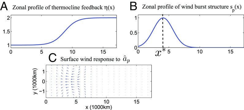
The above model retains a few essential processes that model the ENSO dynamics in a simple fashion. Latent heating , proportional to SST, is depleted from the ocean and forces an atmospheric circulation. The resulting zonal wind stress in return forces an ocean circulation that imposes feedback on the SST through thermocline depth anomalies . This thermocline feedback is more significant in the eastern Pacific, as shown in Fig. 1.
Fig. 1.
(A–C) Profiles of (A) the thermocline coefficient , (B) the zonal structure of the wind burst with its peak at , and (C) the surface wind response in the equatorial Pacific band (from 15°S to 15°N) to a mean easterly trade wind anomaly .
The coupled model introduces unique theoretical elements such as a nondissipative atmosphere consistent with the skeleton model for the Madden–Julian oscillation (MJO) (38, 39), valid here on the interannual timescale and suitable to describe the dynamics of the Walker circulation (40–42). In addition, the meridional axes and are different in the atmosphere and ocean as they each scale to a suitable Rossby radius. This allows for a systematic meridional decomposition of the system into the well-known parabolic cylinder functions (43), which keeps the system low dimensional (44). Here, models 1–3 are projected and truncated to the first parabolic cylinder function of the atmosphere (38) and the ocean (1), respectively. Details are included in SI Appendix.
The coupled system in Eqs. 1–4 without the nonlinear zonal advection in Eq. 3 was systematically studied in ref. 33. It succeeds in recovering the traditional El Niño with occasionally super El Niño and capturing the ENSO statistics in the eastern Pacific as in nature. If the stochastic wind burst is further removed, the resulting coupled system is linear, deterministic, and stable. Therefore, such a coupled model is fundamentally different from the Cane–Zebiak model (30) and other nonlinear models (31, 32) where the internal instability rather than the external wind bursts plays the role of triggering the ENSO cycles.
The observational significance of the zonal advection has been shown for the CP El Niño (5, 45). Different from the previous works (46, 47) where the advection is mostly linear and requires ad hoc parameterization of the background SST gradient, a simple nonlinear advection is adopted in Eq. 3 that contributes significantly to the SST tendency. Such nonlinear advection provides the mechanism of transporting anomalous warm water to the central Pacific region by the westward ocean zonal current. Importantly, when stochasticity is included in the wind activity , this nonlinear zonal advection involves the contribution from both mean and fluctuation, the latter of which is usually ignored in the previous works. The combined effect of this nonlinear advection, a mean easterly trade wind anomaly, and effective stochastic noise was shown to facilitate the intermittent occurrence of the CP El Niño with realistic features (34).
Stochastic Wind Burst Process.
Stochastic parameterization of the wind activity is added to the model that represents several important ENSO triggers such as westerly wind bursts (WWBs) (28, 29, 48) and easterly wind bursts (EWBs) (49) as well as the convective envelope of the MJO (27, 50). It also includes the recent multidecadal strengthening of the easterly trade wind anomaly. The wind bursts read as
| [5] |
with amplitude and fixed zonal spatial structure shown in Fig. 1. Here, equals the first parabolic cylinder function of the atmosphere (SI Appendix). Both the wind burst perturbations (29) and the strengthening of the trade wind anomaly (12, 13) are localized over the western equatorial Pacific according to the observations and for simplicity they share the same zonal extent.
The evolution of wind burst amplitude reads as
| [6] |
where is dissipation and is a white-noise source, representing the intermittent nature of the wind bursts at an interannual timescale. The amplitude of the wind burst noise source depends on (Eq. 7), which is the average of SST anomalies in the western half of the equatorial Pacific (). Note that this state-dependent wind amplitude has a different viewpoint from those in previous works (37, 51, 52) that rely on the eastern Pacific SST. The term represents the mean strengthening of the easterly trade wind anomaly. Corresponding to , the direct response of the surface wind associated with the Walker circulation at the equatorial Pacific band is shown in Fig. 1C, which is similar to the observed intensification of the Walker circulation in recent decades (12, 13).
A Three-State Markov Jump Process.
Due to the fact that the ENSO diversity is associated with the wind activity with distinct features (33, 34), a three-state Markov jump process (53–55) is adopted to model the wind activity. Here, state 2 primarily corresponds to the traditional El Niño and state 1 to the CP El Niño whereas state 0 represents discharge and quiescent phases. The following criteria are used in determining the parameters in Eq. 6 in each state. First, strong wind bursts play an important role in triggering the traditional El Niño (27–29), which suggests a large noise amplitude in state 2. Second, the observational fact that an enhanced easterly trade wind has accompanied the CP El Niño since the 1990s indicates a negative (easterly) mean in state 1. To obtain the CP El Niño, the amplitude of and the stochastic noise must be balanced (34). This implies a moderate noise amplitude in state 1, which also agrees with observations (56). Finally, only weak wind activity is allowed in the quiescent state and the discharge phase with La Niña (state 0). Thus, the three states are given by
| [7] |
respectively, where represents a relaxation time around d. Note that the same mean easterly trade wind anomaly as in state 1 is adopted in state 2 due to the fact that both the traditional and the CP El Niño occurred during the last 25 y. Because the amplitude of the stochastic noise dominates the mean easterly wind in state 2, this mean state actually has little impact on simulating the traditional El Niño events. On the other hand, to guarantee no El Niño event occurring in the quiescent phase, no mean trade wind anomaly is imposed in state 0. With such a choice of the parameters, both the amplitude and the timescale of the wind burst activity are similar to those in nature.
The local transition probability from state to State with for small is defined as
| [8] |
and the probability of staying in state is given by
| [9] |
Importantly, the transition rates (with ) depend on , implying the state dependence of the wind bursts (57–59). A transition (with ) from a less active to a more active state is more likely when and vice versa. This allows, for example, a rapid shutdown of wind burst activity followed by extreme El Niño events, as in nature.
The transition rates are chosen in accordance with the observational record. A higher transition probability from state 2 to state 0 is adopted compared with that to state 1, representing the situation that the traditional El Niño is usually followed by the La Niña rather than the CP El Niño (e.g., years 1963, 1965, 1972, 1982, 1987, and 1998). Likewise, starting from the quiescent phase, the model has a preference toward the occurrence of the CP El Niño rather than the eastern Pacific super El Niño, as observed in years 1968, 1990, and 2001. See SI Appendix for details. It is also shown in SI Appendix that the model statistics are robust with respect to the perturbation of the parameters, which indicates that a crude estimation of the transition rates is sufficient for obtaining the ENSO diversity with realistic features.
The parameterization of the wind activity in Eqs. 5–9 emphasizes the distinct properties of the wind activity at different ENSO phases and describes effective state-dependent transitions in a simple and effective fashion. It is different from those adopted in previous works that involve many detailed structures, such as the central location and peak time of each wind burst event (29, 35, 36) and the separation of the linear and nonlinear parts of the wind activity (37).
Results
Now we present the statistical diversity of ENSO produced by the coupled model. To compare the model simulations with the observational record, we define three indexes from the model simulations: T-3, T-3.4, and T-4, which are the averaged SSTs over the regions of Niño 3 (150W–90W), Niño 3.4 (170W–120W), and Niño 4 (160E–150W), respectively.
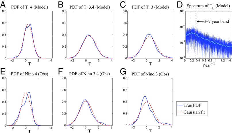
Fig. 2 shows the probability density functions (PDFs) of T-4, T-3.4, and T-3 as well as the power spectrum of , which is the averaged SST over the eastern Pacific. These statistics are formed based on a -y-long model simulation. The power spectrum of peaks at the interannual band (3–7 y), which is consistent with that in nature (60). The variance of all three T indexes almost perfectly matches those of the three Niño indexes (from the NOAA). Particularly, the fact that the variance of SST in the Niño 4 region is roughly half that in the other two regions is captured by the coupled model. In addition, consistent with observations, the PDFs of T-4 and T-3 show negative and positive skewness, respectively. The presence of a fat tail together with the positive skewness in T-3 indicates the extreme El Niño events in the eastern Pacific (61). Note that, despite the correct skewed direction, the skewness of T-3 seems to be underestimated compared with that in Niño 3. However, the Niño indexes are calculated based only on a 34-y-long monthly time series (1982/01–2016/02), which may not be sufficient to form unbiased statistics. In fact, the single super El Niño event during 1997–1998 accounts for a large portion of the skewness in Niño 3. Therefore, the statistics of the model are qualitatively consistent with those in nature. SI Appendix contains sensitivity tests, which show that the model statistics are robust to parameter variations.
Fig. 2.
PDFs of T-3, T-3.4, and T-4 from the coupled model (A–C) and those of Niño 3, 3.4, and 4 from the National Oceanic and Atmospheric Administration (NOAA) observational record (1982/01–2016/02) (E–G). D shows the power spectrum of . The model statistics are computed based on a -y-long simulation.
These non-Gaussian statistics indicate the significant role of both the nonlinear zonal advection and the state-dependent noise in the wind burst process, because otherwise the PDFs of T indexes will all become Gaussian. In addition, in the absence of the CP El Niño, positive skewness is found in T-4 from the coupled model (33).
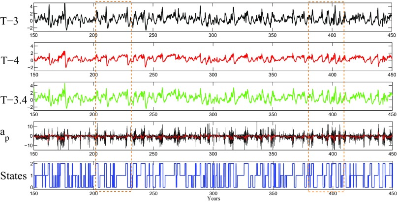
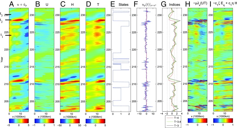
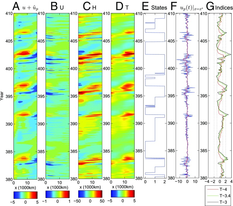
Fig. 3 shows the time series of the three T indexes, the stochastic wind amplitude , and the state transitions. Examples of the ENSO diversity are demonstrated in Figs. 4 and 5. First, the coupled model succeeds in simulating traditional El Niño events in the eastern Pacific including both the quasi-regular moderate El Niño (e.g., ) and the super El Niño (e.g., ). These traditional El Niño events are typically followed by a reversal of conditions toward La Niña with weaker strengths but longer durations. Particularly, the super El Niño appears roughly every 15–25 y (T-3 index), as in nature. These traditional El Niño events start with a realistic buildup of SST and thermocline depth anomalies in the western Pacific in the preceding year, which switches the system to the active state (state 2) and increases wind burst activity over the warm pool region. At the onset phase of these El Niño events, a strong series of WWBs (Fig. 4F) triggers enhanced thermocline depth and SST anomalies in the western Pacific, which then propagate eastward and intensify in the eastern Pacific at the peak of the El Niño events. Meanwhile, the western edge of the warm pool is cooled (62). However, there are many phases (e.g., ) where wind burst activity builds up without triggering an El Niño event, implying that wind burst activity in the model is a necessary but nonsufficient condition for the El Niño development (52, 63–65). In Fig. 4, there is also a special event around that resembles the observational record in year 2014. That is, a strong WWB tends to trigger a traditional El Niño. However, an intense EWB occurs right after the WWB, which serves as the key dynamical factor that stalled the El Niño development (49). On the other hand, in the presence of the mean easterly wind anomaly and moderate wind activity, CP El Niño events are simulated by the coupled model (state 1), where the duration of these CP El Niño events varies from 1–2 y (e.g., ) to 4–5 y (e.g., –). Particularly, the period from to resembles the observed ENSO episode during the 1990s, where a series of 5-y CP El Niño events is followed by a super El Niño and then a La Niña.
Fig. 3.
A sample period-series T-3, T-4, T-3.4; the stochastic wind activity amplitude ; and the states in the Markov process. The red curve on top of shows the 120-d running average indicating the low-frequency part of the wind activity. The two dashed boxes correspond to the periods shown in Figs. 4 and 5.
Fig. 4.
Period from to in Fig. 3. (A–D) Hovmoller diagram of atmospheric wind , ocean zonal current , thermocline depth , and SST anomaly . (E–G) Transitions of the states, stochastic wind , and its 120-d running average (red) at the longitude with its maximum value and T indexes. (H and I) Budget of flux divergence and the summation of latent heating and thermocline feedback . All variables shown are at the equator.
Fig. 5.
Same as A–G in Fig. 4 but from to .
Budget analysis indicates the distinct mechanisms of the two types of El Niño in the coupled model. The flux divergence appears to be the main contributor to the occurrence of the CP El Niño, where the westward anomalous zonal ocean current tends to transport the anomalous warm water to the central Pacific region and leads to the eastern Pacific cooling with a shallow thermocline depth (Fig. 4 H and I from to ). On the other hand, the dominant factor for the traditional El Niño is the thermocline feedback , which is nearly proportional to the SST in the eastern Pacific and dominates the budget of the SST tendency (Fig. 4 C, D, and I around and t = ). All these findings in the model recover the analysis from the observational data (3, 8–11).
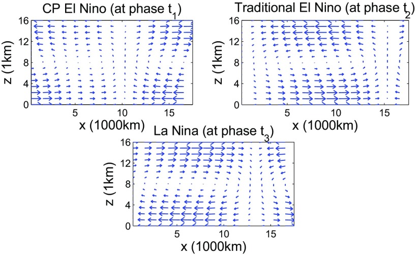
Fig. 6 shows the anomalous Walker circulations at three different ENSO phases, which all agree with the observational record (5). Particularly, the surface wind converges and forms the rising branch of the circulation in the central and eastern Pacific at the CP and the traditional El Niño phases ( and ), respectively. On the other hand, at the La Niña phase , a descending branch of the anomalous Walker cell is found in the eastern Pacific, along with the divergence of the surface wind.
Fig. 6.
Anomalous Walker circulation at different phases shown in Fig. 4.
Conclusions
A simple dynamical model is developed that automatically captures key features and the statistical diversity of ENSO. Systematic strategies are designed for incorporating several major causes of the ENSO diversity into a simple coupled ocean–atmosphere model that is otherwise deterministic, linear, and stable. First, a stochastic parameterization of the wind bursts including both westerly and easterly wind is coupled to the ocean–atmosphere system, where the amplitude of the wind bursts depends on the SST in the western Pacific warm pool. Second, a simple nonlinear zonal advection and a mean easterly trade wind anomaly are incorporated into the coupled system that enables anomalous warm SST in the central Pacific. Finally, an effective three-state stochastic Markov jump process is developed to drive the stochastic wind activity, which allows the occurrence of different types of ENSO.
The statistics produced by the coupled model resemble those in nature. The power spectrum of peaks at the interannual band. The variance of the three T indexes almost perfectly matches those in the observational record of Niño 3, 3.4, and 4 indexes and the directions of the skewness of the T and the Niño indexes are the same in all three regions. Importantly, the fat tail together with the positive skewness in the PDF of the T-3 index implies the intermittent occurrence of the extreme El Niño events. The coupled model succeeds in simulating both the CP and the traditional El Niño events, including quasi-regular moderate El Niño and super El Niño, as well as the La Niña with realistic features. Particularly, the model is able to reproduce the observed ENSO episode with diversity in the 1990s. In addition, the anomalous Walker circulations at different ENSO phases all resemble those in nature.
Supplementary Material
Acknowledgments
The research of A.J.M. is partially supported by the Office of Naval Research Grant Office of Naval Research, Multidisciplinary University Research Initiative (ONR MURI) N00014-16-1-2161 and the New York University Abu Dhabi Research Institute. N.C. is supported as a postdoctoral fellow through A.J.M.’s ONR MURI Grant. The authors thank the National Oceanic and Atmospheric Administration for providing Niño indexes.
Footnotes
The authors declare no conflict of interest.
This article contains supporting information online at www.pnas.org/lookup/suppl/doi:10.1073/pnas.1620766114/-/DCSupplemental.
References
- 1.Clarke AJ. An Introduction to the Dynamics of El Nino & the Southern Oscillation. Academic; Cambridge, MA: 2008. [Google Scholar]
- 2.Lee T, McPhaden MJ. Increasing intensity of El Niño in the central-equatorial Pacific. Geophys Res Lett. 2010;37(14):L14603. [Google Scholar]
- 3.Kao H-Y, Yu J-Y. Contrasting eastern-Pacific and central-Pacific types of ENSO. J Clim. 2009;22(3):615–632. [Google Scholar]
- 4.Ashok K, Behera SK, Rao SA, Weng H, Yamagata T. El Nino Modoki and its possible teleconnections. J Geophys Res. 2007;112:C11007. [Google Scholar]
- 5.Kug JS, Jin FF, An SI. Two types of El Niño events: Cold tongue El Niño and warm pool El Niño. J Clim. 2009;22(6):1499–1515. [Google Scholar]
- 6.Larkin NK, Harrison D. On the definition of El Niño and associated seasonal average US weather anomalies. Geophys Res Lett. 2005;32(13):L13705. [Google Scholar]
- 7.Guilyardi E. El Nino–mean state–seasonal cycle interactions in a multi-model ensemble. Clim Dyn. 2006;26(4):329–348. [Google Scholar]
- 8.Yu J-Y, Kao H-Y. Decadal changes of ENSO persistence barrier in SST and ocean heat content indices: 1958–2001. J Geophys Res Atmos. 2007;112(D13):D13106. [Google Scholar]
- 9.Yeh S-W, et al. El Niño in a changing climate. Nature. 2009;461(7263):511–514. doi: 10.1038/nature08316. [DOI] [PubMed] [Google Scholar]
- 10.Yeh S-W, Kug J-S, An S-I. Recent progress on two types of El Niño: Observations, dynamics, and future changes. Asia Pac J Atmos Sci. 2014;50(1):69–81. [Google Scholar]
- 11.Ren H-L, Jin F-F. Recharge oscillator mechanisms in two types of ENSO. J Clim. 2013;26(17):6506–6523. [Google Scholar]
- 12.England MH, et al. Recent intensification of wind-driven circulation in the Pacific and the ongoing warming hiatus. Nat Clim Chang. 2014;4(3):222–227. [Google Scholar]
- 13.Sohn B, Yeh S-W, Schmetz J, Song H-J. Observational evidences of Walker circulation change over the last 30 years contrasting with GCM results. Clim Dyn. 2013;40(7-8):1721–1732. [Google Scholar]
- 14.Merrifield MA, Maltrud ME. Regional sea level trends due to a Pacific trade wind intensification. Geophys Res Lett. 2011;38(21):L21605. [Google Scholar]
- 15.L’Heureux ML, Lee S, Lyon B. Recent multidecadal strengthening of the Walker circulation across the tropical Pacific. Nat Clim Chang. 2013;3(6):571–576. [Google Scholar]
- 16.Choi J-W, Kim I-G, Kim J-Y, Park C-H. The recent strengthening of Walker circulation. SOLA. 2016;12(0):96–99. [Google Scholar]
- 17.McGregor S, et al. Recent Walker circulation strengthening and Pacific cooling amplified by Atlantic warming. Nat Clim Chang. 2014;4(10):888–892. [Google Scholar]
- 18.Weng H, Behera SK, Yamagata T. Anomalous winter climate conditions in the Pacific Rim during recent El Niño Modoki and El Niño events. Clim Dyn. 2009;32(5):663–674. [Google Scholar]
- 19.Capotondi A, et al. Understanding ENSO diversity. Bull Am Meteorol Soc. 2015;96(6):921–938. [Google Scholar]
- 20.Ham YG, Kug JS. How well do current climate models simulate two types of El Nino? Clim Dyn. 2012;39(1-2):383–398. [Google Scholar]
- 21.Kug J-S, Ham Y-G, Lee J-Y, Jin F-F. Improved simulation of two types of El Niño in CMIP5 models. Environ Res Lett. 2012;7(3):034002. [Google Scholar]
- 22.Ault TR, Deser C, Newman M, Emile-Geay J. Characterizing decadal to centennial variability in the equatorial Pacific during the last millennium. Geophys Res Lett. 2013;40(13):3450–3456. [Google Scholar]
- 23.Kim ST, Yu J-Y. The two types of ENSO in CMIP5 models. Geophys Res Lett. 2012;39(11):L11704. [Google Scholar]
- 24.Yu J-Y, Kim ST. Identification of central-Pacific and eastern-Pacific types of ENSO in CMIP3 models. Geophys Res Lett. 2010;37(15):L08706. [Google Scholar]
- 25.Wittenberg AT. Are historical records sufficient to constrain ENSO simulations? Geophys Res Lett. 2009;36(12):L12702. [Google Scholar]
- 26.Kug J-S, Choi J, An S-I, Jin F-F, Wittenberg AT. Warm pool and cold tongue El Niño events as simulated by the GFDL 2.1 coupled GCM. J Clim. 2010;23(5):1226–1239. [Google Scholar]
- 27.Hendon HH, Wheeler MC, Zhang C. Seasonal dependence of the MJO-ENSO relationship. J Clim. 2007;20(3):531–543. [Google Scholar]
- 28.Vecchi GA, Harrison DE. Tropical Pacific sea surface temperature anomalies, El Nino, and equatorial westerly wind events. J Clim. 2000;13(11):1814–1830. [Google Scholar]
- 29.Tziperman E, Yu L. Quantifying the dependence of westerly wind bursts on the large-scale tropical Pacific SST. J Clim. 2007;20(12):2760–2768. [Google Scholar]
- 30.Zebiak SE, Cane MA. A model El Niño-Southern oscillation. Mon Weather Rev. 1987;115(10):2262–2278. [Google Scholar]
- 31.Jin F-F. An equatorial ocean recharge paradigm for ENSO. Part I: Conceptual model. J Atmos Sci. 1997;54(7):811–829. [Google Scholar]
- 32.Timmermann A, Jin F-F, Abshagen J. A nonlinear theory for El Niño bursting. J Atmos Sci. 2003;60(1):152–165. [Google Scholar]
- 33.Thual S, Majda AJ, Chen N, Stechmann SN. Simple stochastic model for El Niño with westerly wind bursts. Proc Natl Acad Sci USA. 2016;113(37):10245–10250. doi: 10.1073/pnas.1612002113. [DOI] [PMC free article] [PubMed] [Google Scholar]
- 34.Chen N, Majda AJ. Simple dynamical models capturing the key features of the central Pacific El Niño. Proc Natl Acad Sci USA. 113(42):11732–11737. doi: 10.1073/pnas.1614533113. [DOI] [PMC free article] [PubMed] [Google Scholar]
- 35.Gebbie G, Tziperman E. Predictability of SST-modulated westerly wind bursts. J Clim. 2009;22(14):3894–3909. [Google Scholar]
- 36.Gebbie G, Eisenman I, Wittenberg A, Tziperman E. Modulation of westerly wind bursts by sea surface temperature: A semistochastic feedback for ENSO. J Atmos Sci. 2007;64(9):3281–3295. [Google Scholar]
- 37.Levine AF, Jin FF. A simple approach to quantifying the noise–ENSO interaction. Part I: Deducing the state-dependency of the windstress forcing using monthly mean data. Clim Dyn. 2015;48:1–18. [Google Scholar]
- 38.Majda AJ, Stechmann SN. The skeleton of tropical intraseasonal oscillations. Proc Natl Acad Sci USA. 2009;106(21):8417–8422. doi: 10.1073/pnas.0903367106. [DOI] [PMC free article] [PubMed] [Google Scholar]
- 39.Majda AJ, Stechmann SN. Nonlinear dynamics and regional variations in the MJO skeleton. J Atmos Sci. 2011;68(12):3053–3071. [Google Scholar]
- 40.Majda AJ, Klein R. Systematic multiscale models for the tropics. J Atmos Sci. 2003;60(2):393–408. [Google Scholar]
- 41.Stechmann SN, Ogrosky HR. The Walker circulation, diabatic heating, and outgoing longwave radiation. Geophys Res Lett. 2014;41(24):9097–9105. [Google Scholar]
- 42.Stechmann SN, Majda AJ. Identifying the skeleton of the Madden–Julian oscillation in observational data. Mon Weather Rev. 2015;143(1):395–416. [Google Scholar]
- 43.Majda A. Introduction to PDEs and Waves for the Atmosphere and Ocean. Vol 9 American Mathematical Society; Providence, RI: 2003. [Google Scholar]
- 44.Thual S, Thual O, Dewitte B. Absolute or convective instability in the equatorial Pacific and implications for ENSO. Q J R Meteorol Soc. 2013;139(672):600–606. [Google Scholar]
- 45.Su J, Li T, Zhang R. The initiation and developing mechanisms of central Pacific El Niños. J Clim. 2014;27(12):4473–4485. [Google Scholar]
- 46.Jin F-F, An S-I. Thermocline and zonal advective feedbacks within the equatorial ocean recharge oscillator model for ENSO. Geophys Res Lett. 1999;26(19):2989–2992. [Google Scholar]
- 47.Dewitte B, Yeh S-W, Thual S. Reinterpreting the thermocline feedback in the western-central equatorial Pacific and its relationship with the ENSO modulation. Clim Dyn. 2013;41(3-4):819–830. [Google Scholar]
- 48.Harrison DE, Vecchi GA. Westerly wind events in the Tropical Pacific, 1986–95*. J Clim. 1997;10(12):3131–3156. [Google Scholar]
- 49.Hu S, Fedorov AV. Exceptionally strong easterly wind burst stalling El Niño of 2014. Proc Natl Acad Sci USA. 2016;113(8):2005–2010. doi: 10.1073/pnas.1514182113. [DOI] [PMC free article] [PubMed] [Google Scholar]
- 50.Puy M, Vialard J, Lengaigne M, Guilyardi E. Modulation of equatorial Pacific westerly/easterly wind events by the Madden–Julian oscillation and convectively-coupled Rossby waves. Clim Dyn. 2016;46(7-8):2155–2178. [Google Scholar]
- 51.Jin F-F, Lin L, Timmermann A, Zhao J. Ensemble-mean dynamics of the ENSO recharge oscillator under state-dependent stochastic forcing. Geophys Res Lett. 2007;34(3):L03807. [Google Scholar]
- 52.Levine AFZ, Jin F-F. Noise-induced instability in the ENSO recharge oscillator. J Atmos Sci. 2010;67(2):529–542. [Google Scholar]
- 53.Gardiner CW, et al. Handbook of Stochastic Methods. Vol 3 Springer; Berlin: 1985. [Google Scholar]
- 54.Lawler GF. Introduction to Stochastic Processes. CRC; Boca Raton, FL: 2006. [Google Scholar]
- 55.Majda AJ, Harlim J. Filtering Complex Turbulent Systems. Cambridge Univ Press; Cambridge, UK: 2012. [Google Scholar]
- 56.Chen D, et al. Strong influence of westerly wind bursts on El Niño diversity. Nat Geosci. 2015;8(5):339–345. [Google Scholar]
- 57.Levine A, Jin FF, McPhaden MJ. Extreme noise-extreme El Niño: How state-dependent noise forcing creates El Niño-La Niña asymmetry. J Clim. 2016;29(15):5483–5499. [Google Scholar]
- 58.Lopez H, Kirtman BP. Westerly wind bursts and the diversity of ENSO in CCSM3 and CCSM4. Geophys Res Lett. 2013;40(17):4722–4727. [Google Scholar]
- 59.Lopez H, Kirtman BP, Tziperman E, Gebbie G. Impact of interactive westerly wind bursts on CCSM3. Dyn Atmos Oceans. 2013;59:24–51. [Google Scholar]
- 60.Kleeman R. Stochastic theories for the irregularity of ENSO. Philos Trans A Math Phys Eng Sci. 2008;366(1875):2509–2524. doi: 10.1098/rsta.2008.0048. [DOI] [PubMed] [Google Scholar]
- 61.Burgers G, Stephenson DB. The “normality” of El Niño. Geophys Res Lett. 1999;26(8):1027–1039. [Google Scholar]
- 62.Cronin MF, McPhaden MJ. The upper ocean heat balance in the western equatorial Pacific warm pool during September–December 1992. J Geophys Res Oceans. 1997;102(C4):8533–8553. [Google Scholar]
- 63.Hu S, Fedorov AV, Lengaigne M, Guilyardi E. The impact of westerly wind bursts on the diversity and predictability of El Niño events: An ocean energetics perspective. Geophys Res Lett. 2014;41(13):4654–4663. [Google Scholar]
- 64.Fedorov AV, Hu S, Lengaigne M, Guilyardi E. The impact of westerly wind bursts and ocean initial state on the development, and diversity of El Niño events. Clim Dyn. 2015;44(5-6):1381–1401. [Google Scholar]
- 65.Roulston MS, Neelin JD. The response of an ENSO model to climate noise, weather noise and intraseasonal forcing. Geophys Res Lett. 2000;27(22):3723–3726. [Google Scholar]
Associated Data
This section collects any data citations, data availability statements, or supplementary materials included in this article.


