Probabilistic Modeling of Imaging, Genetics and Diagnosis

Abstract

We propose a unified Bayesian framework for detecting genetic variants associated with disease by exploiting image-based features as an intermediate phenotype. The use of imaging data for examining genetic associations promises new directions of analysis, but currently the most widely used methods make sub-optimal use of the richness that these data types can offer. Currently, image features are most commonly selected based on their relevance to the disease phenotype. Then, in a separate step, a set of genetic variants is identified to explain the selected features. In contrast, our method performs these tasks simultaneously in order to jointly exploit information in both data types. The analysis yields probabilistic measures of clinical relevance for both imaging and genetic markers. We derive an efficient approximate inference algorithm that handles the high dimensionality of image and genetic data. We evaluate the algorithm on synthetic data and demonstrate that it outperforms traditional models. We also illustrate our method on Alzheimer’s Disease Neuroimaging Initiative data.

I. Introduction

In this paper, we propose a probabilistic model to discover genetic variants associated with a disease using image data as an intermediate phenotype. The search for genetic variants that increase the risk of a particular disorder is one of the central challenges in medical research, and has been traditionally performed via genome-wide association studies (GWAS). In GWAS, it is common to examine the associations of genetic variants with disease by performing a univariate analysis between the disease incidence and each genetic marker independently. However, testing one variant at a time does not fully realize the potential of GWAS because some genetic variants may have a weak but cumulative effect that is neglected by a univariate method [1], [2]. Imaging genetics introduces image-based biomarkers as a promising intermediate phenotype¹ (i.e., endo-phenotype) between genetic variants and diagnosis. Given that in some pathologies, such as the Alzheimer’s disease, imaging features have strong correlation with the clinical diagnosis and can offer a clearer picture of the association [5], [6], it is beneficial to exploit them to improve the associations of weak genetic markers. Furthermore, in contrast to a binary diagnosis, imaging data contains many variations caused by a disease which helps to stratify the disease population in more informative ways.

Imaging genetics presents numerous challenges in clinical studies due to the relatively small number of subjects and extremely high dimensionality of images (hundreds of thousands of voxels) and genetic data (millions of single nucleotide polymorphisms (SNPs)). To address the problem of high dimensionality and small sample size, earlier methods considered only a few imaging candidates (voxels, regions, or other biomarkers) or only a few genetic markers in the analysis [7], [8]. The reduced joint dataset was then analyzed in a univariate framework, where pairs of a candidate genetic variant and an imaging biomarker were tested for association via standard statistical tests. Examples include using activation maps of the prefrontal cortex to find SNPs associated with schizophrenia [8] and searching for changes in regional gray matter volumes correlated with the genetic risk of Alzheimer’s disease [7], [9].

More recently, genome-wide voxel-wise analysis has been demonstrated using univariate methods [10]. However, massive univariate analysis has several limitations. Due to multiple comparisons, a conservative corrected significance level is selected to limit the false positive rate, but this correction dramatically reduces the power of the test. Moreover, the univariate methods are unlikely to identify weaker variants that jointly create an additive effect. Multivariate techniques aim to overcome short-comings of univariate analysis [11], [12].

A common approach is to use a multivariate regression combined with a regularization to extract a sparse set of coefficients for correlated genetic variants and image features. Various forms of relationship between imaging and genetic data along with different regularization terms have been proposed in the literature. For example, it is common to assume that image and genetic data lie in a joint hidden (latent) space. This is equivalent of enforcing different forms of low rank regularization on data: sparse reduced rank regression (sRRR) [12], [13], Partial Least Squares (PLS)[11] or Canonical Correlation Analysis (CCA) [11]. Unfortunately, these unsupervised methods do not use the clinical labels (e.g., diagnosis) directly, and thus the detected genetic markers and image features are not immediately related to the disease of interest. The image features relevant to the disease are selected separately by modeling the relationship between image features and the phenotype of interest. For example, sRRR has been demonstrated using brain regions pre-selected for Alzheimer’s disease (AD) via Linear Discriminant Analysis [13].

In contrast, we model and estimate relevant genetic variants in the context of abnormal variations that are characterized by imaging features. Our method is broadly applicable to any imaging biomarker, such as anatomical regions, tissue appearance, or functional measures. Here, we demonstrate our method in application to Alzheimer’s disease, and use thickness of cortical regions and the volume of sub-cortical structures as image features.

We define a probabilistic model to encode the relationship among genetic, image and disease measures. Our model incorporates a common assumption made by genetic studies that only a small set of genetic variants is associated with any particular disease, leading to sparsity-inducing priors. The relevant subset of genetic markers induces variation in certain image-based features, and a subset of these measures exhibits changes that are discriminative with respect to the disease phenotype. Therefore, in our model if a brain region is irrelevant for the target disease, it is ignored even if it is strongly modulated by genetics. We also derive an efficient inference algorithm to identify relevant brain regions and genetic loci, and demonstrate the method on synthetic data and real data from the ADNI study [14]. We demonstrate that our algorithm outperforms standard univariate and regression analyses for genetic variant detection on synthetic data and yields promising results in a real clinical study. This paper extends our publication of the preliminary results [15] by deriving a novel robust inference algorithm. It also expands the empirical evaluation.

The remainder of this paper is organized as follows. In the next section, we build a graphical model that captures the relationship among image, genetic and diagnostic variables. In Section III, we propose an efficient algorithm to perform inference of the model. Derivation details are discussed in the Appendix in the supplementary file. Sections IV and V report experimental results on simulated and real data, respectively. We conclude the paper with a discussion of the results and future directions in Section VI.

II. Method

A. Notations and Terminology

Throughout this paper, we use regular fonts (e.g., x, τ) and bold fonts (e.g., x, τ) to denote scalar and vector, respectively. Some uppercase letters are reserved for the number of elements: e.g., N is the number of subjects, M is the number of image regions, and S is the number of SNPs. In such cases, their lowercase counterparts are used for enumeration: e.g., subject n, image region m, and SNP s. Uppercase bold letters are used to denote matrix variables (e.g., V ∈ ℝ^S×M); in such case V_m and V_s: denote the column m and row s of the matrix V, respectively. We use V_sm to refer to the entry in the row s and column m of V. Superscripts are used to denote iterations of the algorithm (e.g., b^t) or transpose (e.g., X^T). 𝔼[·] and p(·) denote expectation and density. Table I summarizes all variables used throughout this paper.

TABLE I.

Notation and Variables Used Throughout the Paper

Model Variables: Image to Disease Phenotype
xnm	Image feature m in subject n (brain endophenotype featue).
yn	Disease phenotype (diagnosis variable/class label) of subject n: −1 - healthy, 1 - diseased.
bm ∈ {0,1}	Indicator variable that selects image feature m.
f	Latent function drawn from a Gaussian Process to predict y from image feature vector x.
β	Prior probability for selecting image features.
Model Variables: Genetics to Image
gn,s	Genetic variant s in subject n.
ωm	Regression coefficient vector for predicting image feature m using the genotype.
asm ∈ {0,1}	Indicator variable that selects SNP s for modeling image feature in region m.
α	Prior probability for selecting genetic variants.
${\sigma }_{\mathit{\omega }}^2$	Variance of an element in ωm.
${\sigma }_0^2$	Variance of noise in the genetics to image regression for the relevant regions.
Variational Variables
ρm	Posterior probability of selecting feature m.
τs	Posterior probability of selecting SNP s.
ν, ς	Mean and variance parameters of the genetics-to-image regression.

B. Model

We are motivated by anatomical brain studies with binary phenotypes (−1 or 1), but the analysis applies to any biomarker derived from images and the constraint on the phenotype can be easily relaxed. We assume that a study contains N individuals, each with three measurements:

• disease phenotype y ∈ {−1,1} that indicates healthy vs. disease;

• image measurements, x ∈ ℝ^M, which are usually referred to as “intermediate phenotype”. In the context of AD, image features include volume or thickness measurements of M brain structures.

• genetic variants g ∈ ℝ^S at S locations along the genome;

We assume that a subset of image features is modulated by genetics and is closely related to the disease phenotype. Detecting and utilizing such imaging features can improve the detection of relevant genetic variants.

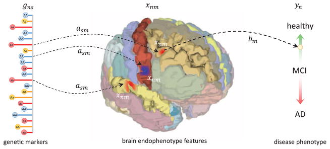
We model two types of relationships, illustrated Fig. 1: 1) the association of a subset of brain regions with the diagnosis variable y, which can be quantified by the quality of the disease prediction from image features; 2) a modulation of each image feature by the genotype. A common approach is to consider these two relationships separately, selecting relevant brain structures and then performing a statistical test (e.g., t-test or sparse regression) to identify the relevant genotype [13]. In contrast, we propose a model to perform these two steps jointly, via two coupled regression models:

Fig. 1.

A schematic illustration of the relationship between genetic, imaging and clinical measures in our model.

• A sparse subset of imaging features selected by b ∈ {0,1}^M is related to the diagnosis variable y via a logistic regression model. For each region, we model its elements (i.e., b_m) using a Bernoulli distribution (Section II-C).

• Variations in image features for region m can be explained by a sparse subset of the genotype which is selected by a_m ∈ {0,1}^S. Similarly, we model its elements (i.e., a_sm) via a Bernoulli distribution (Section II-D).

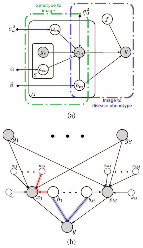
We treat the indicator variables ${\{{\mathbf{a}}_m\}}_{m=1}^M$ and b as latent. The graphical model in Fig. 2 presents the relationships among all variables in the model. One can view the model shown in Fig. 2 as two-layers of regression that share latent variables for the image data. Below, we first define the relationship between image features and the disease phenotype and then specify the generative model for the relationship between SNPs and image features. We do not model a direct link between genetic variants and disease label. It is captured indirectly through image features. The general idea is illustrated in Fig. 1.

Fig. 2.

(a) Graphical representation of the generative model. Hollow circles (○) denote random variables, small solid circles (●) represent hyper-parameters, and shaded circles represent observed variables. The black plates indicate conditionally independent instantiations. More specifically, α, β, σ_ω and σ₀ are the hyper-parameters. The dashed boxes illustrate the different parts of the model. (b) Instead of plates, the repetition of the random variables are shown explicitly. To avoid the visual clutter, the hyper-parameters are not shown. The blue and the red paths show so-called v-structure dependence. It means that those variables are conditionally dependent hence the posterior values for those variables are related.

C. From Imaging Features to Disease Phenotype

To predict the binary class label y from a sparse set of image features x, we use a variant of the log-odds model:

$$log\left\{\frac{p(y=1\mid f,\mathbf{b},\mathbf{x})}{1-p(y=1\mid f,\mathbf{b},\mathbf{x})}\right\}=f(\mathbf{x}\odot \mathbf{b}),$$ (1)

where ⊙ is the element-wise product, b ∈ {0,1}^M is the latent variable that selects relevant regions, and f(·) is a latent stochastic function. In effect the operation x ⊙ b masks out the irrelevant features.

We assume exchangeable Bernoulli prior for b. In other words, we model selection of each region as a biased coin flip, i.e., p(b_m) = β^b_m(1 − β)^1−b_m, where β is the prior probability of including a brain region. We use the Gaussian Process (GP) as a prior for f [16]. A Gaussian Process is a random process where any finite sample set is distributed as a multi-dimensional Gaussian distribution. GP is completely defined by its prior mean and covariance functions, i.e., f(x ⊙ b) ~ 𝒢℘(m_b(x), k_b(x,x′)), where

$$\begin{array}{l}{m}_{\mathbf{b}}(\mathbf{x})=\mathbb{E}[f(\mathbf{x}\odot \mathbf{b})],\\ k_{\mathbf{b}}(\mathbf{x},{\mathbf{x}}^{\prime })=\mathbb{E}[{(f(\mathbf{x}\odot \mathbf{b})-m_{\mathbf{b}}(\mathbf{x}\odot \mathbf{b}))}^T(f({\mathbf{x}}^{\prime }\odot \mathbf{b})-m_{\mathbf{b}}({\mathbf{x}}^{\prime }))].\end{array}$$

We assume m_b(x) = 0 since y ∈ {−1,1} and we do not aim to induce a bias toward either label. The covariance function k(·,·)is the crucial part of a GP. There are several well-known choices for k(·,·)such as Linear k(x,x′) = x^Tx′, or Squared Exponential $k(\mathbf{x},{\mathbf{x}}^{\prime })=exp(-{\Vert \mathbf{x}-{\mathbf{x}}^{\prime }\Vert }_2^2/2{\sigma }^2)$. We use the linear kernel in this paper, setting k(x,x′) = x^Tx′. The expression on the left hand side of (1) specifies the likelihood (i.e., the link function). For example, a straightforward change from the logistic likelihood to a Gaussian likelihood enables modeling continuous clinical measurements (e.g., cognitive scores).

D. From Genetic Variants to Imaging Features

An imaging feature m is either relevant to the disease (b_m = 1) or not (b_m = 0). In modeling the relationship between genetics and imaging, we treat these cases differently. If feature m is irrelevant (b_m = 0), we model the variation in the region as a Gaussian distribution centered at zero with a fixed standard deviation of one: x_m ~ 𝒩(·;0, 1). This assumption is not limiting, since we can always normalize the samples to have zero mean and unit variance. The normal distribution can be replaced by a different distribution if needed. One can view this assumption as our null distribution. If feature m is relevant for disease prediction (b_m = 1), variations in the values of this feature are explained by a sparse subset of the genetic variants g ∈ ℝ^S. We define a_m ∈ {0,1}^S to be a vector of latent Bernoulli random variables that specify a subset, or mask, of relevant genetic markers for region m, and arrive at the second regression component of our model:

$$x_{nm}={\mathit{\omega }}_m^T({\mathbf{g}}_n\odot {\mathbf{a}}_m)+{\epsilon }_{nm},$$ (2)

where ω_m is the vector of regression coefficients, ${\epsilon }_{nm}~\mathcal{N}(·;0,{\sigma }_0^2)$ is the iid residual noise in the image feature m for subject n. Adopting Bayesian variable selection based on the spike-and-slab model [17], [18], we assume a Gaussian distribution with zero mean and variance σ₀σ_ω as a prior for the regression coefficient ω_m. This choice of parameterization facilitates derivations explained in the Section III. Similar to the indicator variable b that selects image features, we assume exchangeable Bernoulli distribution as a prior for a_m:

$$p(a_{sm};\alpha )={\alpha }^{a_{sm}}{(1-\alpha )}^{1-a_{sm}},$$ (3)

where α is the prior probability of including any SNP in the model.

Combining, we obtain the likelihood of the image feature m:

$$p(x_{nm}\mid b_m,{\mathbf{a}}_m,\mathbf{g};{\mathit{\omega }}_m,{\sigma }_0^2)=\{\begin{array}{ll}\mathcal{N}(x_{nm};0,1)\hfill & \text{if}{b}_m=0,\hfill \\ \mathcal{N}(x_{nm};{\mathit{\omega }}_m^T({\mathbf{g}}_n\odot {\mathbf{a}}_m),{\sigma }_0^2),\hfill & \text{if}{b}_m=1.\hfill \end{array}$$ (4)

The first line of (4) assumes a simple normal distribution as a null model. To handle cases where a non-disease related genetic variants affect a relevant region (i.e., b_m = 1), we assume that the effect of the normal genetic variants along with other covariates (e.g., age, gender, etc.) are already subtracted from the data and (4) models the normalized residual. More explicitly, we fit a regression model on all measured nuisance variables in a normal population. x_nm represents the residual of the regression which presumably regresses out all of the nuisance variables.

E. Complete Model

We define 𝒵 = {f,b,a₁,…,a_m,ω₁,…,ω_m}to be the set of latent variables, to be the set of data variables 𝒟 = {X,y}that we model, and $\pi =\{{\sigma }_0^2,{\sigma }_{\omega }^2,\alpha ,\beta \}$ to be the set of hyper-parameters. We use y = [y₁;···;y_N] to denote the set of all clinical phenotypes (class labels) X ∈ ℝ^N×M and G ∈ ℝ^N×S and are respectively image and genetic data of all subjects where each row is a subject and each column represents a measurement from one brain region (for X) or genotype from all loci (for G). Since the hyper-priors are treated slightly differently during inference, in this section we focus on the structure of the conditional probability given the hyper-parameters: p(𝒟, 𝒵|π;G) (see the Appendix in the supplementary file). Combining the elements of the model in (1)–(4), we construct the joint distribution of the hidden variables 𝒵 and modeled variables 𝒟:

$$p(\mathcal{D},\mathcal{Z}\mid \pi ;\mathbf{G})=p(f)\prod _{m=1}^{M}p({\mathit{\omega }}_m\mid \pi )p(b_m\mid \pi )\prod _{s=1}^{S}p(a_{sm}\mid \pi )\times \prod _{n=1}^{N}p(y_n\mid f,\mathbf{b},x_{nm};\pi )p(x_{nm}\mid b_m,{\mathbf{a}}_m,{\mathit{\omega }}_m;g_{ns},\pi ).$$ (5)

In the next section, we focus on specifying hyper-priors p(π).

F. Hyper-Priors

For clarity of presentation, Fig. 2 presents the model but does not specify the priors for α, β, σ₀, and σ_ω. Here we define the prior distributions for each parameter of the model.

1) Prior Over Inclusion of SNPs α

We assume the conjugate prior for α ∈ (0,1), namely a Beta distribution. The shape parameters of the Beta; distribution are chosen to ensure an almost flat distribution over the entire interval (0,1) as illustrated in the experimental section.

2) Prior Over Variance of Residual σ₀

It is common to assume an uninformative prior distribution² for the variance of residuals [19]. An uninformative prior for σ₀ is proportional to $1/{\sigma }_0^2$, which can be achieved via an inverse Gamma distribution as the scale and shape priors approach zero [20], i.e., σ₀ ~ IG(ι₁, ι₂).

3) Prior Over σ_ω

Instead of directly imposing prior on σ_ω, we follow the approach of assuming a flat prior for Proportion of Variance Explained (PVE) in the response that consequently induces a prior on the parameter σ_ω [17], [21]. The underlying logic is that there might be a large number of SNPs with small PVE’s or small number of SNPs with large PVE’s; hence we assume a flat prior over PVE. Assuming that the columns of the genetic data matrix G are centered, the PVE of the genetic variants for image feature m is defined as follows:

$${\text{PVE}}_m:=\frac{{\sigma }_0^{-2}\frac{1}{N}{\displaystyle \sum _{n=1}^N}{({\mathbf{G}}_{n:}{\mathit{\omega }}_m)}^2}{1+{\sigma }_0^{-2}\frac{1}{N}{\displaystyle \sum _{n=1}^N}{({\mathbf{G}}_{n:}{\mathit{\omega }}_m)}^2}.$$

A rough estimate of the expectation of PVE (i.e., integrating ω_m out) can be represented to be:

$${\widehat{\text{PVE}}}_m=\frac{\alpha \frac{{\sigma }_{\omega }^2}{{\sigma }_0^2}\varrho }{\left(1+\alpha \frac{{\sigma }_{\omega }^2}{{\sigma }_0^2}\varrho \right)},$$ (6)

where $\varrho =(1/N){\sum }_{n=1}^N{\sum }_{s=1}^S{g}_{ns}^2$ is the sum of the sample variances of the genetic data at all S loci. We assume a uniform prior over $\widehat{\text{PVE}}$ [17]. This prior aids interpretation as it applies stronger shrinkage in models with more non-zero regression coefficients [21].

We leave the prior β for selecting image features as a non-random hyper-parameter whose effect on the final results will be studied empirically in the experimental section.

G. Joint Modeling Image and Genetics vs. Two-Step Inference

Our method jointly models imaging and genetic variations. To clarify the concept, we first explain the so-called “two-steps” method in the context of our algorithm. A two step approach (e.g., [13]) first selects a subset of brain regions (columns of X). This can be done using a univariate or multivariate approach. A univariate approach seeks a Maximum a Posterior (MAP) estimate to the following formulation accounting for each column separately:

$$\underset{\text{posterior}}{\underbrace{p(b_m\mid \mathbf{y},{\mathbf{X}}_{:,m})}}\propto \underset{\text{Likelihood}\text{term}}{\underbrace{p(\mathbf{y}\mid {\mathbf{X}}_{:,m},b_m)}}\underset{\text{prior}}{\underbrace{p(b_m)}},$$ (7)

where b_m is an indicator variable with 1 indicating relevance, and 0 not; and X_:,m is the column m of X, corresponding to the features from brain region m. Assuming uniform prior, most univariate methods find the most likely region by testing the likelihood term for b_m = 1 or b_m = 0, i.e., p(y|X_:,m, b_m = 1) ≶ p(y|X_:,m, b_m = 0).

Unlike univariate approaches, a multivariate method considers all variables at the same time to find MAP or posterior probability of this form:

$$p(\mathbf{b}\mid \mathbf{y},\mathbf{X})\propto \underset{\text{Likelihood}\text{term}}{\underbrace{p(\mathbf{y}\mid \mathbf{X},\mathbf{b})}}\underset{\text{prior}}{\underbrace{p(\mathbf{b})}},$$ (8)

where b is a m-dimensional binary hidden vector that denotes the relevance of M the image regions together.

Although the posterior value depends on all brain regions (simultaneously), such model does not account for the genetic variations. Our model specifically addresses this problem. The graphical model in Fig. 2(a) implies that the posterior probability of the brain regions takes the following form:

$$p(\mathbf{b}\mid \mathbf{y},\mathbf{X},\mathbf{G})\propto \underset{\text{Likelihood}\text{of}\text{imaging}\text{data}}{\underbrace{p(\mathbf{y}\mid \mathbf{X},\mathbf{b})}}\times \underset{\text{Posterior}\text{of}\text{the}\text{genetic}\text{to}\text{imaging}\text{model}}{\underbrace{p({\mathbf{X}}_{:,m}\mid {\{{\mathbf{a}}_m\}}_m^M;\mathbf{G})p({\mathbf{a}}_m)}}\underset{\text{prior}}{\underbrace{p(\mathbf{b})}}$$ (9)

$$logp(\mathbf{b}\mid \mathbf{y},\mathbf{X},\mathbf{G})=\underset{\text{contribution}\text{of}\text{imaging}\text{data}}{\underbrace{logp(\mathbf{y}\mid \mathbf{X},\mathbf{b})}}+\underset{\text{prior}}{\underbrace{logp(\mathbf{b})}}+\underset{\text{contribution}\text{of}\text{genetic}\text{data}}{\underbrace{logp({\mathbf{X}}_{:,m}\mid {\{{\mathbf{a}}_m\}}_m^M;\mathbf{G})+logp({\mathbf{a}}_m)}}+\text{constant}$$ (10)

where the values of the posterior distribution are influenced by both diagnosis p(y|X,b) and genetic data p(X_:,m|a_m; Gp(a_m)) simultaneously.

Another way to understand the simultaneous aspect of the model is to study the dependency structure of random variables by following the dependency paths in the graphical model. For the sake of better visualization, we have expanded the graphical model of Fig. 2(a) to (b) by removing the plates and explicitly visualizing the random variables. The so-called v-structure dependency (see [22]) between indicator variables of the brain regions (b_m’s) means that given the diagnosis variable y, relevance values of different brain regions are conditionally dependent. This dependency is encoded in the posterior probability. Also there is v-structure dependency between indicator of a brain region b_m and indicator variables of the genetic loci (a_m).

III. Inference

Our goal is to compute the posterior probability distribution p(𝒵|𝒟; G,π) of the latent variables that summarize genetic and imaging influences in our model. Because of coupling of variables in the joint model, computing the posterior distribution is intractable, necessitating approximations via sampling or variational methods. Due to the amount of data and its dimensionality, we use the computationally more efficient approach of variational inference [23]. Three important quantities of the model require further explanation. These three quantities will be used later in the inference section:

1) Diagnosis Likelihood p(y|b; X, π)

Assuming that b is observed, this value is the marginal conditional likelihood of the diagnosis model. We use the term marginal conditional since it is conditioned on b and the f is marginalized out. For logistic likelihood (1), this value does not have a closed-form solution but can be approximated efficiently. To approximate this quantity, one can use Gaussian process classification with linear kernel and approximate the marginal likelihood. We use the expectation propagation to approximate it ([16, Section 3.6]).

2) Imaging Likelihood p(X:_m|b_m; G, π)

A straightforward manipulation of (4) leads to:

$$logp({\mathbf{X}}_{:m}\mid b_m;\mathbf{G},\pi )=\sum _{n=1}^{N}log\mathcal{N}(x_{nm};0,1)+b_m\left(logp({\mathbf{X}}_{:m}\mid b_m=1;\mathbf{G},\pi )-\sum _{n=1}^{N}log\mathcal{N}(x_{nm};0,1)\right)$$ (11)

where the first line corresponds to the null model, and log p(X:_m|b_m = 1; G, π) is the marginal conditional likelihood of the imaging features given genetics where the latent variables a_m and ω_m are marginalized out. In general, the marginal likelihood does not have a closed-form but there are several methods to approximate it using Markov Chain Monte Carlo, variational approximation, and Annealed Importance Sampling (AIS) [24]. We adopt the method proposed in [17] specifically for large-scale regression with a spike-and-slab prior. The algorithm combines variational approximation with importance sampling as derived in the Supplementary Material.

3) Posterior Probability p(b|𝒟; G, π)

This function quantifies the posterior probability of the relevance of the brain regions given the data. p(b|𝒟; G, π) is a function that assigns the posterior probability to all 2^M possibilities of the indicator vector b for M brain regions. Estimating p(b|𝒟; G, π)is the key component to approximating the posterior distribution of the entire model. Two quantities mentioned earlier are combined in this term:

$$p(\mathbf{b}\mid \mathcal{D};\mathbf{G},\pi )\propto p(\mathbf{b},\mathcal{D};\mathbf{G},\pi )=\underset{\text{diagnosis}}{\underbrace{p(\mathbf{y}\mid \mathbf{b};\mathbf{X},\pi )}}\underset{\text{Imaging}}{\underbrace{\prod _{m=1}^{M}p({\mathbf{X}}_{:m}\mid b_m;\mathbf{G},\pi )p(b_m;\pi )}}.$$ (12)

Computing the normalization constant entails a sum over all possible subsets of [M] := {1,…,M} which is computationally infeasible. We resort to a variational approximation to compute the posterior distribution.

A. Fixed-Form Variational Learning

A variational method approximates the posterior distribution of the latent variables in the model. It seeks a specified form of the approximating distribution q that minimizes negative of the so-called variational free energy. This quantity lower bounds logarithm of the so-called evidence (i.e., p(X)), hence called evidence lower bound (ELBO). It can be shown that the objective is the Kullback Leibler divergence between an approximating distribution q and the joint distribution of the model. We approximate p(b|𝒟; G, π) with a function of the following form:

$$q(\mathbf{b};\mathit{\rho })=\prod _{m=1}^{M}q(b_m;{\rho }_m)=\prod _{m=1}^M{\rho }_m^{b_m}{(1-{\rho }_m)}^{(1-b_m)},$$ (13)

where ρ is the parameters vector of the approximate posterior distribution. To learn ρ, we adopt the stochastic approximation algorithm proposed by Salimans and Knowles [25]. An important property of the framework is that it enables approximating of the posterior as long as there are efficient algorithms to sample from the assumed-form of the approximating distribution q and to evaluate the joint likelihood. These properties can be helpful for approximating distributions that are not fully factorizable. In our case, the form of the approximate posterior is fully factorizable but the framework allows for further extensions in the future. We first review this general framework.

In structured or fixed-form variational Bayes [26], the approximating distribution is chosen to be a specific member of an exponential family, namely q(b;θ) = exp(θ^TT(b) − U (θ)) ν (b) where T(b)is the sufficient statistics, U(θ) is the log partition function, ν(b) is the base measure and θ are the natural parameters. To represent (13) in this form, we set

$$\begin{array}{ll}T(\mathbf{b}):=\mathbf{b},\hfill & \nu (\mathbf{b}):=1,\hfill \\ {\theta }_m:=log\frac{{\rho }_m}{1-{\rho }_m},\hfill & U(\mathit{\theta }):=\sum _{m}log(1+exp({\theta }_m)).\hfill \end{array}$$

Note that θ is the transformed version of parameter ρ, introduced for notational convenience.

Variational methods find the optimal parameters by minimizing the divergence:

$${\mathit{\theta }}^{\mathbf{\ast }}=arg\underset{\mathit{\theta }}{min}{\mathbb{E}}_q[log{q}_{\mathit{\theta }}(\mathbf{b})-logp(\mathbf{b},\mathcal{D};\mathbf{G},\pi )].$$ (14)

For notational convenience, we define q̃_θ̃ := exp(b̃^Tθ̃) where θ̃^T = [θ^T, θ₀] and b̃^T = [b^T, 1]. If θ₀ = −U(θ), then is the normalized posterior, otherwise it is an unnormalized version [25]. Taking the gradient of the objective with respect to θ̃, we obtain:

$${\nabla }_{\stackrel{\sim }{\mathit{\theta }}}{\mathbb{E}}_{\stackrel{\sim }{q}}\left[log{\stackrel{\sim }{q}}_{\stackrel{\sim }{\mathit{\theta }}}(\mathbf{b})-logp(\mathbf{b},\mathcal{D})\right]=\int {\stackrel{\sim }{q}}_{\stackrel{\sim }{\mathit{\theta }}}(\mathbf{b})\left[\stackrel{\sim }{\mathbf{b}}{\stackrel{\sim }{\mathbf{b}}}^T\stackrel{\sim }{\mathit{\theta }}-\stackrel{\sim }{\mathbf{b}}logp(\mathbf{b},\mathcal{D})\right]d\nu .$$

By setting the equation above to zero, Salimans and Knowles [25] linked linear regression and the variational Bayes method. Namely, the optimal solution θ̃ should satisfy the linear system of equations:

$$\begin{array}{ll}\hfill \mathbf{C}\stackrel{\sim }{\mathit{\theta }}& =\mathbf{g},\hfill \\ \hfill \text{where}\mathbf{C}& ={\mathbb{E}}_q\left[\stackrel{\sim }{\mathbf{b}}{\stackrel{\sim }{\mathbf{b}}}^T\right]\text{and}\mathbf{g}={\mathbb{E}}_q\left[\stackrel{\sim }{\mathbf{b}}logp(\mathbf{b},\mathcal{D})\right]\hfill \end{array}$$

are estimated by weighted Monte Carlo sampling. More specifically, in iteration t of the algorithm, we sample from the current estimate of the posterior distribution, q_θ̃^t parameterized by θ^t, and replace C and g with an empirical estimate. Salimans et al. [25] suggested to sample one instance from the q and update C and g as follows:

$$\begin{array}{ll}{\mathbf{g}}^{t+1}\hfill & =(1-w){\mathbf{g}}^t+w{\widehat{\mathbf{g}}}^t,\hfill \\ {\mathbf{C}}^{t+1}\hfill & =(1-w){\mathbf{C}}^t+w{\widehat{\mathbf{C}}}^t,\hfill \end{array}$$ (15)

where w ∈ [0,1] is the step size and ĝ^t and Ĉ^t are the empirical estimates of g and C using the sample $\stackrel{\sim }{{\mathbf{b}}^t}$:

$$\begin{array}{ll}{\widehat{\mathbf{g}}}^t\hfill & =\stackrel{\sim }{{\mathbf{b}}^t}logp\left({\mathbf{b}}^t,\mathcal{D}\right),\hfill \\ {\widehat{\mathbf{C}}}^t\hfill & =\stackrel{\sim }{{\mathbf{b}}^t}{\stackrel{\sim }{{\mathbf{b}}^t}}^T.\hfill \end{array}$$

With minimal assumptions on the objective function, Nemirovski [27] showed that with a constant step size $w:=1/\sqrt{N}$ along with averaging parameters of the last N/2 iterations, this procedure leads to asymptotic efficiency of the optimal learning sequence w^t = ct⁻¹.

For the pseudo-code of the inference algorithm and detail of derivation, please see the Supplementary Material.

IV. Simulation

We evaluate our model on synthetic data using univariate tests and the sRRR method [12] as baseline algorithms. We also illustrate our method on the ADNI dataset, where we recover several top SNPs associated with the risk of Alzheimer’s Disease.

We generate synthetic data to match a realistic scenario as much as possible. Specifically, we generate a disease case-control cohort with images and genetic variants for each subject. We refer to the minor allele frequency (MAF) as the frequency of the less common allele in the population at a particular genetic location. A genetic marker (or SNP) g_ns is represented by the count of minor alleles at location in subject, i.e., g_ns ∈ {0,1,2}. We employ the widely used population genetics software package PLINK [28] to simulate 1,020 SNPs with a minor allele frequency uniformly sampled from an interval [0.05,0.95] for 400 healthy subjects and 400 patients. For SNPs relevant to the disease, the heterozygote odds ratio is defined as the ratio of patients to controls with g_ns = 1, normalized by the same ratio for g_ns = 0. Similarly, one can define the homozygote odds ratio. These ratios control the disease risk in the patient population.

The simulated SNPs are split into three sets:

• Set 𝒢₁ includes 20 disease causative SNPs that affect selected areas of the simulated images. We use an odds ratio of 1.125 for heterozygote SNPs, with a multiplicative homozygote risk.

• Set 𝒢₂ includes 20 SNPs that are irrelevant for the disease (i.e., odds ratio is 1) but affect other areas in simulated images.

• Set 𝒢₃ includes 980 null SNPs that are independent of both the disease label and the images.

Based on the class labels and the genetic variants, we generate image voxels, organized in several sets:

• Voxels in set ℐ₁ are affected by the causative SNPs (𝒢₁), and thus are indirectly associated with the disease. These voxels are separated into three regions. Voxel intensity in this set is correlated with genetics:

  $$c_{nk}^r={\mathbf{w}}_r^T{\mathbf{g}}_n^{{\mathcal{G}}_1}+{\epsilon }_{nk}^r,1\le r\le 3,$$ (16)

  where $c_{nk}^r$ is the intensity value of voxel k in region r for subject n. The region weights w_r are drawn from a normal distribution 𝒩(·;0,1), and ${\epsilon }_{kn}^r$ is Gaussian noise. Our experiments explore a range of values for the noise variance ${\sigma }_{\text{noise}}^2$.

• Voxels in set ℐ₂ are determined by non-causative SNPs 𝒢₂, and thus are irrelevant for disease. We dedicate one region to this category:

  $$c_{nk}^4={\mathbf{w}}_4^T{\mathbf{g}}_n^{{\mathcal{G}}_2}+{\epsilon }_{nk}^4.$$ (17)
• Voxels in set ℐ₃ are related to the disease but are not related to genetic markers, and are therefore not helpful in causative SNP detection. In fact, such features confuse the detector as they get selected as relevant to disease at the cost of features in ℐ₁. We generate these voxels as follows:

  $$c_{kn}^5~\{\begin{array}{ll}\mathcal{N}(0.5,1),\hfill & \text{if}{y}_n=1,\hfill \\ \mathcal{N}(-0.5,1),\hfill & \text{if}{y}_n=0.\hfill \end{array}$$

• Voxels in set ℐ₄ are not relevant for either the disease label or genetic markers. These voxels are sampled from $\mathcal{N}(0,{\sigma }_{\text{noise}}^2)$.

A summary of the simulation setup is shown in Fig. 3.

Fig. 3.

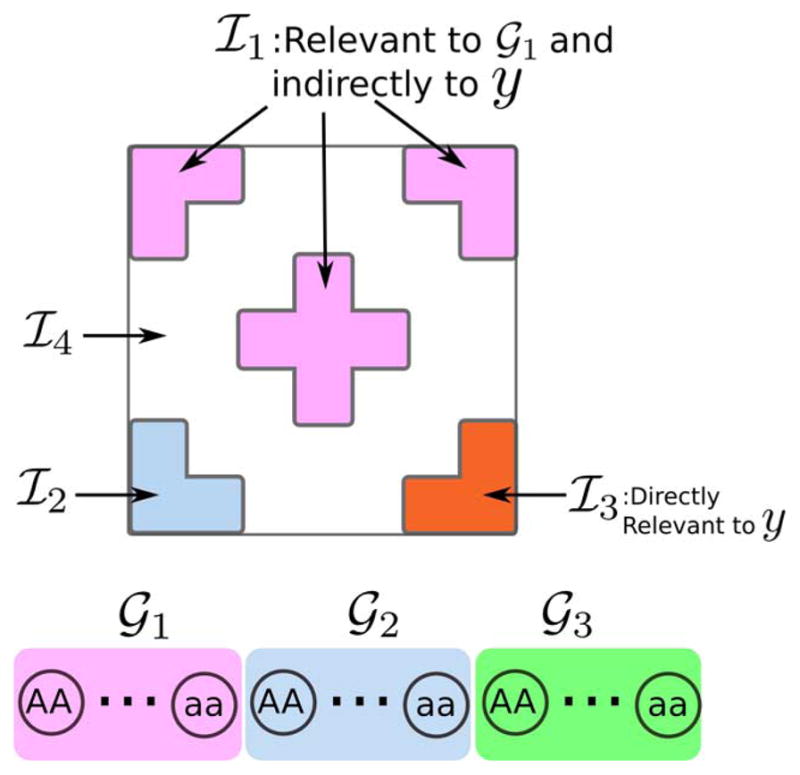
Summary of the simulation setup. For both healthy subjects and diagnosed patients we split the genome into three regions, and the image into six regions of four types.

We use the synthetic data to evaluate detection of causative SNPs with our method. As a first baseline method, we perform the univariate Bonferroni corrected t-test directly between SNPs and disease labels, omitting images. As a second baseline, which we refer to as supervised sRRR, we perform univariate voxel filtering using disease label, followed by the sRRR multivariate regression between the surviving voxels and the genetic variants to recover relevant SNPs [12]. We compare the methods in different image noise regimes by varying the variance ${\sigma }_{\text{noise}}^2$ in (16)– (17), and run 20 different independent simulations for each noise regime. We have also applied CCA, which can be viewed as sRRR but without sparsity regularization.

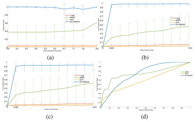
Fig. 4 reports the performance of all four methods for an odds ratio of 1.125. To illustrate the behavior of the methods for different false positive rates, we report the receiver operating characteristic at two different noise levels. In supervised sRRR, we observe that using a standard univariate filtering p-value cutoff of 5% eliminates too many image regions and does not successfully allow for detection of genetic variants, leading to poor performance. We increased the success rate of sRRR by keeping the top 40% of regions sorted by their p-values. We found that sRRR results were robust when varying this parameter in a range around this larger percentage of regions to be included in the method. To set the detection thresholds, we fix the false positive rate to 1%. We observe similar behavior for a broad range of low false positive rates (not shown). We focus our experiments on low false positive rates because at higher rates false detections become comparable with, and ultimately overwhelm true detections, since there are so few relevant variants. We find that for a given false positive rate, our algorithm detects significantly more disease causative SNPs in 𝒢₁ than the baseline algorithms, and has lower standard deviation than the supervised sRRR pipeline. The results of the CCA is consistently inferior with respect to sRRR. Given that sRRR can be viewed as CCA with sparsity constraints, this results emphasizes the importance of the sparsity regularization. The direct univariate t-tests only detect SNPs that have a very strong independent association with the disease label.

Fig. 4.

Summary of the results on simulated data. (a) Detection rates for our algorithm (blue), the supervised sRRR (green), CCA (orange), and genetic t-test (red) as a function of image noise for causative SNPs 𝒢₁ in at a false positive rate of 1%. (b,c) ROC curves for low ( ${\sigma }_{\text{noise}}^2=0.06$) and high ( ${\sigma }_{\text{noise}}^2=1.7$) noise levels respectively, up to the selected false positive threshold of 1%. The green shows the results of sRRR where any variant that has non-zero weight is considered a hit, and we vary the sparsity parameters. (d) ROC curve for the detection of relevant imaging regions for low ( ${\sigma }_{\text{noise}}^2=0.06$) noise level.

As more noise is added to the image, a two-step method starts to miss relevant regions across the image, which consequently degrades its detection rate on the genetic side. Our approach exploits other sources of information to compute the posterior probability of relevance. Namely, the p(b|𝒟) has two terms. The second term in (10) summarizes the contribution of the genetic data which helps to compensate for the “image noise”. In addition, genetics-to-image part of our model employs a powerful approach based on spike-and-slab prior. One can view spike-and-slab prior as a mixture of ℓ₀ and ℓ₂ regularization. This experiment shows that such regularization tends to perform better than ℓ₁ used in the sRRR approach. Better regularization and richer model explain the increased robustness of our approach compared to the “two-step” method.

V. Alzheimer’s Disease Data

A. Data and Preliminary Evidence

Before applying our method to real data, we familiarize the reader with the data by demonstrating evidence of the association between the clinical diagnosis y, image data X, and genotype G using a baseline approach.

We used clinical data from the ADNI study without focusing on a specific sub-group. ADNI is a large-scale study; the details on the study participants can be found elsewhere. The cohort includes 179 Alzheimer’s patients (AD) and 198 healthy subjects (healthy) to the total of 377 subjects. We employed FreeSurfer image analysis suite³ to process the MRI scans and produce segmentations and volume measurements for an array of regions (cortical and sub-cortical) that cover the entire brain. For details of these regions, please refer to Cortical ROIs⁴, Desikan ROIs⁵ in the FreeSurfer documentation. The technical details of these procedures are described in [29]–[32], and [33].

To extract genetic variants, the standard quality control was applied to remove rare genetic variants or variants violating the Hardy-Weinberg Principle [28]. To reduce the number of SNPs considered by the algorithm, we removed SNPs that are unlikely to be associated with AD. We first imputed our genotype data to the 1000 Genomes panel using MaCH [34], then kept only SNPs whose p-value (as measured by a large-scale meta-analysis of AD [35]) was below a liberal threshold (10⁻³), yielding 15,788 SNPs.

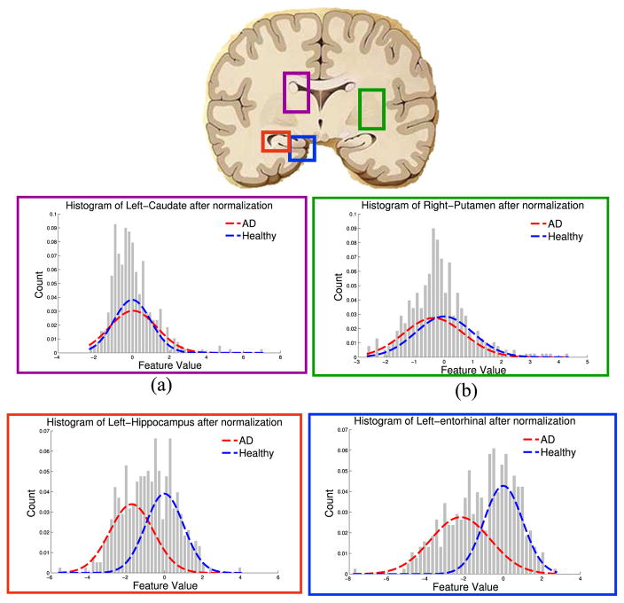
Fig. 5 reports histograms of image features in four representative brain regions for the two cohorts of healthy and AD subjects. Two of these regions are highly relevant to the disease (entorhinal cortex and hippocampus [36]) while the other two have been less reported (putamen [37] and caudate) in the context of Alzheimer’s disease. While the distribution of the cortical thickness in the left entorhinal cortex is strongly segregated across two cohorts, the right putamen and the left caudate volumes show weak or almost no statistical difference between the two populations. The entorhinal cortex is an important brain region responsible for declarative memories and memory consolidation and is implicated in early Alzheimer’s disease [38].

Fig. 5.

Distribution of the imaging features for four different regions of the brain are shown. None or very weak differences can be seen between the groups for caudate and putamen while there are very strong differences in the volume of the left hippocampus and the average thickness of the entorhinal cortex.

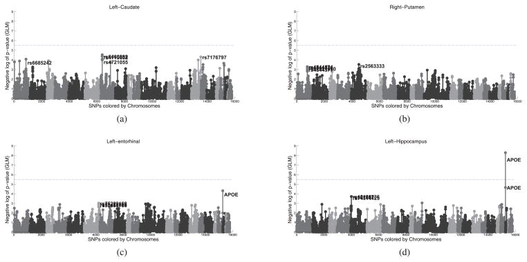
To experiment with a classical baseline Genome-Wide Association (GWAS) methods, we fit several Generalized Linear Models (GLM) using the genotype G as the design matrix. In Fig. 6, we used the image features from the four brain regions in Fig. 5 as the response variable to the GLM. The Manhattan plot in Fig. 6 shows −log₁₀ p-value for the genetic loci tested; the different shades of gray indicate different chromosomes. Despite the strong separation between healthy and AD in the left entorhinal cortex, no SNP passes the Bonferroni-corrected significance threshold. Nevertheless there is an indication for APOE variants. APOE is the only SNP that passes the significance level after the Bonferroni correction when the volume of the left hippocampus (Fig. 6(d)) or clinical diagnosis y (not shown) are used as the response variables. Fig. 6 therefore illustrates the limitation of classical GWAS.

Fig. 6.

Manhattan plots using different response variables in the GLM (a) volume of the left caudate (b) the volume of the right putamen (c) average cortical thickness of the left entorhinal cortex, and (d) volume of the left hippocampus. The x-axis lists the SNPs and the shades indicate different chromosomes. The y-axis reports the negative log₁₀ of the p-value. The vertical line denotes the statistical significance level (0.05) after Bonferroni correction. Only APOE variants pass significance level, but only for the volume of the left hippocampus. In spite of a clear distinction between distributions of healthy and AD for the left entorhinal cortex (Fig. 5), no SNP passes the significance level when using the average thickness of the left entorhinal cortex as a response variable.

B. Posterior Relevance of Brain Regions and SNPs

We applied our inference algorithm on the subset of the ADNI dataset described above. The algorithm shown integrates out the hyper-parameters through importance sampling. Only a range of hyper-parameters should be provided to the outer loop of algorithm, which translates to a weakly informative prior for the hyper-parameters. We choose the range for the hyper-parameters as follows:

σ₀ is the variance of the residual noise for the imaging features after they are explained by a subset of the genotype. For σ₀, we searched over [0.2,1]. Since the imaging features are normalized to have unit variance, the variance of the residual is upper bounded by 1. We also do not expect the genetic variant to explain all the variance in the imaging feature, hence we expect a residual variance. It is common to impose a non-informative prior over σ₀ by assuming the inverse-gamma distribution for σ₀ and setting its shape parameter to a small quantity (here 0.05, see Fig. 1(c) in the Supplementary Materials).

For the variance of effect of individual SNPs σ_ω, we searched over [0.025,0.4]. We do not expect a large contribution by a single SNP, but small contributions by several SNPs are possible. For this reason, the interval spans a small range. Notice that the variance of the residual, σ₀, is at most 1. In Section II-F, we explained that the proportion of variance explained (PVE) can be used to impose a prior over σ_ω as suggested in [17] (see Fig. 1(b) in Supplementary Material).

To investigate the prior probability α of any SNP to be relevant, the range of log₁₀ α is set to [−5, −3]. For 15,788 SNPs, this is equivalent of selecting 0.1 to 16 SNPs as relevant to the endophenotype a priori. Two positive shape parameters of the beta distribution are set to 1.02 and 1 respectively which imposes almost uniform prior for the selected range of α (Fig. 1(a) in the Supplementary Materials).

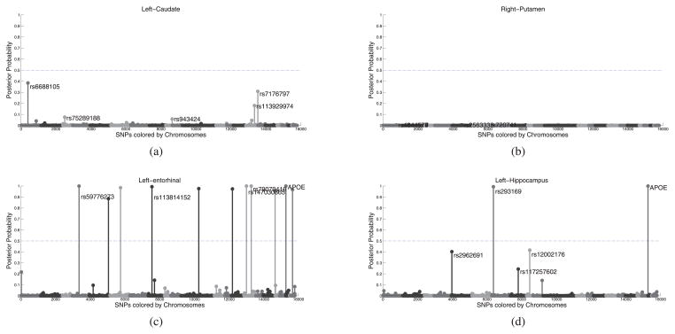
The posterior probability of the relevant SNPs (i.e., p(a_m|𝒟)) is reported in Fig. 7 for the brain regions examined in Figs. 5 and 6. The results of both approaches, i.e., the proposed model and the classical approach of univariate tests, are relatively consistent. The least informative regions such as the caudate and putamen are assigned no SNPs by either methods. The hippocampus, which is known to be correlated with AD, is associated with a variant in APOE, a genetic marker known to be associated with Alzheimer’s disease. For areas such as the entorhinal cortex, which is affected by AD [38], the classical method shows suggestive association for a variant in APOE, while for our method, APOE as well as a few others, pass the significance level.

Fig. 7.

Posterior relevance of the SNPs with respect to (a) volume of the left caudate, (b) right putamen, (c) average thickness of the left entorhinal cortex, and (d) volume of the left hippocampus, respectively. Compared to Fig. 6. The horizontal line indicates p = 0.5.

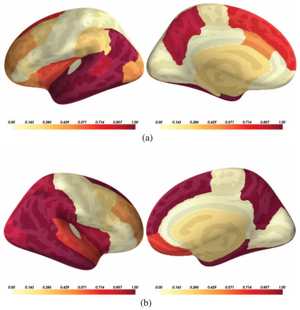
Interestingly, by computing the posterior relevance of brain regions p(b_m = 1|𝒟), we can go beyond the known regions of the brain affected by AD. Fig. 9 reports the posterior probability of brain regions being relevant jointly for the genotype and the diagnosis. Fig. 9(a) and (b) show two hemispheres of the brain on medial and lateral views; the color indicates the posterior probability. Fig. 8 represents the same results via a bar-plot. The y-axis is p(b_m = 1|𝒟). We sorted the regions according to the ranking produced by a classical correlation criterion (with respect to y). We observe that the classical statistical method and the results based on our model are largely consistent but our method assigns high posterior relevance to some regions that are viewed less important according to the classical test.

Fig. 9.

Posterior probability of the relevant regions (i.e., p(b|𝒟)) for (a) left and (b) right hemispheres of the brain. Left and right figures in each row represent lateral and medial views respectively. The color indicates the value of the posterior probability, the hotter color, the higher the posterior. (a) Left. (b) Right.

Fig. 8.

The barplot of the posterior relevance for all 94 brain regions (y-axis). The regions are ordered according to the ranking produced by the two sample T-test with respect to y: We conducted a t-test to examine the difference between cases and controls for each one of these measurements and ranked them based on the t-test result.

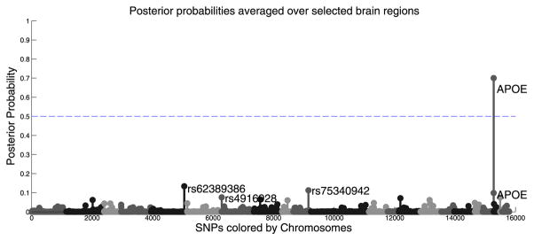
We emphasize that our method does not pool the genetic risk across ROIs. One can get a single set of posterior probability for all SNPs by summarizing overall association (see the Fig. 10). This can be simply done by multiplying the posterior probability of the regions by the posterior probability of SNPs and summing over all brain regions that pass the 1/2 threshold. Interestingly, the results are consistent with pair-wise association between genotype and diagnosis and only APOE passes the detection threshold. However, this does not mean that APOE is the only significant marker but it says that APOE is the one that almost all regions agree on due to its large effect. There is no reason to believe that genetic variants affect all regions equally. In fact, variations across locations is an interesting and worthy topic for further study.

Fig. 10.

Averaging regional posterior values across the selected brain regions. Only APOE is significant which means APOE is the one marker that many regions are consistently affected by.

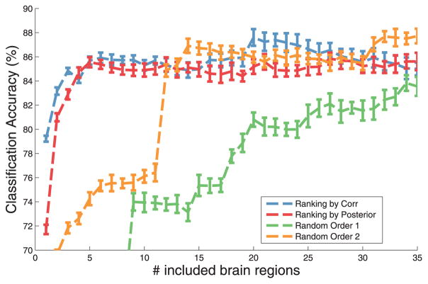
In Fig. 11, we investigate if regions with high posterior relevance are related to AD, by examinining the importance of the features for prediction of the diagnosis. The x-axis is the number of features incrementally included in a linear classifier and y-axis is the cross-validation accuracy of the prediction of the diagnosis. Different curves denote rankings of the features according to the posterior values, correlation with diagnosis y, or random permutations (two instances). As we add more features, the accuracy of prediction increases. Our method closely follows the correlation ranking which indicates that the regions with high posterior values are closely related to the disease while the random rankings (i.e., permutations) lag behind and need to include many features to finally match the accuracy of the informed methods. It is worth noting that correlation with diagnosis y only accounts for the diagnosis while the posterior values incorporate both genetic indicators and diagnosis simultaneously.

Fig. 11.

Accuracy of the prediction of the disease for different number of input features ranked by correlation with disease diagnosis (blue), posterior produced by our method (red), and random ordering (orange and green). While our method and the correlation method jump quickly, it takes many more features for random ordering to match the accuracy of the informed methods.

C. Sensitivity Analysis

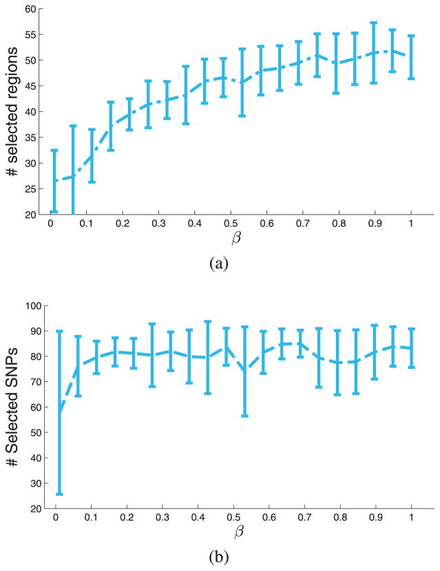
In Section II-F, we described the prior probabilities over variables α, ${\sigma }_0^2$, and ${\sigma }_{\omega }^2$. The hyper-parameters of those variables are integrated out using importance sampling by gridding the hyper-parameters over the their corresponding intervals (see Supplementary Material). In Section V-B, we explained how to choose these intervals depending on the meaning of the random variables and the data. In this section, we explore the sensitivity of the results with respect to the only remaining parameter β that specifies a prior number of relevant image regions. We change β from 1/94 to 94/94. For each value of β, we run the inference algorithm 20 times. Fig. 12 reports the results.

Fig. 12.

(a) The number of selected image regions for different values of the prior β (i.e., Σ_m [p(b_m|𝒟) > 1/2]). (b) The total number of selected SNPs (i.e., Σ_s [min_m [P (a_sm|𝒟)] > 1/2]).

We examine the number of brain regions with posterior probability higher than 0.5 computed as Σ_m [p(b_m|𝒟) > 1/2]. Although this quantity increases with β, the model never chooses all regions, suggesting that some regions are not relevant regardless of the prior.

We also report the total number of selected SNPs (Σ_s [p(a_m|𝒟) > 1/2]) for different values of β. The curve plateaus at 80 quickly, suggesting that SNP selection is not very sensitive to the value of the prior. We can choose β in a reasonable range (depending on the application) with the least variance in Fig. 12(b). In all experiments of Section V-B, we set β = 10/94 which lies in the plateaus region in Fig. 12 and has low variance.

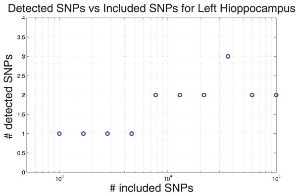
To study the behavior of the method empirically, we applied the model to the volume of left hippocampus as an intermediate phenotype (Fig. 13). It shows that the number of detected SNP saturates as we include more SNPs in the model.

Fig. 13.

The x-axis shows the number of SNPs included into the model, y-axis shows the number of selected SNPs when the volume of left hippocampus is used as the response variable in a Spike-and-Slab model.

For 10⁵ SNPs our algorithm takes about 24 hours to run. Other than computational cost, the problem with large number of SNPs is that the method starts missing APOE as the most important variant. We hypothesize it is due to small sample size and highly non-convex landscape of the objective function. Improving the stability of the method is an interesting direction of future research.

D. Biological Pathway Analysis

To investigate the molecular mechanisms through which these SNPs may be impacting brain morphology and AD phenotype, we mapped the 83 SNPs that were likely to target at least one brain region to the nearest genes on the genome through the following procedure. We systematically filtered the 83 SNPs for dbSNP IDs and pruned the 83 SNPs based on linkage disequilibrium down to 77 SNPs. The pruning algorithm looks at all possible pairs of the 83 SNPs (for which their Pearson correlation is at least 0.2 from the 1000 Genomes Phase One European data [39]) and marks the SNP with lower rank for removal from the list. To determine SNP ranks, the algorithm first orders all SNPs by the number of brain regions in which their posterior is at least 0.5, then breaks ties based on the maximum posterior achieved in any brain region. We then mapped all SNPs to their nearest up and downstream protein-coding gene based on GENCODE version 10 annotations [40]. From the resulting list of 154 genes, we used Fisher’s exact test to measure enrichment of our AD SNPs against 1024 known human pathways (whose size ranged from 5 to 300 genes inclusive) from the June 2011 release of the Pathway Commons database [41] (See Table II in the Supplementary File for the list of SNPs and genes).

We found those nearest genes are significantly enriched in two biological pathways (α < 0.05, Benjamini-Hochberg FDR), the Netrin signaling and the α4β1 integrin pathways. Four genes proximal to our SNPs were direct interactors of the Netrin-1 protein complex (PITPNA, TRIO, MAP1B and DAPK1) within the Netrin signaling pathway. Netrin is a highly conserved protein involved in axon development, and is associated with negative regulation of amyloid-β production in the brains of Alzheimer’s mice models [42], [43]. The amyloid-β peptide is the main component of amyloid plaques that is the hallmark of Alzheimer’s Disease.

Four additional genes either formed direct complexes with, or directly interacted with, α4β1 integrin, as part of the α4β1 integrin signaling pathway. α4β1 mediates permeation of blood barrier by leukocyte immune cells [44] and plays an important role both biologically and as a drug target in immune related diseases such as multiple sclerosis [45]. α4β1 is not reported to be related to the Alzheimer’s disease but it is consistent with recent work that suggests genetic variants associated with Alzheimer’s disease target regulatory elements in leukocytes and other immune cells rather than brain cells [46], [47].

We also applied a separate regression and computed the residual to remove the effect of covariates (age, handedness, gender, and education). Then, we applied the algorithm on the residual and noticed that the enrichment is not statistically significant. This suggests that the enrichment signal is weak and to correct for the effect of the covariates, they should be incorporated into (2).

VI. Discussion

In this paper, we propose a Bayesian method to identify indirect genetic associations with a diagnosis using image phenotype. Our model integrates two components: 1) selection of intermediate imaging phenotypes influenced by genetic markers and relevant to the disease and, 2) quantification of genetic associations with the disease mediated by the imaging variables. A classical strategy is to perform these two steps separately. First, an association analysis between imaging variables and disease phenotype is carried out. This step identifies imaging variables relevant to the disease status. Then, the associations between the relevant imaging markers and genotype data are probed. By performing these two tasks jointly, we avoid choosing an arbitrary threshold for feature selection.

We note that the model does not pool the genetic risk across ROIs. SNPs associated with complex diseases tend to act on cell type specific regulatory elements [48], suggesting that individual SNPs may be targeting specific cell types, and therefore brain regions. Furthermore, brain regions exhibit unique gene expression signatures [49] and epigenetic/regulatory signatures (Roadmap Epigenomics Consortium [50]), and therefore would be expected to use different sets of pathways to perform normal function.

Indeed, one can get a single set of posterior probabilities for all SNPs summarizing overall association (Fig. 10). This can be simply achieved by multiplying the posterior probability of the regions by the posterior probability of SNPs and summing over all brain regions that pass a threshold of 0.5. Interestingly, the result is consistent with pair-wise associations between the genotype and diagnosis and only APOE passes the 0.5 threshold. However, this does not mean that only APOE is the significant marker but rather that APOE is the marker that almost all regions are consistently affected by.

In this paper, we assumed that genetic variants related to the disease encode variations measurable by imaging data. This assumption has some limitations. For example, if the genetic variants related to the disease do not manifest themselves on the imaging data, our method cannot detect it. Another limitations is for the genetic variants that have both normal and disease-related effects; such case is not identifiable by our model but to the best of our knowledge it is not identifiable by other approaches as well. These challenges provide fruitful directions for future work.

In this paper, we assume that genetic variants G have indirect associations to the disease label y. In other words, we assume that all relevant genetic associations are already captured by the image features. It is conceivable that some of the variants have a direct association, i.e., their impact is not captured by the imaging features. It is possible to extend the graphical model to incorporate such effects by introducing a direct connection from G to y. Such a change in the graphical model renders the inference procedure more complex.

Our model ranks brain regions based on the amount of variance of imaging features explained by the genotype. The ranking of the regions gets updated according to the relevance of the brain regions to the diagnosis. The proposed procedure approximates two posterior probabilities, p(b|𝒟) and p(a_m|𝒟), denoting the relevance of image regions for the disease and of the genotype related to those regions, respectively.

There are two major reasons for using region-based image features: statistical and computational. Statistically, aggregate measures such as region-based image features provide more robust estimators at the expense of a coarser resolution on delineating affected brain regions. From the computational point of view, reducing the number of brain regions (fewer b_m) reduces the computational cost of Algorithm 1 (see supplementary file). Every iteration of Algorithm 1 entails solving a linear system with O(M) (M is the number of brain regions) variables.

We use the language of directed graphical models to formalize our assumptions. We use Gaussian Process (GP) to model the diagnosis. The GP framework is flexible, enabling a range of functions (i.e., f in the graphical model) to be used by simply changing the kernel function. To extend the method to regression (i.e., continuous y), one needs to modify the likelihood function in (1) and to modify a noise model. Interestingly, for the regression case with the Gaussian noise, the marginal likelihood ℙ(y|b, 𝒟) has a closed-form solution and one does not need to resort to Expectation Propagation (EP) for approximation. Many noise models were investigated in [16], deriving efficient algorithms to approximate the marginal likelihood for many members of the exponential family.

The image-to-disease phenotype part of the model can be extended such that the diagnosis variable y encodes finer levels of diagnosis. For example, we can replace the logistic regression likelihood with the ordinal logistic likelihood [51] to encode discrete and ordered observations about the disease (Healthy (j = 0) < MCI (j = 1) < AD (j = 2)):

$$p(y\le j\mid \mathbf{x},\mathit{\nu },{\theta }_1,{\theta }_2,{\theta }_3)=\frac{1}{1+exp({\mathbf{x}}^T\mathit{\nu }-{\theta }_j)},$$ (18)

where ν and the θ₁ < θ₂ < θ₃ are the parameters of the ordinal logistic regression and j encodes the ordinal stage of the Alzheimer’s disease.

We model the null distribution of the image regions with a Gaussian distribution. This assumption can be easily modified by replacing the Gaussian distribution with any other distribution depending on the application. The noise model for the alternative hypothesis (i.e., b_m = 1) can also be modified. The challenge is to compute the marginal likelihood efficiently (i.e., ℙ(X_:m|b_m = 1; G)). We approximate this value by the lower bound provided by the variational approximation. Our current implementation supports the Gaussian noise assumption for imaging features X_:m. We leave the relaxation of this assumption to future work. We believe, at least for the most common members of the exponential family, slight modification to the variational algorithm should be possible.

The hidden random variable b encodes the relevant regions. Therefore, the kernel depends on b. For example the linear kernel between two samples x_i and x_j should be defined as

$$k_{\mathbf{b}}(\mathbf{x},{\mathbf{x}}^{\prime })={(\mathbf{xb})}^T({\mathbf{x}}^{\prime }\mathbf{b}).$$

Note that b appears in the definition of the kernel. We chose the linear kernel because of its simplicity. Although it is possible to use a complex kernel together with a regularization, we avoided it because of two reasons. First, this would introduce extra parameter (e.g., kernel width in case of Radial Basis Function). Second, the value of such parameter would depend on an unknown parameter b. In the case of RBF, kernel width should scale with the dimensionality of the input vector. In our case, the input vector consists of the relevant regions selected by the indicator variable b. Note that this is not the case in the classical kernel-based approaches where the prediction is the only goal but not features selection. Previously demonstrated methods for feature selection using kernel machines [52] lack a probabilistic model required by our approach. Further extension of our model to those cases is possible but beyond the scope of this paper.

In addition to minor modifications to the structure of the graphical model compared to our previous work [15], there are several major innovations introduced in this paper. First, in the image-to-phenotype part of the model, we employed the Gaussian process to model the prediction function. This modification enables us to model the complex relationship between image and clinical phenotypes. In this paper, we focused on the linear kernel to avoid over-fitting but in the presence of more samples a more sophisticated prediction function can be reliably learned. The second major contribution is in the inference algorithm. It is more stable and scalable than our earlier inference method in [15]. The flexibility of the inference algorithm enabled us to go beyond conditionally independent intermediate phenotypes. For example, we are currently pursuing the case where intermediate phenotypes are highly correlated. In this case, two intermediate phenotypes (e.g., two brain regions) which are highly correlated should be viewed as approximately one phenotype. One can account for this phenomenon by modifying the prior probability of p(b) of the selector variable b. As long as we can sample efficiently from p(b), the inference algorithm is computationally tractable.

Two key quantities that determine the computational complexity of the inference algorithm are the marginal likelihoods p(y|b, 𝒟) and p(X_:m|b_m = 1; G). If no value is missing from the intermediate phenotypes, p(X_:m|b_m = 1; G)can be computed in parallel and stored p(y|b, 𝒟). needs to be computed for every draw of b. We use expectation propagation (EP), which is very fast, particularly for the small sample size prevalent in imaging genetic applications (cf. [16, Section 3.6]).

As suggested in [17], fast computation of the variational lower bound enables us to perform importance sampling and to integrate out all hyper-parameters other than the image feature selection prior β. Since we have few hyper-parameters, we only need to specify a reasonable range for each hyper-parameter. This approach also enables us to define a weakly-informed prior over the hyper-parameters. Depending on the meaning of each hyper-parameter, we defined a range that is reasonable for the application. We provide an example in Section V-B on how to choose the intervals. In Section V-C, we show that the total number of SNPs detected by the inference is not very sensitive to the specific value of β.

In Section V-B, we compared the associated SNPs to the relevant brain regions using the p-values and the posterior probabilities. Although the p-value and the posterior probability do not have the same meaning, their suggestions about the data are relatively consistent. We showed in Figs. 6 and 7 that the less important regions such as the putamen and the caudate do not exhibit associations in either method. Both techniques agree on the SNPs associated with left hippocampus. For the left entorhinal cortex, our method detects a few more SNPs in addition to the APOE variants. Furthermore, our method suggests areas to investigate further. Fig. 8 showed that posterior relevance values are mostly consistent with a classical ranking results but the proposed method does not require pre-selection and considers all available data.

The results reported for the univariate approach used Bonferroni correction which is a common practice in genetic association. Bonferroni correction is a conservative multiple hypothesis correction approach in comparison to controlling false discovery. In fact, one can further analyze the results reported by our approach and apply the hypothesis testing using the image features of the detected brain regions as a response variable of a GLM and correct the results with a method of choice. Our focus has been on how to incorporate information from different sources, here diagnosis, imaging and genetics data, into one model, and not on addressing multiple hypothesis correction approaches.

VII. Conclusion

We proposed and demonstrated a unified framework for identifying genetic variants and image-based features associated with the disease. We captured the associations between imaging and disease phenotype simultaneously with the correlation from genetic variants and image features in a probabilistic model. Our model also produces spatial distribution of the genetic associations. We derive an efficient and scalable algorithm based on variational inference. We did not assume any interaction between intermediate phenotypes (i.e., imaging features) but our method can be extended easily to handle such interactions. We demonstrated the benefit of simultaneously performing these two tasks (i.e., finding relevant genetic and brain regions) in simulations and in a context of a real clinical study of the Alzheimer’s disease.

References

- 1.Hoggart CJ, Whittaker JC, De Iorio M, Balding DJ. Simultaneous analysis of all SNPs in genome-wide and re-sequencing association studies. PLoS Genet. 2008;4(7):e1000130. doi: 10.1371/journal.pgen.1000130. [DOI] [PMC free article] [PubMed] [Google Scholar]
- 2.Lvovs D, et al. A polygenic approach to the study of polygenic diseases. Acta Naturae. 2012;4(3):59. [PMC free article] [PubMed] [Google Scholar]
- 3.Meyer-Lindenberg A, Weinberger DR. Intermediate phenotypes and genetic mechanisms of psychiatric disorders. Nature Rev Neurosci. 2006;7(10):818–827. doi: 10.1038/nrn1993. [DOI] [PubMed] [Google Scholar]
- 4.Glahn DC, Thompson PM, Blangero J. Neuroimaging endophenotypes: Strategies for finding genes influencing brain structure and function. Human Brain Mapp. 2007;28(6):488–501. doi: 10.1002/hbm.20401. [DOI] [PMC free article] [PubMed] [Google Scholar]
- 5.Batmanghelich NK, et al. Generative-discriminative basis learning for medical imaging. IEEE Trans Med Imag. 2012 Jan;31(1):51–69. doi: 10.1109/TMI.2011.2162961. [DOI] [PMC free article] [PubMed] [Google Scholar]
- 6.Sabuncu M, et al. The relevance voxel machine (RVoxM): A Bayesian method for image-based prediction. In: Peters T, Fichtinger G, Martel A, editors. MICCAI 2011. Heidelberg; Germany: 2011. pp. 99–106. LNCS. [DOI] [PMC free article] [PubMed] [Google Scholar]
- 7.Filippini N, et al. Anatomically-distinct genetic associations of APOE epsilon4 allele load with regional cortical atrophy in Alzheimer’s disease. Neuroimage. 2009 Feb;44(3):724–728. doi: 10.1016/j.neuroimage.2008.10.003. [DOI] [PubMed] [Google Scholar]
- 8.Potkin S, et al. A genome-wide association study of schizophrenia using brain activation as a quantitative phenotype. Schizophr Bull. 2009 Jan;35(1):96–108. doi: 10.1093/schbul/sbn155. [DOI] [PMC free article] [PubMed] [Google Scholar]
- 9.Sabuncu MR, et al. The association between a polygenic alzheimer score and cortical thickness in clinically normal subjects. Cerebral Cortex. 2012;22(11):2653–2661. doi: 10.1093/cercor/bhr348. [DOI] [PMC free article] [PubMed] [Google Scholar]
- 10.Stein J, et al. Voxelwise genome-wide association study (vGWAS) Neuroimage. 2010 Nov;53(3):1160–1174. doi: 10.1016/j.neuroimage.2010.02.032. [DOI] [PMC free article] [PubMed] [Google Scholar]
- 11.Le Floch E, et al. Significant correlation between a set of genetic polymorphisms and a functional brain network revealed by feature selection and sparse Partial Least Squares. Neuroimage. 2012 Oct;63(1):11–24. doi: 10.1016/j.neuroimage.2012.06.061. [DOI] [PubMed] [Google Scholar]
- 12.Vounou M, et al. Discovering genetic associations with high-dimensional neuroimaging phenotypes: A sparse reduced-rank regression approach. Neuroimage. 2010 Nov;53(3):1147–1159. doi: 10.1016/j.neuroimage.2010.07.002. [DOI] [PMC free article] [PubMed] [Google Scholar]
- 13.Vounou M, et al. Sparse reduced-rank regression detects genetic associations with voxel-wise longitudinal phenotypes in Alzheimer’s disease. Neuroimage. 2012 Mar;60(1):700–716. doi: 10.1016/j.neuroimage.2011.12.029. [DOI] [PMC free article] [PubMed] [Google Scholar]
- 14.Mueller S, et al. The alzheimer’s disease neuroimaging initiative. Neuroimag Clin N Am. 2005;15(4):869. doi: 10.1016/j.nic.2005.09.008. [DOI] [PMC free article] [PubMed] [Google Scholar]
- 15.Batmanghelich NK, et al. Information Processing in Medical Imaging. New York: Springer; 2013. Joint modeling of imaging and genetics; pp. 766–777. [DOI] [PMC free article] [PubMed] [Google Scholar]
- 16.Rasmussen CE, Williams CKI. Gaussian Processes for Machine Learning. Cambridge, MA: MIT Press; 2006. [Google Scholar]
- 17.Carbonetto P, Stephens M. Scalable variational inference for Bayesian variable selection in regression, and its accuracy in genetic association studies. Bayesian Anal. 2012;7:73–108. [Google Scholar]
- 18.Mitchell TJ, Beauchamp JJ. Bayesian variable selection in linear regression. J Am Stat Assoc. 1988;83(404):1023–1032. [Google Scholar]
- 19.Gelman A, et al. Prior distributions for variance parameters in hierarchical models (comment on article by Browne and Draper) Bayesian Anal. 2006;1(3):515–534. [Google Scholar]
- 20.Jeffreys H. An invariant form for the prior probability in estimation problems. Proc R Soc London, Ser A, Math Phys Sci. 1946;186:453–461. 1007. doi: 10.1098/rspa.1946.0056. [DOI] [PubMed] [Google Scholar]
- 21.Guan Y, et al. Bayesian variable selection regression for genome-wide association studies and other large-scale problems. Ann Appl Stat. 2011;5(3):1780–1815. [Google Scholar]
- 22.Koller D, Friedman N. Probabilistic Graphical Models: Principles and Techniques. Cambridge, MA: MIT Press; 2009. [Google Scholar]
- 23.Bishop CM. Pattern Recognition and Machine Learning. New York: Springer; 2006. [Google Scholar]
- 24.Beal M, Ghahramani Z. The variational Bayesian EM algorithm for incomplete data: With application to scoring graphical model structures. Bayesian Stat. 2003;7:1–10. [Google Scholar]
- 25.Salimans T, et al. Fixed-form variational posterior approximation through stochastic linear regression. Bayesian Anal. 2013;8(4):837–882. [Google Scholar]
- 26.Honkela A, et al. Approximate Riemannian conjugate gradient learning for fixed-form variational Bayes. J Mach Learn Res. 2010;9999:3235–3268. [Google Scholar]
- 27.Nemirovski A, et al. Robust stochastic approximation approach to stochastic programming. SIAM J Optimizat. 2009;19(4):1574–1609. [Google Scholar]
- 28.Purcell S, et al. PLINK: A tool set for whole-genome association and population-based linkage analyses. Am J Hum Genet. 2007 Sep;81(3):559–575. doi: 10.1086/519795. [DOI] [PMC free article] [PubMed] [Google Scholar]
- 29.Fischl B, et al. Automatically parcellating the human cerebral cortex. Cerebral Cortex. 2004;14(1):11–22. doi: 10.1093/cercor/bhg087. [DOI] [PubMed] [Google Scholar]
- 30.Dale AM, Fischl B, Sereno MI. Cortical surface-based analysis: I. Segmentation and surface reconstruction. Neuroimage. 1999;9(2):179–194. doi: 10.1006/nimg.1998.0395. [DOI] [PubMed] [Google Scholar]
- 31.Fischl B, Sereno MI, Dale AM. Cortical surface-based analysis: II: Inflation, flattening, and a surface-based coordinate system. Neuroimage. 1999;9(2):195–207. doi: 10.1006/nimg.1998.0396. [DOI] [PubMed] [Google Scholar]
- 32.Fischl B, et al. Whole brain segmentation: Automated labeling of neuroanatomical structures in the human brain. Neuron. 2002;33(3):341–355. doi: 10.1016/s0896-6273(02)00569-x. [DOI] [PubMed] [Google Scholar]
- 33.Fischl B, Dale AM. Measuring the thickness of the human cerebral cortex from magnetic resonance images. Proc Nat Acad Sci. 2000;97:11 050–11 055. 20. doi: 10.1073/pnas.200033797. [DOI] [PMC free article] [PubMed] [Google Scholar]
- 34.Li Y, et al. MaCH: Using sequence and genotype data to estimate haplotypes and unobserved genotypes. Genetic Epidemiol. 2010;34(8):816–834. doi: 10.1002/gepi.20533. [DOI] [PMC free article] [PubMed] [Google Scholar]
- 35.Lambert J-C, et al. Meta-analysis of 74,046 individuals identifies 11 new susceptibility loci for Alzheimer’s disease. Nature Genetics. 2013 doi: 10.1038/ng.2802. [DOI] [PMC free article] [PubMed] [Google Scholar]
- 36.Whitehouse PJ, et al. Alzheimer’s disease and senile dementia: Loss of neurons in the basal forebrain. Science. 1982;215(4537):1237–1239. doi: 10.1126/science.7058341. [DOI] [PubMed] [Google Scholar]
- 37.De Jong L, et al. Strongly reduced volumes of putamen and thalamus in Alzheimer’s disease: An MRI study. Brain. 2008;131(12):3277–3285. doi: 10.1093/brain/awn278. [DOI] [PMC free article] [PubMed] [Google Scholar]
- 38.Khan UA, et al. Molecular drivers and cortical spread of lateral entorhinal cortex dysfunction in preclinical Alzheimer’s disease. Nature Neurosci. 2014;17(2):304–311. doi: 10.1038/nn.3606. [DOI] [PMC free article] [PubMed] [Google Scholar]
- 39.Consortium TGP. An integrated map of genetic variation from 1,092 human genomes. Nature. 2012 doi: 10.1038/nature11632. [DOI] [PMC free article] [PubMed] [Google Scholar]
- 40.Harrow J, et al. GENCODE: The reference human genome annotation for the encode project. Genome Res. 2012 doi: 10.1101/gr.135350.111. [DOI] [PMC free article] [PubMed] [Google Scholar]
- 41.Cerami E, et al. Pathway commons, a web resource for biological pathway data. Nucleic Acids Res. 2011 doi: 10.1093/nar/gkq1039. [DOI] [PMC free article] [PubMed] [Google Scholar]
- 42.Rama N, et al. Amyloid precursor protein regulates netrin-1-mediated commissural axon outgrowth. J Biol Chem. 2012;287(35):300014–30023. doi: 10.1074/jbc.M111.324780. [DOI] [PMC free article] [PubMed] [Google Scholar]
- 43.Lourenco F, et al. Netrin-1 interacts with amyloid precursor protein and regulates amyloid-β production. Cell Death Differentiation. 2009 doi: 10.1038/cdd.2008.191. [DOI] [PMC free article] [PubMed] [Google Scholar]
- 44.Takeshita Y, Ransohoff R. Inflammatory cell trafficking across the blood–brain barrier: Chemokine regulation and in vitro models. Immunological Rev. 2012 doi: 10.1111/j.1600-065X.2012.01127.x. [DOI] [PMC free article] [PubMed] [Google Scholar]
- 45.Buzzard K, et al. What do effective treatments for multiple sclerosis tell us about the molecular mechanisms involved in pathogenesis? Int J Molecular Sci. 2012;13(10):12665–12709. doi: 10.3390/ijms131012665. [DOI] [PMC free article] [PubMed] [Google Scholar]
- 46.Gjoneska E, et al. Conserved epigenomic signals in mice and humans reveal immune basis of Alzheimer’s disease. Nature. 2015;518(7539):365–369. doi: 10.1038/nature14252. [DOI] [PMC free article] [PubMed] [Google Scholar]
- 47.Raj T, et al. Polarization of the effects of autoimmune and neurodegenerative risk alleles in leukocytes. Science. 2014;344(6183):519–523. doi: 10.1126/science.1249547. [DOI] [PMC free article] [PubMed] [Google Scholar]
- 48.Maurano MT, et al. Systematic localization of common disease-associated variation in regulatory DNA. Science. 2012;337(6099):1190–1195. doi: 10.1126/science.1222794. [DOI] [PMC free article] [PubMed] [Google Scholar]
- 49.Hawrylycz MJ, et al. An anatomically comprehensive atlas of the adult human brain transcriptome. Nature. 2012;489(7416):391–399. doi: 10.1038/nature11405. [DOI] [PMC free article] [PubMed] [Google Scholar]
- 50.Kundaje A, et al. Integrative analysis of 111 reference human epigenomes. Nature. 2015;518(7539):317–330. doi: 10.1038/nature14248. [DOI] [PMC free article] [PubMed] [Google Scholar]
- 51.Liao TF. Interpreting probability models: Logit, probit, and other generalized linear models. New York: Sage; 1994. [Google Scholar]
- 52.Allen GI. Automatic feature selection via weighted kernels and regularization. J Comput Graph Stat. 2013;22(2):284–299. [Google Scholar]
Associated Data
This section collects any data citations, data availability statements, or supplementary materials included in this article.