Correlated variability modifies working memory fidelity in primate prefrontal neuronal ensembles

Significance

The working memory (WM)-related activity in the primate prefrontal cortex (PFC) is hypothesized to arise from the structure of the network in which the neurons are embedded. Recent studies have also shown that it is difficult to predict the properties of neuronal ensembles from the properties of individually examined neurons. By recording the activity of neuronal ensembles in the macaque PFC, we found evidence supporting the network origins of WM activity and discovered features of WM coding in neuronal ensembles that were inaccessible in prior single neuron studies. Most notably, we found that correlated firing rate variability between neurons (i.e., noise correlations) can improve WM coding and that neurons not selective for WM can improve WM coding when part of an ensemble.

Abstract

Neurons in the primate lateral prefrontal cortex (LPFC) encode working memory (WM) representations via sustained firing, a phenomenon hypothesized to arise from recurrent dynamics within ensembles of interconnected neurons. Here, we tested this hypothesis by using microelectrode arrays to examine spike count correlations (r_sc) in LPFC neuronal ensembles during a spatial WM task. We found a pattern of pairwise r_sc during WM maintenance indicative of stronger coupling between similarly tuned neurons and increased inhibition between dissimilarly tuned neurons. We then used a linear decoder to quantify the effects of the high-dimensional r_sc structure on information coding in the neuronal ensembles. We found that the r_sc structure could facilitate or impair coding, depending on the size of the ensemble and tuning properties of its constituent neurons. A simple optimization procedure demonstrated that near-maximum decoding performance could be achieved using a relatively small number of neurons. These WM-optimized subensembles were more signal correlation (r_signal)-diverse and anatomically dispersed than predicted by the statistics of the full recorded population of neurons, and they often contained neurons that were poorly WM-selective, yet enhanced coding fidelity by shaping the ensemble’s r_sc structure. We observed a pattern of r_sc between LPFC neurons indicative of recurrent dynamics as a mechanism for WM-related activity and that the r_sc structure can increase the fidelity of WM representations. Thus, WM coding in LPFC neuronal ensembles arises from a complex synergy between single neuron coding properties and multidimensional, ensemble-level phenomena.

To interact with a complex, dynamic environment, organisms must be capable of maintaining and manipulating information that is no longer available to their sensory systems. This capability, when applied transiently (i.e., for milliseconds to seconds), is referred to as working memory (WM) (1)—a hallmark of intelligence and a crucial component of goal-directed behavior (2). In 1949, Hebb postulated that sustained neuronal activity in the absence of stimulus input could serve as the neural substrate for WM (3). Fuster and Alexander later discovered neurons in the lateral prefrontal cortex (LPFC) of monkeys that exhibited sustained firing during WM tasks (4). Subsequent neurophysiological studies have corroborated that neuronal activity in the LPFC and other regions can represent WM for visual–mnemonic space (5–7), as well as nonspatial visual features (8–10).

Electrophysiological studies of spatial WM have traditionally relied on recording from one neutron or a few neurons simultaneously (10). However, the neuronal computations that underlie sophisticated behaviors such as WM require the coordinated activity of many neurons within and across brain networks (11). We currently lack a clear understanding of how single neuron coding properties scale to neuronal ensembles. Can the properties of an ensemble be predicted by aggregating the individually and independently measured properties of its constituent neurons? The answers to this question and related questions hinge on how ensembles are affected by phenomena that emerge from interactions between neurons.

The sustained activity presumed to underlie WM maintenance is thought to be achieved by increasing the strength of recurrent excitation and lateral inhibition between neurons within an ensemble (12–18). These dynamics should modify patterns of correlated firing between neurons in a manner dependent on differences in their tuning properties. Such a pattern can be quantitatively characterized by two measurements: The first is signal correlation (r_signal), the similarity of two neurons’ responses to a set of different stimuli or experimental conditions. The second is spike count (or noise) correlations (r_sc), the similarity in the variability of two neurons’ responses to the same stimulus or experimental condition (19).

Given a fixed ensemble of neurons (and thus a constant r_signal structure), changes in r_sc can have profound effects on information coding (19–24). For example, spatial attention improves neural coding in the visual cortex primarily by reducing r_sc (25–27). Another study reported that increased r_sc improved perceptual discrimination in macaque area S2 (28). These results are difficult to extend to WM coding in the LPFC. Furthermore, there are relatively few studies investigating r_sc in the LPFC (21, 27, 29–33); and only one of these studies directly examined the effects of r_sc on information coding (27). Prior results examining pairwise correlations are also difficult to extrapolate to larger neuronal ensembles, which have a complex, multidimensional r_sc structure that cannot be characterized by pairwise measurements alone (20). Currently it remains unknown whether and how r_sc structure modulates the fidelity of WM coding in LPFC neuronal ensembles.

We used microelectrode arrays (MEAs) to record from neuronal ensembles in the LPFC of two monkeys while they performed an oculomotor delayed-response task and assessed ensemble information content using a linear decoder. We found that r_sc varied as a function of r_signal during WM maintenance in a manner predicted by a recurrent excitation and lateral inhibition scheme. Using all simultaneously recorded neurons, the decoder could reliably predict which of 16 locations was being remembered. We also devised procedures to systematically investigate how WM coding varies across the “configuration space” of potential neuronal ensembles. Removing the r_sc structure could increase or decrease the information content of neuronal ensembles across the configuration space. However, the intrinsic r_sc structure improved WM coding in smaller neuronal subensembles of neurons optimized for WM representation. These optimized ensembles had a stereotyped r_signal distribution, with peaks at zero and extreme negative values, and spanned farther across the cortical surface than predicted by the statistics of the full population of recorded LPFC units. Finally, we observed individual units that did not encode WM in isolation (“nonselective” neurons) but that still contributed to WM coding when part of an ensemble by altering the r_sc structure.

Results

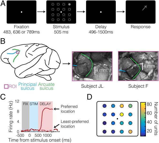
Two adult male monkeys (Macaca fascicularis) (subjects “JL” and “F”) performed an oculomotor delayed-response task (Fig. 1A) while we recorded from neuronal ensembles in the left LPFC area 8A, anterior to the arcuate sulcus and posterior to the principal, using chronically implanted 96-channel microelectrode arrays (Fig. 1B). The neural correlates of WM for spatial locations have been extensively documented in this brain region (10). The target stimulus could appear at any one of 16 possible locations, arranged in a uniformly spaced 4 × 4 grid around a central fixation point. We collected spike data from a total of 545 single units and multiunits across 12 recording sessions, out of which 417 (76%) exhibited sustained activity and selectivity during the delay epoch (P < 0.05, Kruskal–Wallis; firing rate × location) (Materials and Methods). We included both multiunits and single units in our analyses, as in similar previous studies (21, 25, 27, 34). A unit’s preferred location during a given epoch was defined as the location that elicited the largest response averaged over that epoch (Fig. 1 C and D). Subjects made incorrect choices about the stimulus location in <1% of completed trials. Only correct, completed trials were included for analysis.

Fig. 1.

Task, method, and single-cell data. (A) Overview of oculomotor delayed-response task. The arrow represents the correct saccade direction. The dashed circles indicate potential cue locations and are shown for illustrative purposes only and are not present in the task. (B) Array implantation sites and anatomical landmarks in both subjects. (C) Example delay-selective neuron. (D) Distribution of delay-selective units’ preferred locations. FIX, fixation; ROI, region of interest; STIM, stimulus.

Task-Related Modulation of Spike Count Correlations.

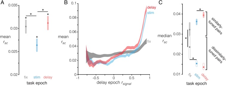
We computed spike count correlations (r_sc) between pairs of neurons (pairwise r_sc) (Materials and Methods) during the fixation, stimulus, and delay epochs. r_sc can covary with firing rate (21, 35) so, to ensure that differences in r_sc across epochs were not confounded by differences in firing rates, we implemented a distribution-matching procedure (Materials and Methods). We replicated two findings from previous studies: Mean pairwise r_sc was significantly above zero in each task epoch (Fig. 2A) (P < 0.005 for all epochs, bootstrap test) (Materials and Methods); and r_sc varied as a function of tuning similarity, which we quantified as signal correlation between pairs of neurons during the delay epoch (r_signal) (Materials and Methods) (Fig. 2B) (18, 29–33). Specifically, we found that the median pairwise r_sc was consistently larger for similarly tuned neuron pairs (defined as r_signal > 0.25) compared with dissimilarly tuned pairs (defined as r_signal < −0.25) (P < 0.001 for all epochs, bootstrap test) (Materials and Methods). We also found that mean pairwise r_sc was greater during the fixation and delay epochs compared with the stimulus epoch (Fig. 2A) (P < 0.001 for both fixation vs. stimulus and delay vs. stimulus, bootstrap test). Most importantly, we found that the relationship between r_sc and r_signal changed across task epochs (Fig. 2B); specifically, median pairwise r_sc for similarly tuned neurons was larger during the delay epoch than during the fixation and stimulus epochs (P < 0.001 for both comparisons, bootstrap test) (Fig. 2C), and median pairwise r_sc between dissimilarly tuned neurons was lower during the stimulus and delay epochs than during the fixation epoch (P < 0.001 for both comparisons, bootstrap test) (Fig. 2C). These results indicate that WM maintenance modifies pairwise r_sc in the LPFC in a manner consistent with a recurrent excitation, lateral inhibition scheme (12–17, 36).

Fig. 2.

Measures of correlated variability and its effects on WM information in full ensembles. (A) Mean pairwise r_sc (y axis) across task epochs (x axis), controlling for firing rate (SI Materials and Methods). The mean is computed across all 2,000 subsampled distributions, and shaded regions are SEM calculated using the sample size of a single subsampled distribution (n = 10,535 pairs). *P < 0.001, bootstrap test. (B) Mean r_sc for each task epoch (y axis) as a function of delay epoch r_signal (x axis). The same subsampling procedure as in A was applied, and then the r_sc of each neuron pair was binned based on its corresponding r_signal, and the mean r_sc computed in each bin. r_signal bins are size = 0.2, stepped by increments of 0.05. The shaded regions are SEM, calculated using the sample size of the corresponding r_signal bin. (C) Median r_sc for similarly tuned neuron pairs (r_signal > 0.25) and dissimilarly tuned neuron pairs (r_signal < −0.25) in each task epoch. The colored region around each point represents the bootstrapped 99.9% confidence interval of the median, derived from 2,000 bootstrap iterations. Nonoverlapping colored regions indicate P < 0.001, bootstrap test; however, pairwise comparisons that are visually ambiguous have explicitly marked (*) significant differences. FIX, fixation; STIM, stimulus.

Quantifying Information Content in Neuronal Ensembles Using Linear Decoders.

Pairwise measurements of r_sc are insufficient for predicting the effects of r_sc structure on ensemble information in large, multidimensional ensembles with heterogeneous tuning (20). Furthermore, analytical methods for determining the effects of r_sc structure on information content can be complicated to calculate for large stimulus sets and can also be inaccurate unless applied to data consisting of hundreds of trials per stimulus (20, 37). Linear decoders are demonstrably well-suited for extracting low-dimensional representations from high-dimensional neuronal ensemble data and for directly assessing the impact of r_sc structure on ensemble information content and thus offer a pragmatic solution to the issues of dimensionality and correlated variability (20, 38).

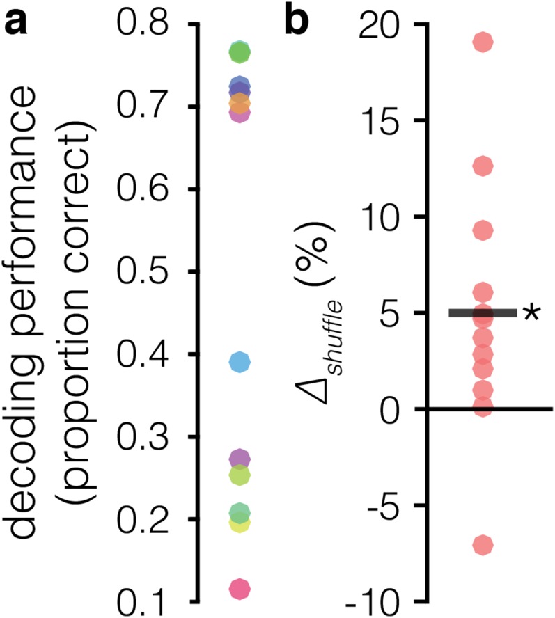
Previous studies have decoded the identity of stimuli maintained in spatial (39, 40) and nonspatial WM (8, 39) in pseudopopulations of LPFC neurons, typically using sets of 2 to 8 unique stimuli. We were able to reliably decode which of 16 target locations was being held in WM during the delay epoch by applying a linear support vector machine (SVM) (Materials and Methods) to simultaneously recorded ensemble data (Fig. S1A) (max = 77%; mean across sessions = 52%).

Fig. S1.

Decoding in full ensembles. (A) Decoding performance for full ensembles in each session. (B) Effects of removing the r_sc structure (Δ_shuffle) during the delay epoch for each session. Removing the r_sc shuffling has a net effect of improving decoding accuracy in the full ensembles (i.e., ensembles including all simultaneously recorded neurons). The black line denotes the across-session mean. *P = 0.0032, paired t test. Δ_shuffle = [(accuracy_rsc-shuffled/accuracy_rsc-intact) − 1] × 100.

Examining ensembles consisting of every simultaneously recorded neuron and/or only tuned neurons is a standard practice in neurophysiology. However, this practice assumes that all of the examined neurons contribute to coding, an assumption difficult to verify. It is possible that a subset of the recorded neurons can represent nearly as much information as the entire ensemble and that such a subset could form a “unit” of information coding that is read out by a downstream mechanism. Furthermore, the information-modifying effects of the r_sc structure have been proposed to increase with ensemble size, but most of our knowledge about these scaling effects is drawn from extrapolations of pairwise recordings, which do not necessarily predict ensemble-level effects (19–22, 41, 42). Thus, examining how information coding varies across different subsets or subensembles of simultaneously recorded neurons—what we refer to as the ensemble configuration space—could reveal insights overlooked by the constraint of analyzing only a single, fixed ensemble of all tuned neurons recorded during an experiment.

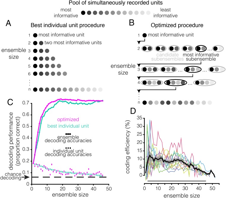
To determine how WM coding scales across ensemble configurations, we devised “ensemble construction” procedures. The procedures consisted of iteratively constructing neuronal ensembles by drawing units from the pool of all simultaneously recorded neurons and quantifying the WM information using the decoder (Fig. 3). We implemented two procedure variants. We refer to the first variant as the “best individual unit” method. This method examines the assumption that a neuronal ensemble is simply a collection of the best individually tuned neurons; accordingly, the method is agnostic to between-neuron information, such as the ensemble r_sc and r_signal structures. It was implemented as follows (Fig. 3A): We began by using the decoder to assess the WM information content of each individual unit in a single recording session. We then rank-ordered the units based on their information content. An ensemble of two neurons was constructed using the two most informative neurons, and the decoding analysis was performed on the ensemble of two neurons. This process was repeated iteratively, performing the decoding analysis using the n most informative neurons in the session, until the ensemble consisted of all of the neurons recorded in the session. The results from applying the best individual unit method to an example session are depicted in Fig. 3C (teal).

Fig. 3.

Accounting for between-neuron phenomena increases ensemble efficiency. Visualization of the (A) best individual unit ensemble construction procedure and (B) optimized ensemble construction procedure. Each circle represents a unit, and the shading represents that unit’s information content, as assessed using the decoder. (C) Decoding results for the best individual unit (teal) and optimized procedures (violet), applied to a single example session. The continuous line plot with circular markers shows the ensemble decoding accuracy (y axis) as a function of size (x axis). The square markers at the bottom of the plot denote the decoding accuracy (y axis) of the individual unit added to the ensemble at a given size (x axis). Both methods yield identical results for ensembles of the maximum size because these ensembles are identical; they consist of every simultaneously recorded unit in the session (i.e., the full ensemble). (D) Coding efficiency of the optimized method relative to the best individual unit method (y axis) as a function of ensemble size (x axis). Coding efficiency is quantified as [(accuracy_optimized/accuracy_{best individual unit}) − 1] × 100. Colored lines are values for individual sessions. The thick black line is the across-session mean, and the gray shaded area is the SEM. The gray line running along the bottom indicates ensemble sizes for which the optimized method is significantly more efficient than the best individual unit method (P < 0.05, paired t test, Hochberg-corrected).

The second variant of our ensemble construction procedure, which we refer to as the “optimized” method (Fig. 3B) (also referred to as “greedy forward selection” in the machine learning literature) (43), was designed to optimize WM information for a given ensemble size, accounting for the r_sc and r_signal structures that were ignored in the best individual unit method. The optimized method also began by rank-ordering the information content of individual neurons within a given recording session using the decoder. However, instead of starting with the two most informative individual neurons, as in the best individual unit method, we instead constructed all possible neuron pairs that contained the most informative unit. We then identified the most informative of these pairs, as assessed using the decoder. The most informative pair was then combined with each remaining neuron to generate a set of trios, from which the most informative trio was identified and used as the basis for of the most informative quartet, and so on, until the ensemble consisted of all of the neurons recorded in the session. Fig. 3C shows the results of applying the optimized method to an example session. Unlike the best individual unit method, the optimized method does not consider the information content of an individual unit in isolation but instead considers how the neuron contributes to the information content of the ensemble to which it belongs.

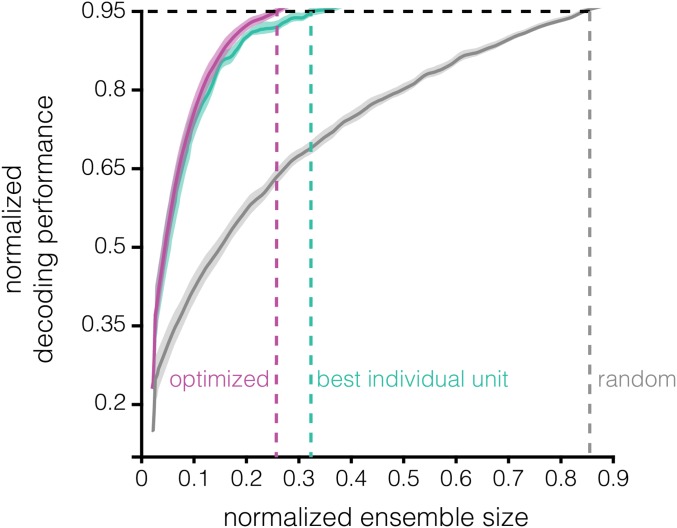
The results of the two ensemble-building methods are directly compared in Fig. 3 C and D. Notice that the optimized method yields more informative ensembles of a given size than the best individual unit method. We refer to this property—differing WM information content in ensembles of identical size—as “coding efficiency”; the optimized ensembles are more efficient than the best individual unit ensembles. Note that coding efficiency can also refer to the converse idea—identical WM information in ensembles of different size. We quantified coding efficiency as the percent change in decoding accuracy of the optimized method relative to the best individual unit method (similar to Δ_shuffle) (Materials and Methods) (Fig. 3D). The optimized method becomes significantly more efficient than the best individual unit method starting at ensemble size n = 3 (P < 0.05, paired t test, Hochberg-corrected). For certain sessions and ensemble sizes, the relative efficiency can exceed 30%. Furthermore, the decoding performance approaches saturation more quickly in the optimized ensembles (Fig. S2). Achieving 95% of maximum decoding accuracy using the optimized method requires only ∼25% of the units recorded in a given session (∼11 units) whereas the best individual unit method requires ∼33% of the units (∼14 units). In “random” ensembles—ensembles generated by randomly subsampling n units from a given recording session—∼85% of the units are necessary to reach 95% of maximum decoding accuracy. These results demonstrate that neuronal ensembles in the LPFC encode more information than single neurons, that the most informative ensembles are not necessarily composed of the most informative individual units, and that a relatively small subset of neurons can represent nearly as much WM information as the full recorded population.

Fig. S2.

Decoding saturation curves for the best individual unit vs. best subensemble methods. Normalized decoding accuracy (y axis) as a function of normalized ensemble size (x axis) is plotted for the best individual unit (teal), optimized (violet), and random (gray) ensembles. The normalized ensemble size at which normalized decoding accuracy of 0.95 is achieved is shown for the three procedures.

Effects of r_sc and r_signal Structures on WM Coding Efficiency.

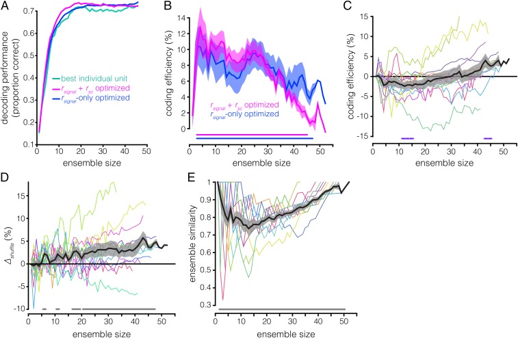
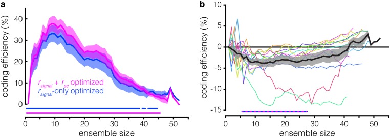
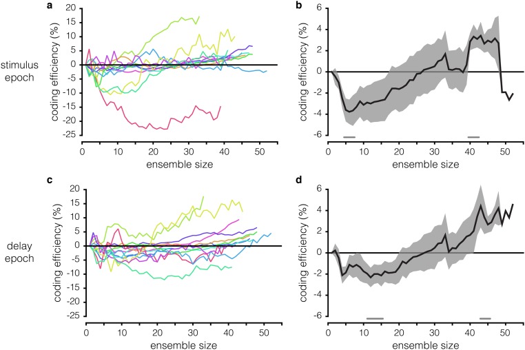
To dissociate the effects of the r_sc and r_signal structures on WM coding efficiency in the optimized ensembles, we constructed new ensembles using the optimized procedure on firing rate data from which the r_sc structure had been removed via shuffling; the classifier was trained and tested on shuffled data for each ensemble size. We then compared the information content of these “r_signal-only” ensembles with the information content of ensembles generated using the original, r_sc structure-intact data, which we now refer to as the “r_signal + r_sc” ensembles. The results for all three methods (best individual unit, r_signal + r_sc-optimized, and r_signal-only–optimized) applied to an example session are compared in Fig. 4A. The r_signal-only ensembles contain significantly more WM information than the best individual unit ensembles across sizes ranging from 2 to 47 neurons (P < 0.05, paired t test, Hochberg-corrected) (Fig. 4B). However, the effect of the r_sc structure is variable: The r_signal + r_sc ensembles are more efficient than the r_signal-only ensembles at smaller ensemble sizes whereas this effect inverts at larger ensemble sizes (P < 0.05 for ensemble sizes of 11 to 15 and 43 to 45 neurons, paired t test, Hochberg-corrected) (Fig. 4 B and C). These changes in WM coding efficiency effected by the r_sc structure can reach ±15% across different recording sessions and ensemble sizes (Fig. 4C), enough to double (or nullify) efficiency increases afforded by the r_signal structure alone. These results indicate that the r_sc structure significantly impacts WM coding and can do so in a manner that varies nonmonotonically with ensemble size. These results cannot be ascribed to idiosyncrasies of the SVM decoder because repeating the same analyses using logistic regression yields similar results (Fig. S3). We also found a similar—though less consistent—effect during stimulus presentation, with considerably greater session-to-session variability (Fig. S4).

Fig. 4.

Effects of r_sc structure on ensemble coding efficiency and composition. (A) Decoding accuracy (y axis) as a function of ensemble size (x axis) for the best individual unit (teal), r_signal + r_sc (violet), and r_signal-only (blue) methods for the same example session as in Fig. 3C. Note that, for the r_signal-only ensembles, the classifier was trained and tested on r_sc-shuffled data whereas, for the r_signal + r_sc and best individual unit ensembles, the classifier was trained and tested on r_sc-intact data. (B) Coding efficiency of r_signal + r_sc ensembles and r_signal-only ensembles, relative to the best individual unit ensembles (y axis), as a function of ensemble size (x axis). The violet line running along the bottom indicates ensemble sizes for which the r_signal + r_sc ensembles are significantly more efficient than the best individual unit ensembles (P < 0.05, paired t test, Hochberg-corrected); the blue line is similar, but for r_signal-only ensembles vs. best individual unit ensembles. Note that the coding efficiency of r_signal + r_sc ensembles relative to best individual unit ensembles was previously shown in Fig. 3D. (C) Coding efficiency of r_signal-only ensembles relative to r_signal + r_sc ensembles; similar to Fig. 3D. A positive value indicates that shuffling out the r_sc structure improves decoding. The striped blue and violet lines running along the bottom indicate ensemble sizes for which the efficiency of r_signal + r_sc ensembles and r_signal-only ensembles are significantly different (P < 0.05, paired t test, Hochberg-corrected). (D) Decoding performance of r_sc-shuffled vs. r_sc-intact ensembles (∆_shuffle, y axis) as a function of ensembles size (x axis) for random ensembles. Ensembles were generated by randomly subsampling n units from the full recorded population in a given session. The gray lines running along the bottom indicate ensemble sizes for which the r_sc-shuffled vs. r_sc-intact ensembles are significantly different (P < 0.05, paired t test, Hochberg-corrected). (E) Similarity between r_signal + r_sc ensembles and r_signal-only ensembles (y axis) as a function of ensemble size (x axis). Ensemble similarity is quantified as the proportion of units common to the two ensembles for a given size. Note that ensemble similarity is 1 for ensembles of size n = 1, and for the largest ensemble size in a given session, because both ensemble-building procedures begin with the same unit, and the largest ensemble in each session consists of every simultaneously recorded unit in that session. The gray line running along the bottom indicates ensemble sizes for which the similarity of the r_signal + r_sc ensembles and r_signal-only ensembles is significantly less than 1 (P < 0.05, z-test of proportion, Hochberg-corrected).

Fig. S3.

Effects of r_sc structure on ensemble coding efficiency when using logistic regression. (A) Similar to Fig. 4B, but using logistic regression instead of SVM. Coding efficiency of r_signal + r_sc ensembles and r_signal-only ensembles, relative to the best individual unit ensembles (y axis), as a function of ensemble size (x axis). The violet line running along the bottom indicates ensemble sizes for which the r_signal + r_sc ensembles are significantly more efficient than the best individual unit ensembles (P < 0.05, paired t test, Hochberg-corrected); the blue line is similar, but for r_signal-only ensembles vs. best individual unit ensembles. (B) Coding efficiency of r_signal-only ensembles relative to r_signal + r_sc ensembles; similar to Fig. 4C, but using logistic regression instead of SVM. A positive value indicates that shuffling out the r_sc structure improves decoding. The striped blue and violet line running along the bottom indicates ensemble sizes for which the efficiency of r_signal + r_sc ensembles and r_signal-only ensembles is significantly different (P < 0.05, paired t test, Hochberg-corrected).

Fig. S4.

Effects of the r_sc structure during the stimulus vs. delay epochs. (A) Similar to Fig. 4C, but during the stimulus epoch. Coding efficiency of r_signal-only ensembles relative to r_signal + r_sc ensembles for individual sessions. A positive value indicates that shuffling out the r_sc structure improves decoding. Each colored line is an individual session. (B) Across-session mean coding efficiency of r_signal-only ensembles relative to r_signal + r_sc ensembles during the stimulus epoch. The gray lines running along the bottom indicate ensemble sizes for which the efficiency of r_signal + r_sc ensembles and r_signal-only ensembles is significantly different (P < 0.05, paired t test, Hochberg-corrected). (C) Identical data as Fig. 4C, presented again here for comparison with stimulus epoch data. Coding efficiency of r_signal-only ensembles relative to r_signal + r_sc ensembles for individual sessions. (D) Identical data as Fig. 4C, presented again here for comparison with stimulus epoch data. Across-session mean coding efficiency of r_signal-only ensembles relative to r_signal + r_sc ensembles.

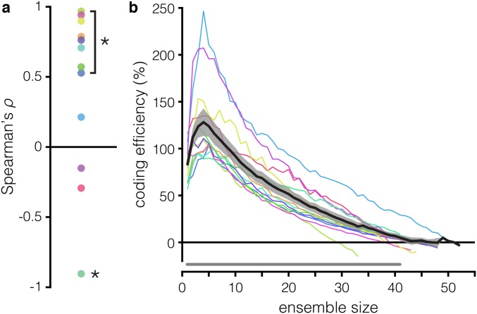
It is possible that the observed effects of the r_sc structure on WM coding are simply a property of an ensemble’s size, regardless of whether the ensemble is optimized for WM representation. To resolve this ambiguity, we compared the decoding performance of the random ensembles in which r_sc structure was intact vs. shuffled (Fig. 4D). We found that shuffling out the r_sc structure significantly improved decoding in most ensembles of six or more units (P < 0.05, paired t test, Hochberg-corrected) and that the magnitude of the decoding improvement was robustly and significantly correlated with the size of the ensemble in 8 out of 12 recording sessions (Spearman’s ρ ≥ 0.53; P < 0.001) (Fig. S5A). Although the r_sc structure seems to consistently impair decoding at the largest ensemble sizes (Fig. S5B), these results demonstrate that WM coding in a neuronal ensemble consisting of randomly selected neurons will be impaired by the r_sc structure in a manner proportional to the size of the ensemble but that the r_sc structure can actually improve WM coding in r_sc + r_signal-optimized ensembles.

Fig. S5.

Δ_shuffle and coding efficiency in random vs. optimized ensembles. (A) Δ_shuffle and ensemble size are correlated in random ensembles. The Spearman rank correlation coefficient (ρ) between ensemble size and Δ_shuffle in random ensembles, for each of the 12 recording sessions. A positive correlation indicates that shuffling out the r_sc structure increases decoding accuracy more in larger ensembles. *P < 0.01, Spearman correlation. (B) r_signal + r_sc ensembles are more efficient than random ensembles at nearly all ensemble sizes. Coding efficiency of the r_signal + r_sc ensembles relative to random ensembles (y axis) as a function of ensemble size (x axis). A positive value indicates that the r_signal + r_sc ensembles are more efficient for a given ensemble size. The gray line running along the bottom indicates ensemble sizes for which the r_signal + r_sc ensembles are significantly more efficient than the random ensembles (P < 0.05, paired t test, Hochberg-corrected).

Different Ensemble Configurations Optimize WM Coding When the r_sc Structure Is Intact vs. Removed.

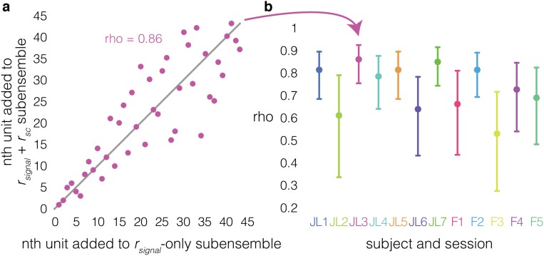
The previous results demonstrate that accounting for an ensemble’s r_sc structure can significantly alter estimates of its WM information content. A complementary question is whether accounting for the r_sc structure also alters estimates of individual neurons’ contributions to an ensemble’s WM coding. Are ensembles that maximize coding efficiency when the r_sc structure is intact composed of the same neurons that maximize coding efficiency when the r_sc structure is shuffled out? To answer this question, we examined the proportion of units common to both the r_signal + r_sc and r_signal-only ensembles for each ensemble size (Fig. 4E). The proportion is significantly less than 1 for ensemble sizes of 2 to 50 neurons (P < 0.05, z-test of proportions, Hochberg-corrected), indicating that the ensembles generated by the two methods are not identical; the similarity within an individual session can be as low as 33%. The r_signal + r_sc and r_signal-only procedures also recruited units into ensembles in different sequences (Spearman’s ρ < 1 in all sessions, mean ρ = 0.713; P < 0.05, Bonferroni-corrected) (Fig. S6). These results demonstrate that different subpopulations of neurons optimize WM coding when the intrinsic r_sc structure is present vs. when it is absent although some neurons strongly contribute to WM coding regardless of an ensemble’s r_sc structure.

Fig. S6.

Ensemble construction sequence correlation shows that different ensembles maximize WM information when the r_sc structure is intact vs. removed. (A) Sequence order correlation between r_signal + r_sc ensembles (y axis) and r_signal-only ensembles (x axis) for an example session. The nth unit added to the ensemble in the r_signal-only method (x axis) is plotted against the n at which it was added to the ensemble in the r_signal + r_sc method. For example, the fifth unit added in the r_signal-only method is added fourth in the r_signal + r_sc method. If the sequence in which the two methods added units was identical, all of the points would fall along the unity line (gray), and the Spearman rank correlation coefficient (ρ) between the two sequences would equal 1, indicating that identical ensembles maximize WM information regardless of whether the r_sc structure is intact. Likewise, ρ = 0 means that the relationship between the sequences is random; the ensembles that maximize WM information when the r_sc structure is intact are entirely distinct from the ensembles that maximize WM information when the r_sc structure has been removed. (B) Spearman rank correlation coefficient (ρ) between the r_signal + r_sc ensembles and r_signal-only ensembles (y axis) for each session (x axis). Error bars are Bonferroni-corrected 95% confidence intervals. The correlation between ensemble sequences is significantly less than 1 in every session (P < 0.05, Bonferroni-corrected), indicating that the ensembles that maximize WM information when the r_sc structure is intact are built in a different sequence than the ensembles that maximize WM information when the r_sc structure has been removed. The range of ρ values (0.53 to 0.86) shows that there is some degree of similarity to the sequences in which the two methods recruit neurons to the ensembles.

Ensembles Optimized for WM Representation Are r_signal-Diverse and Anatomically Dispersed.

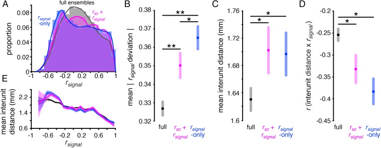
One of our earlier analyses demonstrated that near-maximum decoding performance can be achieved with a relatively small proportion of recorded units and that accounting for an ensemble’s r_signal and/or r_sc structure can further enhance WM coding. If the WM coding is optimized in these ensembles by maximizing their representation of the stimulus space, their r_signal distributions should be broader than those of the full recorded ensembles. We tested this hypothesis by examining the r_signal + r_sc and r_signal-only ensembles that achieved ≥95% of maximum decoding performance in each session (which we refer to as “near-max” ensembles). Indeed, we found that the r_signal distributions of the near-max r_signal + r_sc ensembles, r_signal-only ensembles, and full ensembles were all significantly different from each other (Fig. 5A) (P << 0.001 for all comparisons, χ² test, Bonferroni-corrected). The width of the r_signal distribution, measured as the mean absolute deviation (Materials and Methods), was larger for the near-max r_signal + r_sc and r_signal-only ensembles than for all units (Fig. 5B) (P << 0.001 for both, F test, Bonferroni-corrected) and larger in the r_signal-only than the r_signal + r_sc ensembles (P = 0.01, F test).

Fig. 5.

Ensembles optimized for WM representation are r_signal-diverse and anatomically dispersed. (A) r_signal distributions for the full ensembles (gray; n = 12,222 units), near-max r_signal + r_sc ensembles (violet; n = 2,414), and near-max r_signal-only ensembles (blue; n = 2,724), pooled across all sessions. All three distributions are significantly different from each other (P << 0.001, χ² test, Bonferroni-corrected; computed using nonoverlapping bins of size = 0.1). (B) Mean |r_signal deviation| in the full (gray), near-max r_signal + r_sc (violet), and near-max r_signal-only ensembles (blue). r_signal deviation is defined as the difference between a unit pair’s r_signal and the mean r_signal of the ensemble to which the unit pair belongs. **P << 0.001, Bonferroni-corrected, *P = 0.01, F test (SI Materials and Methods). Shaded regions represent Bonferroni-corrected 95% comparison intervals between group means (SI Materials and Methods). (C) Mean interunit distance in each of the three ensemble groups. *P < 0.005, F test, Bonferroni-corrected. Shaded regions represent Bonferroni-corrected 95% comparison intervals between group means. (D) Correlation between interunit distance and r_signal in the three ensemble groups. *P < 0.005, bootstrap test. Shaded regions represent bootstrapped 95% confidence intervals. (E) Mean interunit distance (y axis) as a function of r_signal in each of the ensemble groups, computed using nonoverlapping r_signal bins of size 0.1. Shaded region denotes SEM.

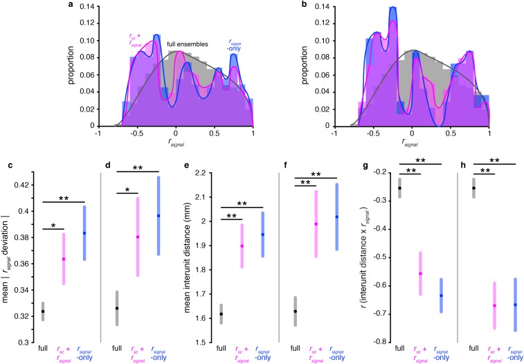
Prior studies have reported weak topography for visual (44, 45) and mnemonic (29) space in LPFC; units’ tuning similarity and the anatomical distance between them—the “interunit distance”—are negatively correlated. If the optimized ensembles reflect this topography, their broader representation of the stimulus space means that they should encompass larger regions of cortex relative to the full recorded ensembles. Indeed, we found that the mean distance between units—or interunit distance—was larger in the near-max r_signal + r_sc and r_signal-only ensembles than the full ensembles (Fig. 5C) (P < 0.005 for both, F test, Bonferroni-corrected) (Materials and Methods). We also found that topography in the optimized ensembles was enhanced compared with the full ensembles (Fig. 5D); the correlation between interunit distance and r_signal was significantly stronger in the near-max r_signal + r_sc ensembles (r = −0.33) and r_signal-only ensembles (r = −0.38) compared with the full ensembles (r = −0.26; P < 0.005 for both, bootstrap test). A potential explanation for this difference is that the distance between units with negative r_signal is larger in the optimized ensembles (Fig. 5E). Remarkably, the mean interunit distance can reach 2.5 mm in the near-max ensembles. Considering that cortical columns in the LPFC could span ∼0.7 mm (46), this result suggests that optimal ensembles extend across several cortical columns. These results link the spatial mnemonic topography of LPFC to principles of WM coding. They also demonstrate the utility of accounting for neuronal information content when examining cortical organization, compared with approaches that focus on neuronal tuning characteristics while leaving their effects on information implicit. These findings are also robust to the choice of near-max value because repeating the analyses with different thresholds yielded similar results (Fig. S7).

Fig. S7.

Functional anatomy analyses are consistent even when using different decoding saturation thresholds. (A) r_signal distributions for the full ensembles (gray), near-max r_signal + r_sc ensembles (violet), and near-max r_signal-only ensembles (blue), pooled across all sessions. Identical to Fig. 5A, but using a threshold of 90% of maximum decoding. The r_signal + r_sc ensemble and r_signal-only ensemble distributions are both significantly different from the full ensemble distributions (P < 0.001, χ² test, Bonferroni-corrected; computed using nonoverlapping bins of size = 0.1). (B) Identical to A, but using a threshold of 80% of maximum decoding. All three distributions are significantly different from each other (P < 0.001, χ² test, Bonferroni-corrected; computed using nonoverlapping bins of size = 0.1). (C) Mean |r_signal deviation| in the three categories of ensembles. Identical to Fig. 5B, but using a threshold of 90% of maximum decoding. r_signal deviation is defined as the difference between a unit pair’s r_signal and the mean r_signal of the ensemble to which the unit pair belongs. Shaded regions represent Bonferroni-corrected 95% comparison intervals between group means (Materials and Methods). (D) Identical to C, but using a threshold of 80% of maximum decoding. (E) Mean interunit distance in each of the three ensemble groups. Identical to Fig. 5C, but using a threshold of 90% of maximum decoding. Shaded regions represent Bonferroni-corrected 95% comparison intervals between group means. (F) Identical to E, but using a threshold of 80% of maximum decoding. (G) Correlation between interunit distance and r_signal in the three ensemble groups. Identical to Fig. 5D, but using a threshold of 90% of maximum decoding. Shaded regions represent bootstrapped 95% confidence intervals. (H) Identical to G, but using a threshold of 80% of maximum decoding. *P = 0.01, **P << 0.001, F test (Materials and Methods).

Nonselective Units Can Improve WM Coding by Modifying the r_sc Structure.

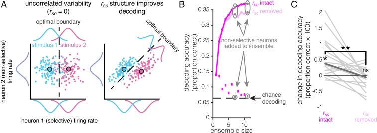
Given our observation that the r_sc structure can significantly affect the information content of a neuronal ensemble during WM, it is possible that neurons that do not contain task-related information in isolation could still influence the information content of an ensemble by modifying the r_sc structure (Fig. 6A). The r_signal distribution of the r_signal + r_sc ensembles in Fig. 6A contains a peak near r_signal = 0, unlike the r_signal-only ensembles, suggesting that units with orthogonal and/or weak selectivity may contribute more to WM coding when the r_sc structure is intact. Indeed, nonselective units were sometimes added to ensembles before selective units, and before decoding performance saturated (Fig. 6B). To test whether these units were increasing ensemble WM information by modifying the r_sc structure, we identified all of the non delay-selective units (P ≥ 0.05, one-way Kruskal–Wallis ANOVA with stimulus location as the factor) that were added before decoding performance saturation in the r_signal + r_sc ensembles (Fig. 6B) (16 units in total). We then compared the amount of information these units contributed to an ensemble before and after shuffling out the r_sc structure (Fig. 6C) (Materials and Methods). Removing the r_sc structure significantly decreased the amount of WM information contributed by these units (P < 0.01, signed rank test, paired), and the amount of WM information contributed after shuffling was not significantly different from zero (P = 0.43, Wilcoxon signed rank test, unpaired; additional descriptive statistics and control analyses for these units are provided in Fig. S8). We also found 15 nonselective, noise-shaping neurons during the stimulus epoch. Only one of the nonselective, noise-shaping neurons was common to both epochs. However, the decoding improvement contributed by these neurons, both before and after removing the r_sc structure, was more consistent during the delay than the stimulus epoch (Fig. S9). These results demonstrate the existence of nonselective noise-shaping neurons: neurons that do not contain task-related information in isolation but increase the information content of an ensemble entirely through modifying the r_sc structure.

Fig. 6.

Nonselective neurons can increase ensemble information by modifying the r_sc structure. (A) Two-neuron conceptual diagram of how a nonselective neuron could increase ensemble information content. In the first scenario (Left), one neuron differentiates between two stimuli (i.e., is selective; stimuli are denoted by blue and pink), and the other neuron does not (i.e., is not selective). The response variability of the two neurons is not correlated (i.e., r_sc = 0). In the second scenario (Right), the individual neurons’ properties are identical, yet correlated response variability (i.e., the r_sc structure) improves discrimination between the two stimuli relative to the uncorrelated scenario. (B) The continuous line plots with circular markers show the ensemble decoding accuracy (y axis) as a function of size (x axis) for the r_sc + r_signal-optimized method for a single example ensemble, before decoding saturation, for r_sc-intact data (magenta) and r_sc-shuffled data (pale magenta). The square markers at the bottom of the plot denote the decoding accuracy (y axis) of the individual unit added to the ensemble at a given size (x axis). Notice units that are added to the population that are not selective (gray). (C) Change in decoding accuracy from adding nonselective units to presaturation ensembles (y axis) when the r_sc structure is intact (left) and removed (right). Each line is the change for an individual unit. The bolded line is the median. Removing the r_sc structure eliminates the information gain contributed by these units. *P = 0.001, signed-rank test; **P < 0.003, paired signed-rank test; ns (not significant), P = 0.43, signed-rank test; n = 16.

Fig. S8.

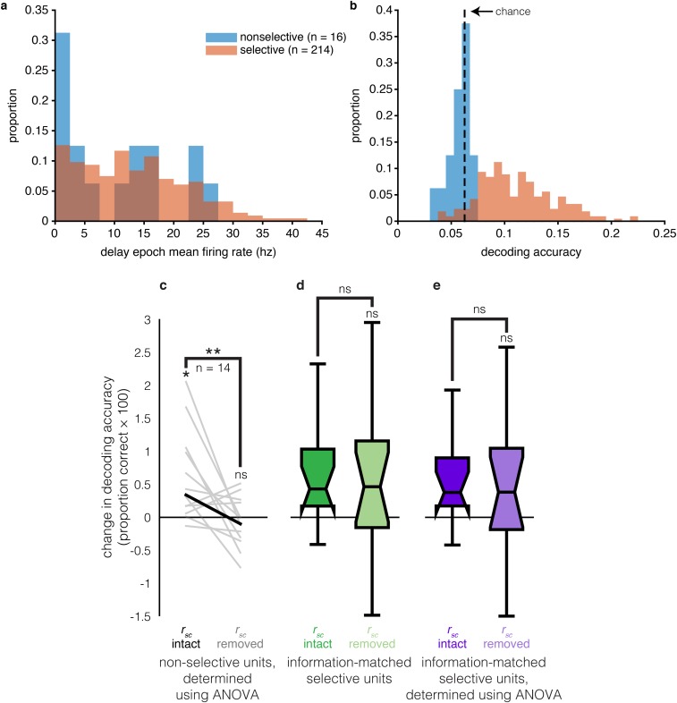
Descriptive statistics and control analyses for nonselective noise-shaping units. (A) Histogram of delay epoch firing rates of nonselective (P ≥ 0.05, Kruskal–Wallis ANOVA; blue) and selective (P < 0.05, Kruskal–Wallis ANOVA; orange) units in best ensembles. Firing rate bins are plotted on the x axis, and bin counts are plotted on the y axis. (B) Histogram of delay epoch decoding accuracies of nonselective and selective units in best ensembles. Decoding accuracy bins are plotted on the x axis, and bin counts are plotted on the y axis. (C) Parametric selectivity control. We reran the analysis in Fig. 6, defining selectivity as P < 0.05, ANOVA, instead of Kruskal–Wallis ANOVA. The change in decoding accuracy from adding nonselective units to best ensembles (y axis) is compared when the r_sc structure is intact (left) and removed (right). Each line is the change for an individual unit. The bolded line is the median. Similar to when using a nonparametric measure of WM selectivity, removing the r_sc structure eliminates the information gain contributed by these units. *P = 0.001, signed-rank test; **P = 0.01, paired signed-rank test; ns, P = 0.58, signed-rank test; n = 13. (D) Selective unit control. We used a distribution-matching procedure (Materials and Methods) to obtain a distribution of WM-selective units (P < 0.05, Kruskal–Wallis ANOVA) that contribute equivalent amounts of information to an ensemble as the nonselective units and performed a similar analysis as in Fig. 6. The center of each box is the median, and the notches extend from the median ± 1.57(q₃ − q₁)/√n, where q₃ is the 75th percentile, q₁ is the 25th percentile, and n = 13, the sample size of a single matched distribution. The bottom box edge = q₁, top edge = q₃, and the whiskers extend ∼99.3% distribution coverage. Removing the r_sc structure does not change the magnitude of information added to the ensemble by these units (P > 0.05, bootstrap test) (Materials and Methods); thus, it is not simply the case that units that weakly improve ensemble information do so by modifying the r_sc structure. ns, P > 0.05, bootstrap test. (E) Selective unit plus parametric selectivity control. Same as b, but defining selectivity as P < 0.05, ANOVA, instead of Kruskal–Wallis ANOVA. The results are similar for the two methods. ns (not significant), P > 0.05, bootstrap test.

Fig. S9.

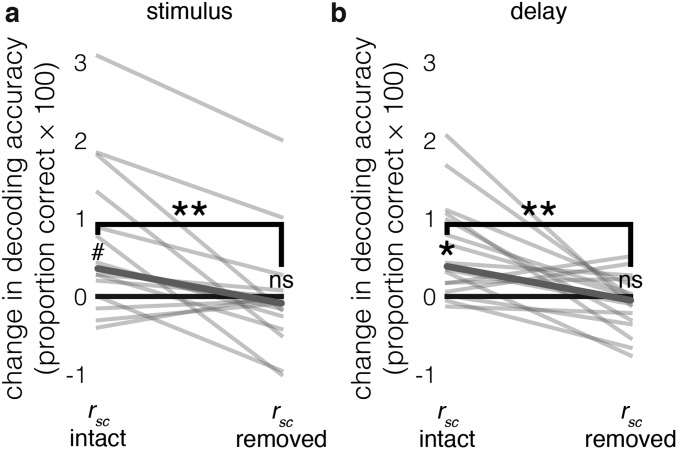
Comparison of untuned noise-shaping neurons during stimulus and delay epochs. (A) Similar to Fig. 6C, but during the stimulus epoch. Change in decoding accuracy from adding nonselective units to presaturation ensembles (y axis) when the r_sc structure is intact (left) and removed (right). Each line is the change for an individual unit. The bolded line is the median. ^#P = 0.013, signed-rank test; **P < 0.003, paired signed-rank test; ns, P > 0.05, signed-rank test; n = 15. (B) Contribution of untuned, noise-shaping units during the delay epoch. Identical to Fig. 6C, presented again here for comparison with stimulus epoch data. *P = 0.001, signed-rank test, **P < 0.003, paired signed-rank test; ns (not significant), P > 0.05, signed-rank test; n = 16.

Discussion

By using microelectrode arrays to record from ensembles of LPFC neurons, we were able to elucidate the effects of the r_sc structure on WM coding and, more generally, how WM is represented in neuronal ensembles. We found that the relationship between r_sc and r_signal during WM maintenance was as predicted by connection topography in which similarly tuned neurons are recurrently excitatory and dissimilarly tuned neurons are mutually inhibitory. Using a linear decoder, we found that removing the r_sc structure could increase or decrease the information content of the neuronal ensemble, depending on the size and composition of the ensemble. Consistent with previous findings, WM fidelity in ensembles of randomly selected neurons was impaired by the r_sc structure, and the magnitude of the impairment was proportional to the size of the ensemble. However, the intrinsic r_sc structure improved WM coding in smaller neuronal ensembles of neurons optimized for WM representation (r_signal + r_sc ensembles). The r_signal + r_sc ensembles consisted of different neurons than ensembles optimized for WM representation in the absence of the r_sc structure (r_signal-only ensembles). The r_signal + r_sc ensembles had a broader r_signal distribution, were more anatomically dispersed, and exhibited stronger topography than the full population of recorded LPFC units. Finally, we found that individual units that did not encode WM in isolation (nonselective neurons) could still contribute to WM coding when part of an ensemble by altering the ensemble’s r_sc structure.

Recurrent Network Dynamics During WM Coding.

WM representations in the LPFC are hypothesized to be maintained by a network structure of recurrent excitation and lateral inhibition (12–18). The resulting dynamics should manifest as changes in r_sc during WM maintenance (delay epoch) relative to other epochs. We observed this phenomenon in our data—mean r_sc is lower during the stimulus epoch compared with the delay epoch. A previous experiment (30) reported this trend but did not find a significant effect, perhaps due to a smaller sample size (295 pairs, compared with our 10,535 pairs). A second prediction is that WM maintenance should modify r_sc as a function of r_signal; r_sc should be lower between neurons with dissimilar tuning than neurons with similar tuning (18, 29–33). Indeed, we found that the relationship between r_sc and r_signal changed as predicted during the delay, compared with the fixation and stimulus epochs (Fig. 2B). Our findings indicate that WM maintenance modulates the r_sc structure of LPFC neuronal ensembles in a manner consistent with recurrent excitation and lateral inhibition.

Decoding WM Representations from LPFC Neuronal Ensembles.

A prior study showed that using a pseudopopulation (asynchronously recorded neurons) of the eight most informative LPFC neurons to decode spatial WM information during a match/nonmatch WM task yielded nearly identical results as using the entire 600-neuron pseudopopulation (39). We also showed that a small subensemble of the most informative neurons contain nearly as much WM information as the full recorded population. Importantly, we demonstrated that accounting for the r_sc structure increases ensemble efficiency; thus, pseudopopulation analyses likely overestimate the number of neurons required to achieve a given decoding accuracy.

A second study (40) using simultaneous recordings from 32 electrodes was also able to decode which of eight locations was being remembered during a spatial WM task. However, their study was primarily concerned with how cortical depth affected the ability to decode a remembered location from local field potentials (LFPs) and contained minimal analysis of spiking activity or the impact of neuronal ensemble composition on WM coding.

Effects of r_sc and r_signal Structures on WM Coding.

The observed patterns of r_sc and r_signal are thought to be indicative of a network structure that stabilizes WM representations over time (18, 36, 47). Our results demonstrate that these correlations can also affect the readout of WM representations from neuronal ensembles: If WM representations are read out from optimized ensembles, then the network correlation structure will favor WM coding; however, if WM representations are read out from ensembles that are “suboptimal,” then the correlation structure could impair WM coding. Our experiment shows that these changes in ensemble information content can reach 20%. Thus, a mechanism that is thought to temporally stabilize WM representations can also affect the ability to read out these representations. Note that additional discussion on how our findings extend to larger neuronal ensembles and on the effects of spike sorting in our analyses can be found in SI Discussion.

Effects of the r_sc Structure on Information in Non-WM Tasks.

Reports of the effects of ensemble r_sc structure on information content vary significantly in sign and magnitude (19, 22, 24, 27, 42, 48, 49); our results can help reconcile these disparate accounts. For example, previous studies that applied decoding techniques to simultaneously recorded ensembles found that removing the r_sc structure decreased decoding accuracy for grating orientation (48) and remembered location (49) whereas another study reported a positive effect of pairwise r_sc on information coding (32). Moreover, spatial attention increases signal-to-noise primarily by reducing r_sc (25–27). We found that the effect of r_sc structure on ensemble information varied dramatically depending on an ensemble’s size and composition; removing the r_sc structure from the full recorded ensembles increased decoding accuracy, but removing the r_sc structure from the most informative subensembles decreased decoding accuracy. The discrepancies across previous studies may arise from the location in configuration space of the neuronal ensembles under investigation (50). Importantly, they should caution us against making broad conclusions concerning how variables such as r_sc shape information transmission across brain areas. To fully clarify this issue one must identify which neurons are contributing to coding, which poses a significant technical challenge.

Our ensemble construction procedures were designed in part to sidestep the challenge of identifying which neurons contribute to coding and to allow us to characterize the system at specific states of interest. One may argue that we did not examine the full ensemble configuration space. Such an undertaking would be computationally infeasible; there are ∼10¹⁵ unique ensembles that could be created from 50 neurons. Thus, our results may actually underestimate the true range of effect sizes. Nevertheless, even a limited search of the full configuration space demonstrates the importance of the r_sc structure to WM coding in LPFC neuronal ensembles.

Noise-Shaping Units.

Neurophysiological studies typically assume that, if an ensemble codes for some behavior, the individual neurons constituting that ensemble will also code for that behavior when examined in isolation. This assumption is implicit in the method that forms the bedrock of neurophysiological research: serial recording of individual neurons. However, this approach cannot account for simultaneity between neurons. The use of large-scale simultaneous ensemble recordings allowed us to find nonselective noise-shaping neurons: neurons that are not selective for a remembered location but can improve the fidelity of WM representation in an ensemble by modifying the ensemble’s r_sc structure (Fig. 6A). A similar phenomenon was shown in a prior fMRI study; voxels that do not contain stimulus information in isolation can improve decoding when part of an “ensemble” of voxels (51). Their study and ours seem to report two different instances of the same general property of information coding in multidimensional systems: Features (e.g., voxels or neurons) that do not contain information in isolation can still modify the amount of information in a system to which they belong by changing the structure of correlated variability. It remains to be observed whether nonselective noise-shaping neurons contribute to information coding in other tasks and brain regions.

SI Discussion

Effects of Spike Sorting.

As in prior similar studies of the effects of r_sc on neuronal information coding, we included both single units and multiunits for analysis (21, 25, 27, 34), which provided the dual advantages of greater statistical power and a larger range of ensemble sizes across which to examine the effects of the r_sc structure. One caveat of this approach is that measurements of r_sc are known to be smaller for single units than for multiunit clusters, which constitute the majority of our dataset. However, our observed mean r_sc values are similar to reports in prior studies of WM in the LPFC that exclusively examined single units, in which mean r_sc ranged from ∼0.02 to 0.06, depending on the task epoch (30, 31). Our observed r_sc values were also similar to two prior studies conducted in our laboratory that used identical subjects, microelectrode arrays, and microelectrode array implantation sites as the present study (27, 45). One of these studies (27) found that the effects of r_sc on decoding spatial attentional information were robust to changes in spike sorting; the r_sc structure impaired SVM decoding of attended location whether or not the activity on an electrode was sorted into separate single unit and multiunit clusters, or remained a unitary channel of threshold crossings. Because we replicated previous findings, and observed ranges of values (e.g., r_sc, Δ_shuffle) in accordance with similar previous studies, we doubt that our results can be ascribed entirely to the inclusion of multiunit clusters in our dataset.

Generalization to Larger Ensembles.

We demonstrated that decoding performance of an ensemble can be improved by adding neurons that are not the most informative in isolation. However, this effect seems to be maximized at ensemble sizes of ∼3 to 30 neurons (e.g., Fig. 3D). The origin of this effect seems to be that it benefits decoding to maximize the width of an ensemble’s r_signal distribution (e.g., Fig. 5); if there is a stimulus that few neurons in an ensemble are selective for, it can be more beneficial to add a neuron that is weakly selective for the underrepresented stimulus than to add a neuron that is strongly selective for a stimulus that is already well-represented by the ensemble. The question remains whether this effect is simply an artifact of the sample size available for analysis and whether it would extend to larger ensemble sizes. Given that this effect arises from the selectivity statistics of the population of recorded neurons, we expect it to scale to larger ensembles so long as the statistics of the population remain similar, with the following caveats. First, this effect will depend on the size of the stimulus space (i.e., the number of unique stimuli that need to be decoded). As the size of the stimulus space increases, so does the need to represent it. In the extreme example of two stimuli to decode, this effect should not exist. Second, as ensemble decoding approaches saturation (i.e., 100%), the decoding improvement from adding neurons to the ensemble will become negligible, rendering arbitrary the choice of which neuron is “optimal” to add to the ensemble. A generalized solution for determining the ensemble size at which decoding saturates is beyond the scope of this study; however, it depends on many variables, including the size of the stimulus space, the selectivity statistics of the neurons in the ensemble, and the number of trials in the dataset.

Conclusion

We leveraged the simultaneous multineuron recording capabilities of microelectrode arrays to elucidate how WM is coded in LPFC neuronal ensembles. We found that the structure of the correlated variability (r_sc) supports current computational models of how sustained activity emerges in WM networks. A great deal of the power of modeling studies lies in their ability to explore parameter spaces, and we devised our ensemble construction procedures in an attempt to create an empirical analog of this capability. Applying these procedures revealed that the size, r_signal structure, and r_sc structure of an ensemble can profoundly impact WM coding. We also found that LPFC neuronal ensembles that optimize the coding of remembered locations are heterogeneously tuned and anatomically dispersed. Finally, we demonstrated that a ubiquitous assumption in neurophysiological studies—that only “selective” neurons contribute to information coding—is not justified in LPFC networks; nonselective neurons can contribute to information coding by shaping the r_sc structure. More generally, our results emphasize the relevance of ensemble-level phenomena in building a comprehensive understanding of brain networks.

Materials and Methods

Ethics Statement.

The animal care and ethics are identical to those in ref. 45, were in agreement with Canadian rules and regulations, and were preapproved by the McGill University Animal Care Committee. Full details can be found in SI Materials and Methods.

Task.

Trials were separated into four epochs: fixation, stimulus presentation (stimulus), delay, and response (Fig. 1A). The animal initiated a trial by maintaining gaze on a central fixation spot (0.08 degrees²) and pressing a lever; the subject needed to maintain fixation within 1.4° of the spot until cued to respond. The fixation period lasted either 483, 636, or 789 ms, determined randomly at the beginning of each trial. After fixation, a sine-wave grating (2.5 Hz/degree, 1° diameter, vertical orientation) appeared at one of 16 randomly selected locations for 505 ms. The potential stimulus locations were arranged in a 4 × 4 grid, spaced 4.7° apart, centered around the fixation point. The stimulus period was followed by a randomly variable delay period of 496 to 1,500 ms. The delay period ended and the response period commenced when the fixation point was extinguished, cuing the animal to make a saccade to the location of the previously presented stimulus and then to release the lever. The animal had 650 ms to respond. Successful completion of the trial yielded a juice reward. The minimum duration between trials was 300 ms. Fixation breaks during the trial or failure to saccade to the target in the allotted time resulted in immediate trial abortion without reward and a delay of 3.5 s before the next trial could be initiated.

Experimental Setup.

The experimental setup is identical to those in refs. 27 and 45. Full details can be found in SI Materials and Methods.

Microelectrode Array Implant.

As in refs. 27 and 45, we chronically implanted a 10 × 10, 1.5-mm microelectrode array (Blackrock Microsystems LLC) (52, 53) in each monkey’s left LPFC—anterior to the knee of the arcuate sulcus and caudal to the posterior end of the principal sulcus (area 8a) (Fig. 1B). Detailed surgical procedures can be found in ref. 45.

Recordings and Spike Detection.

Data were recorded using a Cerebus Neuronal Signal Processor (Blackrock Microsystems LLC) via a Cereport adapter. Spike waveforms were detected online by thresholding. The extracted spikes (48 samples at 30 kHz) were resorted manually in OfflineSorter (Plexon Inc.). The electrodes on each MEA were separated by at least 0.4 mm and were organized into three blocks of 32 electrodes. We collected data from one block during each recording session. Detailed recording procedures can be found in ref. 45. We collected spike data across 12 recording sessions (7 in JL, 5 in F), yielding a total of 545 units: 164 single neurons (99 in JL, 65 in F) and 381 multiunits (221 in JL, 160 in F). Multiunits were defined as threshold-crossing events, with action potential-like morphology, that were not similar enough to be included with any of the well-defined single units. Units with mean firing rates of less than 0.5 Hz during the stimulus or delay epoch and units that fired in fewer than 5% of trials were excluded from analysis.

Analysis Epochs.

We analyzed the final 483 ms of the fixation epoch, the initial 496 ms of the stimulus epoch, and the initial 496 ms of the delay epoch. These durations were selected to make the analysis epochs as similar as possible, given the constraints that the stimulus presentation software operated at a resolution of 85 Hz, and to include as many trials as possible. We analyzed only successfully completed trials. Data analysis was performed using MATLAB.

Spatial Selectivity.

To determine whether a unit was selective for the stimulus location during a given epoch, we computed a one-way Kruskal–Wallis ANOVA on epoch-averaged firing rates, with stimulus location as the independent variable. A unit was defined as selective if the test resulted in P < 0.05. The number of trials per location varied across recording sessions (mean = 21.5, minimum = 8, maximum = 36). Thus, the total number of trials across all locations (n trials × 16 locations) ranged from 128 to 576; 417 (76%) of the 545 recorded units exhibited delay epoch selectivity.

Spike Count Correlation and Signal Correlation Analysis.

To compute r_sc, we first z-scored each unit’s spike counts for each condition (i.e., stimulus location) in each epoch. Z-scoring separately for each condition removes the spike rate variability across conditions due simply to variability in firing rate responses to different stimuli (i.e., stimulus selectivity); z-scoring also removes differences in baseline firing rates for different neurons. We then grouped units into simultaneously recorded pairs (n = 12,006) and computed Pearson’s correlation coefficients (r_sc,) between the z-scored spike counts (21, 45). We minimized the risk of falsely inflating the correlation values by excluding correlations between units on the same electrode from analysis.

r_sc can covary with firing rate (21, 35) so, to ensure that differences in r_sc across epochs were not confounded by differences in firing rates, we implemented a distribution-matching procedure as in refs. 34 and 54. To create matched distributions, we first computed the distribution of geometric mean firing rates for every pair of neurons included in the r_sc analysis, for each epoch. Next, we computed the greatest common distribution present across all epochs. The distributions in each epoch were matched to the common distribution by randomly discarding data points from each bin of an epoch’s distribution, until each epoch’s bins contained the same number of data points as those of the common distribution, which reduced the number of correlation pairs from 12,006 to 10,535. This distribution-matching procedure was repeated 2,000 times. The mean of these 2,000 distributions is plotted in Fig. 2A. We used a bootstrap test to determine whether the mean pairwise r_sc during a given epoch was different from zero and/or different from other epochs. We first computed the mean within each of the 2,000 firing rate-matched r_sc distributions, yielding 2,000 estimates of the mean. If the 0.1th percentile of this distribution of 2,000 mean r_sc values was greater than zero, we deemed it significantly greater than zero. If the central 99.9% of the distributions of mean r_sc values for two epochs did not overlap, we deemed them significantly different.

Signal correlation (r_signal) was computed as the correlation of two neurons’ mean responses to each of the 16 stimuli. To determine whether tuning similarity affects r_sc, we performed a bootstrap test similar to the one described above. For each of the 2,000 firing rate-matched r_sc distributions, we subdivided the r_sc values based on their corresponding r_signal value. Neuron pairs with r_signal > 0.25 were categorized as “similarly tuned” and pairs with r_signal < −0.25 as “dissimilarly tuned.” We then computed the median r_sc within each of the 2,000 groups of similarly and dissimilarly tuned neuron pairs, yielding six distributions of median r_sc values (three epochs × two tuning similarity groups). If the central 99.9% of two distributions of median r_sc values did not overlap, we deemed them significantly different.

Population Decoding.

We used a support vector machine (SVM) (Libsvm 3.14), a linear classifier, to extract task-related activity from the population-level representations of simultaneously recorded neuronal ensembles (55, 56). The SVM used epoch-averaged firing rate data from an ensemble to predict at which of the 16 locations the stimulus appeared in a given trial during each the stimulus and delay epochs. Each neuron constitutes a dimension in the multidimensional population space, and the SVM seeks to find the boundaries that best distinguish between population responses to each stimulus location. Units that fired in fewer than 5% of trials or fired at a mean rate of less than 0.5 Hz were excluded from analysis. We scaled each unit’s firing rates to [−1, 1] by subtracting the midrange rate value (max + min)/2 and dividing by one-half the range (max − min)/2, to prevent units with larger absolute changes in firing rate from dominating the classification boundaries. These two parameters were determined from the training set and applied to both the training and testing sets. We assessed the classifier’s performance using fivefold cross-validation, such that 80% of the trials were used to train the decoder (the “training set”), and the decoder attempts to classify the remaining 20% of the trials (the “testing set”).

To test whether the r_sc structure affects the fidelity of ensemble representations during WM, we removed the r_sc structure from the neural data using a shuffling procedure identical to that described in ref. 27. The shuffling procedure consisted of randomizing the trial order within each location condition for each neuron, such that the condition (i.e., the remembered location) for a given trial remained the same for all neurons, but the firing rates for each neuron were drawn from different trials. This procedure destroys the simultaneity, and thus the intrinsic r_sc structure, in the recordings. The decoding analysis was then run on the shuffled firing rates. The shuffled decoding procedure was repeated 200 times, and the mean of these 200 iterations was taken as the “r_sc-shuffled” decoding accuracy. We refer to the percent change in decoding accuracy due to shuffling as Δ_shuffle, defined as [(accuracy_rsc-shuffled/accuracy_rsc-intact) − 1] × 100%.

We define coding efficiency as the amount of WM information in an ensemble of a given size relative to another ensemble of the same size, computed as [(accuracy_ensemble1/accuracy_ensemble2) − 1] × 100%.

To ensure that our results were robust to the choice of classifier, we repeated our decoding analyses using logistic regression instead of SVM. The data analysis procedure for the logistic regression was identical to that of SVM (i.e., excluding low firing rate units, scaling firing rates, and cross-validation procedure), except we used the LIBLINEAR library (57) to perform logistic regression instead of SVM. As in the SVM, each unit is a predictor, there are no interaction terms, and the neuronal firing rates are used to predict the remembered location. In the context of our analysis, the relevant differences between SVM and logistic regression are that they have different loss (sometimes called error) functions and that logistic regression is probabilistic whereas SVM is deterministic (see ref. 57 for more detail).

Functional Anatomy.

To compare the widths of the r_signal distributions of the near-max r_sc + r_signal ensembles, near-max r_signal-only ensembles, and full recorded ensembles, we first computed the absolute value of the r_signal deviation (|r_signal deviation|) of each unit pair in an ensemble. The r_signal deviation is defined as the difference between a unit pair’s r_signal and the mean r_signal of the ensemble to which the unit pair belongs. We then assessed the difference between the |r_signal deviations| in each type of ensemble (r_sc + r_signal, r_signal-only, and full recorded ensemble) by fitting a linear mixed-effects model with ensemble type as a fixed effect and recording session as a random effect to predict |r_signal deviation|. Pairwise significance between ensemble types was determined by a Bonferroni-corrected F test on the difference between the two groups’ coefficients, the degrees of freedom approximated using the Satterthwaite equation. Distance between units (interunit distance) in each ensemble type was compared using a similar linear mixed-effects model, but to predict interunit distance. The measures of variability displayed in Fig. 6 B and C are Bonferroni-corrected simultaneous comparison intervals, generated using equation 3.32 in ref. 58.

The strength of topography was assessed by computing the Pearson correlation between every simultaneously recorded unit pair’s r_signal and interunit distance within each group of ensembles (r_sc + r_signal, r_signal-only, and full recorded ensemble). Significance was assessed using a bootstrap test: The distributions of r_signal and interunit distance were randomly sampled, with replacement, to generate new vectors of length equal to the original distributions, and the Pearson correlation was computed between the new resampled vectors. This procedure was repeated 10,000 times to generate a distribution of correlation coefficients. The strength of topography for two ensemble groups was significantly different at P < α if the central proportion of size 1 − α of the two groups’ bootstrapped correlation coefficients did not overlap.

Nonselective Noise-Shaping Neuron Analysis.

To find nonselective noise-shaping neurons, we examined the results of the r_signal + r_sc-optimized procedure and identified all instances in which adding a non–delay-selective neuron (P ≥ 0.05, one-way Kruskal–Wallis ANOVA, firing rate × location) increased the information content of the ensemble. We then used the near-max r_signal + r_sc ensembles to decode firing rate data from which the r_sc structure had been shuffled out and compared the amount of information these units contributed to an ensemble before and after shuffling. Note that using the near-max r_signal + r_sc ensembles to decode firing data from which the r_sc structure has been shuffled out is not the same as the r_signal-only optimized procedure. Although both involve decoding r_sc-shuffled firing rates, in the former case, the ensembles are generated using r_sc-intact data whereas, in the latter case, the ensembles are generated using r_sc-shuffled data.

We performed a control analysis to determine whether WM-selective units that contribute similar amounts of information to an ensemble as nonselective noise-shaping units also contribute information by modifying the r_sc structure (Fig. S8). We accomplished this analysis by using a distribution-matching procedure similar to the one used to match distributions of firing rates in the pairwise r_sc analysis. First, we computed the distributions of improvements in decoding accuracy from nonselective noise-shaping units and selective units. Next, we randomly discarded data points from each bin of the selective units’ distribution until it matched the nonselective noise-shaping units’ distribution. The same data points were discarded from the distribution of selective units’ decoding accuracy on the r_sc-shuffled firing rates. This procedure was repeated 2,000 times. We then computed the median within each of these 2,000 matched distributions for r_sc-intact data and the r_sc-shuffled data. If the central 95% of the two distributions of median improvement in decoding accuracy did not overlap, we deemed them significantly different. We also performed an additional control analysis using a standard ANOVA to assess selectivity instead of a nonparametric Kruskal–Wallis ANOVA.

SI Materials and Methods

Ethics Statement.

The animal care and ethics are identical to those in ref. 45 and were in agreement with Canadian rules and regulations and were preapproved by the McGill University Animal Care Committee. Animals were pair-housed in enclosures according to Canadian Council for Animal Care guidelines. Interactive environmental stimuli were provided for enrichment. During experimental days, water was restricted to a minimum of 35 mL⋅kg⁻¹⋅d⁻¹, which they could earn through successful performance of the task. Water intake was supplemented to reach this quantity if it was not achieved during the task, and water restriction was lifted during nonexperimental days. The animals were also provided fresh fruits and vegetables daily. Body weight and water intake, as well as mental and physical hygiene, were monitored daily. Blood cell count, hematocrit, hemoglobin, and kidney function were tested quarterly. If animals exhibited discomfort or illness, the experiment was stopped and resumed only after successful treatment and recovery. All surgical procedures were performed under general anesthesia. None of the animals were killed for the purpose of this experiment.

Experimental Setup.

The stimuli were back-projected onto a screen located 1 m from the subjects’ eyes using a DLP video projector (WT610, 1024 × 768-pixel resolution, 85-Hz refresh rate; NEC). Subjects performed the experiment in an isolated room with no illumination other than the projector. Eye positions were monitored using an infrared optical eye-tracker (EyeLink 1000; SR Research). A custom computer program controlled stimulus presentation and reward dispensation and recorded eye position signals and behavioral responses. Subjects performed the experiment while seated in a standard primate chair and were delivered reward via a tube attached to the chair and an electronic reward dispenser (Crist Instruments) that interfaced with the computer. Before the experiments, subjects were implanted with head posts. The head post(s) interfaced with a head holder to fix the monkeys’ heads to the chair during experiment sessions.

References

- 1.Baddeley AD, Hitch G. Working memory. In: Bower GH, editor. The Psychology of Learning and Motivation: Advances in Research and Theory. Vol 8 Academic; New York: 1974. [Google Scholar]
- 2.Miller EK, Cohen JD. An integrative theory of prefrontal cortex function. Annu Rev Neurosci. 2001;24:167–202. doi: 10.1146/annurev.neuro.24.1.167. [DOI] [PubMed] [Google Scholar]
- 3.Hebb DO. The Organization of Behavior: A Neuropsychological Theory. John Wiley & Sons; New York: 2005. [Google Scholar]
- 4.Fuster JM, Alexander GE. Neuron activity related to short-term memory. Science. 1971;173(3997):652–654. doi: 10.1126/science.173.3997.652. [DOI] [PubMed] [Google Scholar]
- 5.Funahashi S, Bruce CJ, Goldman-Rakic PS. Mnemonic coding of visual space in the monkey’s dorsolateral prefrontal cortex. J Neurophysiol. 1989;61(2):331–349. doi: 10.1152/jn.1989.61.2.331. [DOI] [PubMed] [Google Scholar]
- 6.Batuev AS. Neuronal mechanisms of goal-directed behavior in monkeys. Neurosci Behav Physiol. 1986;16(6):459–465. doi: 10.1007/BF01191448. [DOI] [PubMed] [Google Scholar]
- 7.Gnadt JW, Andersen RA. Memory related motor planning activity in posterior parietal cortex of macaque. Exp Brain Res. 1988;70(1):216–220. doi: 10.1007/BF00271862. [DOI] [PubMed] [Google Scholar]
- 8.Mendoza-Halliday D, Torres S, Martinez-Trujillo JC. Sharp emergence of feature-selective sustained activity along the dorsal visual pathway. Nat Neurosci. 2014;17(9):1255–1262. doi: 10.1038/nn.3785. [DOI] [PMC free article] [PubMed] [Google Scholar]
- 9.Miller EK, Erickson CA, Desimone R. Neural mechanisms of visual working memory in prefrontal cortex of the macaque. J Neurosci. 1996;16(16):5154–5167. doi: 10.1523/JNEUROSCI.16-16-05154.1996. [DOI] [PMC free article] [PubMed] [Google Scholar]
- 10.Riley MR, Constantinidis C. Role of prefrontal persistent activity in working memory. Front Syst Neurosci. 2016;9:181. doi: 10.3389/fnsys.2015.00181. [DOI] [PMC free article] [PubMed] [Google Scholar]
- 11.Quian Quiroga R, Panzeri S. Extracting information from neuronal populations: Information theory and decoding approaches. Nat Rev Neurosci. 2009;10(3):173–185. doi: 10.1038/nrn2578. [DOI] [PubMed] [Google Scholar]
- 12.Wang X-J. Synaptic reverberation underlying mnemonic persistent activity. Trends Neurosci. 2001;24(8):455–463. doi: 10.1016/s0166-2236(00)01868-3. [DOI] [PubMed] [Google Scholar]
- 13.Constantinidis C, Wang X-J. A neural circuit basis for spatial working memory. Neuroscientist. 2004;10(6):553–565. doi: 10.1177/1073858404268742. [DOI] [PubMed] [Google Scholar]
- 14.Durstewitz D, Seamans JK, Sejnowski TJ. Neurocomputational models of working memory. Nat Neurosci. 2000;3(Suppl):1184–1191. doi: 10.1038/81460. [DOI] [PubMed] [Google Scholar]
- 15.Compte A, Brunel N, Goldman-Rakic PS, Wang X-J. Synaptic mechanisms and network dynamics underlying spatial working memory in a cortical network model. Cereb Cortex. 2000;10(9):910–923. doi: 10.1093/cercor/10.9.910. [DOI] [PubMed] [Google Scholar]
- 16.Amit DJ, Brunel N. Model of global spontaneous activity and local structured activity during delay periods in the cerebral cortex. Cereb Cortex. 1997;7(3):237–252. doi: 10.1093/cercor/7.3.237. [DOI] [PubMed] [Google Scholar]
- 17.Camperi M, Wang XJ. A model of visuospatial working memory in prefrontal cortex: Recurrent network and cellular bistability. J Comput Neurosci. 1998;5(4):383–405. doi: 10.1023/a:1008837311948. [DOI] [PubMed] [Google Scholar]
- 18.Wimmer K, Nykamp DQ, Constantinidis C, Compte A. Bump attractor dynamics in prefrontal cortex explains behavioral precision in spatial working memory. Nat Neurosci. 2014;17(3):431–439. doi: 10.1038/nn.3645. [DOI] [PubMed] [Google Scholar]
- 19.Averbeck BB, Latham PE, Pouget A. Neural correlations, population coding and computation. Nat Rev Neurosci. 2006;7(5):358–366. doi: 10.1038/nrn1888. [DOI] [PubMed] [Google Scholar]
- 20.Moreno-Bote R, et al. Information-limiting correlations. Nat Neurosci. 2014;17(10):1410–1417. doi: 10.1038/nn.3807. [DOI] [PMC free article] [PubMed] [Google Scholar]
- 21.Cohen MR, Kohn A. Measuring and interpreting neuronal correlations. Nat Neurosci. 2011;14(7):811–819. doi: 10.1038/nn.2842. [DOI] [PMC free article] [PubMed] [Google Scholar]
- 22.Zohary E, Shadlen MN, Newsome WT. Correlated neuronal discharge rate and its implications for psychophysical performance. Nature. 1994;370(6485):140–143. doi: 10.1038/370140a0. [DOI] [PubMed] [Google Scholar]
- 23.Shadlen MN, Newsome WT. Noise, neural codes and cortical organization. Curr Opin Neurobiol. 1994;4(4):569–579. doi: 10.1016/0959-4388(94)90059-0. [DOI] [PubMed] [Google Scholar]
- 24.Abbott LF, Dayan P. The effect of correlated variability on the accuracy of a population code. Neural Comput. 1999;11(1):91–101. doi: 10.1162/089976699300016827. [DOI] [PubMed] [Google Scholar]
- 25.Cohen MR, Maunsell JHR. Attention improves performance primarily by reducing interneuronal correlations. Nat Neurosci. 2009;12(12):1594–1600. doi: 10.1038/nn.2439. [DOI] [PMC free article] [PubMed] [Google Scholar]
- 26.Mitchell JF, Sundberg KA, Reynolds JH. Spatial attention decorrelates intrinsic activity fluctuations in macaque area V4. Neuron. 2009;63(6):879–888. doi: 10.1016/j.neuron.2009.09.013. [DOI] [PMC free article] [PubMed] [Google Scholar]
- 27.Tremblay S, Pieper F, Sachs A, Martinez-Trujillo J. Attentional filtering of visual information by neuronal ensembles in the primate lateral prefrontal cortex. Neuron. 2015;85(1):202–215. doi: 10.1016/j.neuron.2014.11.021. [DOI] [PubMed] [Google Scholar]
- 28.Romo R, Hernández A, Zainos A, Salinas E. Correlated neuronal discharges that increase coding efficiency during perceptual discrimination. Neuron. 2003;38(4):649–657. doi: 10.1016/s0896-6273(03)00287-3. [DOI] [PubMed] [Google Scholar]
- 29.Constantinidis C, Franowicz MN, Goldman-Rakic PS. Coding specificity in cortical microcircuits: A multiple-electrode analysis of primate prefrontal cortex. J Neurosci. 2001;21(10):3646–3655. doi: 10.1523/JNEUROSCI.21-10-03646.2001. [DOI] [PMC free article] [PubMed] [Google Scholar]
- 30.Constantinidis C, Goldman-Rakic PS. Correlated discharges among putative pyramidal neurons and interneurons in the primate prefrontal cortex. J Neurophysiol. 2002;88(6):3487–3497. doi: 10.1152/jn.00188.2002. [DOI] [PubMed] [Google Scholar]
- 31.Qi X-L, Constantinidis C. Correlated discharges in the primate prefrontal cortex before and after working memory training. Eur J Neurosci. 2012;36(11):3538–3548. doi: 10.1111/j.1460-9568.2012.08267.x. [DOI] [PMC free article] [PubMed] [Google Scholar]
- 32.Markowitz DA, Curtis CE, Pesaran B. Multiple component networks support working memory in prefrontal cortex. Proc Natl Acad Sci USA. 2015;112(35):11084–11089. doi: 10.1073/pnas.1504172112. [DOI] [PMC free article] [PubMed] [Google Scholar]
- 33.Katsuki F, et al. Differences in intrinsic functional organization between dorsolateral prefrontal and posterior parietal cortex. Cereb Cortex. 2014;24(9):2334–2349. doi: 10.1093/cercor/bht087. [DOI] [PMC free article] [PubMed] [Google Scholar]
- 34.Ruff DA, Cohen MR. Attention can either increase or decrease spike count correlations in visual cortex. Nat Neurosci. 2014;17(11):1591–1597. doi: 10.1038/nn.3835. [DOI] [PMC free article] [PubMed] [Google Scholar]
- 35.de la Rocha J, Doiron B, Shea-Brown E, Josić K, Reyes A. Correlation between neural spike trains increases with firing rate. Nature. 2007;448(7155):802–806. doi: 10.1038/nature06028. [DOI] [PubMed] [Google Scholar]
- 36.Laing CR, Troy WC, Gutkin B, Ermentrout GB. Multiple bumps in a neuronal model of working memory. SIAM J Appl Math. 2002;63:62–97. [Google Scholar]
- 37.Kanitscheider I, Coen-Cagli R, Kohn A, Pouget A. Measuring Fisher information accurately in correlated neural populations. PLOS Comput Biol. 2015;11(6):e1004218. doi: 10.1371/journal.pcbi.1004218. [DOI] [PMC free article] [PubMed] [Google Scholar]
- 38.Rigotti M, et al. The importance of mixed selectivity in complex cognitive tasks. Nature. 2013;497(7451):585–590. doi: 10.1038/nature12160. [DOI] [PMC free article] [PubMed] [Google Scholar]
- 39.Meyers EM, Qi X-L, Constantinidis C. Incorporation of new information into prefrontal cortical activity after learning working memory tasks. Proc Natl Acad Sci USA. 2012;109(12):4651–4656. doi: 10.1073/pnas.1201022109. [DOI] [PMC free article] [PubMed] [Google Scholar]
- 40.Markowitz DA, Wong YT, Gray CM, Pesaran B. Optimizing the decoding of movement goals from local field potentials in macaque cortex. J Neurosci. 2011;31(50):18412–18422. doi: 10.1523/JNEUROSCI.4165-11.2011. [DOI] [PMC free article] [PubMed] [Google Scholar]
- 41.Averbeck BB, Lee D. Effects of noise correlations on information encoding and decoding. J Neurophysiol. 2006;95(6):3633–3644. doi: 10.1152/jn.00919.2005. [DOI] [PubMed] [Google Scholar]
- 42.Shamir M, Sompolinsky H. Implications of neuronal diversity on population coding. Neural Comput. 2006;18(8):1951–1986. doi: 10.1162/neco.2006.18.8.1951. [DOI] [PubMed] [Google Scholar]
- 43.Guyon I, Elisseeff A. An introduction to variable and feature selection. J Mach Learn Res. 2003;3:1157–1182. [Google Scholar]
- 44.Suzuki H, Azuma M. Topographic studies on visual neurons in the dorsolateral prefrontal cortex of the monkey. Exp Brain Res. 1983;53(1):47–58. doi: 10.1007/BF00239397. [DOI] [PubMed] [Google Scholar]
- 45.Leavitt ML, Pieper F, Sachs A, Joober R, Martinez-Trujillo JC. Structure of spike count correlations reveals functional interactions between neurons in dorsolateral prefrontal cortex area 8a of behaving primates. PLoS One. 2013;8(4):e61503. doi: 10.1371/journal.pone.0061503. [DOI] [PMC free article] [PubMed] [Google Scholar]
- 46.Bugbee NM, Goldman-Rakic PS. Columnar organization of corticocortical projections in squirrel and rhesus monkeys: Similarity of column width in species differing in cortical volume. J Comp Neurol. 1983;220(3):355–364. doi: 10.1002/cne.902200309. [DOI] [PubMed] [Google Scholar]
- 47.Polk A, Litwin-Kumar A, Doiron B. Correlated neural variability in persistent state networks. Proc Natl Acad Sci USA. 2012;109(16):6295–6300. doi: 10.1073/pnas.1121274109. [DOI] [PMC free article] [PubMed] [Google Scholar]
- 48.Graf ABA, Kohn A, Jazayeri M, Movshon JA. Decoding the activity of neuronal populations in macaque primary visual cortex. Nat Neurosci. 2011;14(2):239–245. doi: 10.1038/nn.2733. [DOI] [PMC free article] [PubMed] [Google Scholar]
- 49.Graf ABA, Andersen RA. Predicting oculomotor behaviour from correlated populations of posterior parietal neurons. Nat Commun. 2015;6:6024. doi: 10.1038/ncomms7024. [DOI] [PMC free article] [PubMed] [Google Scholar]
- 50.Hu Y, Zylberberg J, Shea-Brown E. The sign rule and beyond: Boundary effects, flexibility, and noise correlations in neural population codes. PLOS Comput Biol. 2014;10(2):e1003469. doi: 10.1371/journal.pcbi.1003469. [DOI] [PMC free article] [PubMed] [Google Scholar]
- 51.Yamashita O, Sato M-A, Yoshioka T, Tong F, Kamitani Y. Sparse estimation automatically selects voxels relevant for the decoding of fMRI activity patterns. Neuroimage. 2008;42(4):1414–1429. doi: 10.1016/j.neuroimage.2008.05.050. [DOI] [PMC free article] [PubMed] [Google Scholar]
- 52.Maynard EM, Nordhausen CT, Normann RA. The Utah intracortical electrode array: A recording structure for potential brain-computer interfaces. Electroencephalogr Clin Neurophysiol. 1997;102(3):228–239. doi: 10.1016/s0013-4694(96)95176-0. [DOI] [PubMed] [Google Scholar]
- 53.Normann RA, Maynard EM, Rousche PJ, Warren DJ. A neural interface for a cortical vision prosthesis. Vision Res. 1999;39(15):2577–2587. doi: 10.1016/s0042-6989(99)00040-1. [DOI] [PubMed] [Google Scholar]
- 54.Churchland MM, et al. Stimulus onset quenches neural variability: A widespread cortical phenomenon. Nat Neurosci. 2010;13(3):369–378. doi: 10.1038/nn.2501. [DOI] [PMC free article] [PubMed] [Google Scholar]
- 55.Cortes C, Vapnik V. Support-vector networks. Mach Learn. 1995;20:273. [Google Scholar]
- 56.Chang CC, Lin CJ. LIBSVM: A library for support vector machines. ACM Trans Intell Syst Technol. 2011;2(3):27. [Google Scholar]
- 57.Fan R-E, Chang K-W, Hsieh C-J, Wang X-R, Lin C-J. LIBLINEAR: A library for large linear classification. J Mach Learn Res. 2008;9:1871–1874. [Google Scholar]
- 58.Hochberg Y, Tamhane AC. Multiple Comparison Procedures. 1st Ed. John Wiley & Sons; Hoboken, NJ: 1987. pp. 72–109. [Google Scholar]