Abstract
Quantifying causality between variables from observed time series data is of great importance in various disciplines but also a challenging task, especially when the observed data are short. Unlike the conventional methods, we find it possible to detect causality only with very short time series data, based on embedding theory of an attractor for nonlinear dynamics. Specifically, we first show that measuring the smoothness of a cross map between two observed variables can be used to detect a causal relation. Then, we provide a very effective algorithm to computationally evaluate the smoothness of the cross map, or “Cross Map Smoothness” (CMS), and thus to infer the causality, which can achieve high accuracy even with very short time series data. Analysis of both mathematical models from various benchmarks and real data from biological systems validates our method.
Detecting causal relationship between variables, especially from observed time series, has attracted great attentions from multiple-disciplines. Though there still has been no universally accepted definition of causality, various measures of causality have been reported and extensively studied. Among a variety of methods based on linear regression, Granger causality1 is undoubtedly a widely accepted definition and method to detect causal relationship between different factors. However, the Granger method mainly focuses on linear models and needs a key condition of separability, namely, assumes that the driven information from causative factors can be removed from the effects2. In fact, it has been noted that the causality in Granger sense may be not suitable to detect directional coupling between nonlinear systems3, especially deterministic dynamical systems with weak or moderate couplings. To quantify causal relationship between the intertwined variables of nonlinear systems, methods developed from transfer entropy4, conditional mutual information5, recurrence plots6,7 and nonlinear extension of Granger causality8,9 have been proposed and extensively studied. Moreover, various kinds of mutual nonlinear cross map methods based on state space reconstruction (SSR) technique have been also studied both theoretically10,11,12,13 and numerically14 for a long time. In particular, recently the mutual cross map method has been successfully applied to solve complex relationship in ecological systems2,15.
Though these methods have been demonstrated to correctly identify causal relations for many systems, they all require sufficiently long time series to achieve a reasonable result. This stems from the fact that training regression models, calculating correlations, determining transition probabilities and finding nearest neighbors all need a sufficiently large training set or a large number of samples.
However, in practical situations, the measured time series are always limited rather than sufficiently long, and sometimes are even rather short, e.g., the high throughput microarray or RNA-seq data for gene expressions of a biological process are typically measured less than 20 time points due to both experimental and economical constraints16. Though various methods based on Bayesian inference, regression analysis, econometrics models and standard similarity measures have been used to analyze such short time series data17,18,19, inferring genetic networks from short data is still regarded as an ‘ill-posed' inverse problem and a challenging task20,21. On the other hand, in some occasions even though long-term data can be measured, only short (recent) pieces can correctly reflect the causal relation between subsystems due to the nonstationary and fast switching property of the concerned systems. Therefore it is in urgent need of developing new methods to detect causality based on short-term data or a small number of samples.
In contrast to the traditional knowledge that short-term data cannot provide enough information to infer the causal relation, here we show that we can detect causality from very short time series in an accurate manner by exploiting global information of data. Specifically, we propose a measurement “Cross Map Smoothness” (CMS) based on the embedding theory of attractors22,23 in this paper, which can not only detect causal relationship but also derive a cross map between any two observed variables even with short-term time series data, and then we provide an efficient algorithm to construct such a map for inferring the causal relation. The key idea behind our method is that measuring smoothness of a cross map between two observed variables implies causal relations, which can be computationally achieved even with short time series data, comparing with the traditional methods, e.g., the nearest neighbor method. Analysis of mathematical models from various benchmarks validates our results and real data from biological systems confirms the method can be used to infer genetic networks from short data.
Methods
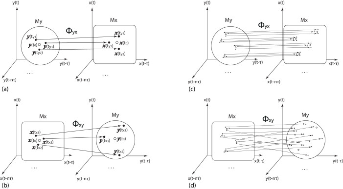
To begin, we revisit the mutual cross map method based on state space reconstruction. Consider two scalar time series x(t) and y(t) measured from two variables x and y in an unknown nonlinear dynamical system. With appropriately chosen embedding dimension L and proper delay τ24,25, one can obtain time delayed coordinate vectors x(t) = [x(t), x(t − τ), …, x(t − (L − 1)τ)]T and y(t) = [y(t), y(t − τ), …, y(t − (L − 1)τ)]T respectively. According to delayed embedding theory22, the set of vectors x(t) forms the reconstructed attractor Mx, and one can define My in an analogous way. For each point y(t0) on My, one can find its k nearest neighbors y(ty1), y(ty2), …, y(tyk) with time indices ty1, ty2, …, tyk. Moreover, one can define the mutual neighbors for x(t0) ∈ Mx as x(ty1), x(ty2), …, x(tyk) and the map from nearest neighbors to mutual neighbors is defined as cross map Φyx: My → Mx. In the case that x is causally influencing y, or x is a driving factor of y (i.e., x → y), the information of x is included in the dynamics of y, and thus two close states on My correspond to two close states on Mx, or explicitly, the mutual neighbors of x(t0) are also in the neighborhood of x(t0). Inversely, in the case that y has no influence over x, the dynamics of x is insensitive to the state of y and the mutual neighbors of y(t0) are not necessarily to be close to y(t0), as illustrated in Figs. 1(a) and (b). Therefore, the geometry property of mutual neighbors can be used to detect causality2,10,11. The details of mutual neighbors and cross map are revisited in Supplementary Information.
Figure 1. Illustration of mutual neighbors, cross map and smoothness.
(a) For one point y(t0) ∈ My and its counterpart x(t0) ∈ Mx, one can find the nearest neighbors  ,
,  ,
,  for y(t0) and define the mutual neighbors
  ,
,  ,
,  for x(t0). The map between the nearest neighbors and mutual neighbors is defined as cross map Φyx. In the case x causally influences y, the cross map Φyx maps a neighborhood to a neighborhood. (b) In the case y does not causally influence x, the cross map Φxy does not necessarily map a neighborhood to a neighborhood. (c) and (d) The global smoothness of Φyx and Φxy built from local smoothness.
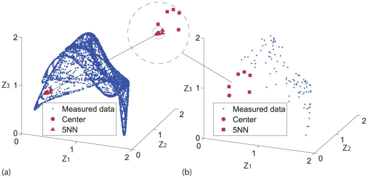
Here, it should be stressed that one requirement is essential, that is, the nearest neighbors for both x and y are required to be sufficiently close to the true neighborhood so that the local geometric information can be correctly measured. If this requirement is not fulfilled, contradictory results may be derived, e.g., the studies of refs. 10 and 11 used different assumptions for mutual predictions which both gave the same result. In fact, due to the computational way of state space reconstruction using delayed embedding technique, sufficiently long time series are required to guarantee that the nearest neighbors on the reconstructed attractor converge to the true neighborhood. Figure 2 shows the relationship between nearest neighbors and the time series length, where the nearest neighbors found on the attractor reconstructed from short time series (Fig. 2(b)) are apparently far away from the true neighborhood of the underlying center point (Fig. 2(a)). Detailed discussions and explanations on the necessity of convergence of nearest neighbors can be further referred to ref. 2. Thus, detecting causality based on nearest neighbors and mutual neighbors essentially requires sufficiently long time series data to make reliable causality detection.
Figure 2. Illustration for the time series length and convergence of nearest neighbors.
Here the time series are generated by one chaotic Lotka-Volterra system. (a) A reconstructed attractor from time series of 7000 samples, and the 5 nearest neighbors (5NN) of one center point. (b) A reconstructed attractor from time series of only 100 sampled points and the 5 nearest neighbors of the same center point. Inset: the comparison of the 5 nearest neighbors for both (a) and (b), where the latter set of points are apparently not close to the center point at all.
Here, we notice that the key idea behind the method of finding mutual neighbors is actually measuring the smoothness of the map. Specifically, if x causally influences y, the nearest neighbors of y(t0) are mapped to close states of x(t0), i.e., the cross map Φyx: My → Mx maps the neighborhood of y(t0) to the neighborhood of x(t0), which actually implies that Φyx is locally smooth around y(t0), as shown in Fig. 1(a). On the reverse direction, if y has no influence over x, the image of x(t0)'s neighborhood under the cross map Φxy: Mx → My is not necessarily the neighborhood of y(t0), thus the cross map Φxy is not necessarily smooth around x(t0), as shown in Fig. 1(b). If the cross map Φ is locally smooth in the neighborhood of every point on the attractor, then the map is globally smooth on the whole attractor, and vice versa. Thus, the global smoothness of Φyx and Φxy can be built from local properties, as illustrated in Figs. 1(c) and (d). Moreover, when the coupling strength increases, information becomes more distinct in the causally influenced variables. As a result, their attractors will contain stronger historical information from the causes. Thus, within one system, the relative smoothness can indicate the relative strength of causative effectiveness.
Therefore, finding mutual nearest neighbors is equivalent to measuring the smoothness of the cross map Φ, i.e., the smoothness of Φyx indicates the strength of causative effectiveness from x to y. While mutual neighbors only use the local information around one point, we propose a new framework, i.e., Cross Map Smoothness (CMS), to measure the smoothness of Φ using global information, and consequently we can detect causality even from short time series in an accurate manner. In other words, instead of finding nearest neighbors which requires a large number of samples, we computationally evaluate the smoothness of the cross map by designing an efficient algorithm for the global attractor.
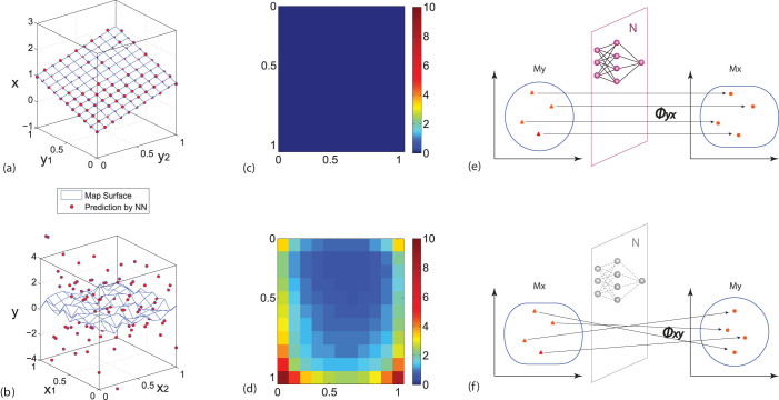
Our fundamental idea is based on the fact that any smooth map can be approximated by a neural network  26 while training a neural network to approximate an unsmooth map will fail with large training errors, as illustrated in Figs. 3(a)–(d). Furthermore, the training errors reflects the relative smoothness, and thus can be a measure of the relative strength of causative effectiveness. Therefore we can train the neural network
  to approximate the map Φyx, using the whole set of data y(t) on My as input and the whole set of data x(t) on Mx as output. Thus the training error (i.e., the measurement of the relative smoothness) between Φ and
  indicates the strength of the causative influence from x to y. The sketch of the Cross Map Smoothness (CMS) with the neural network (NN) method is illustrated in Figs. 3(e) and (f).
Figure 3. Sketch of the cross map smoothness learned by a neural network (NN).
(a) and (b) Illustrations for the neural network's approximation ability for smooth map and unsmooth map. Here the map surface in (a) is assumed to be x = y1 + y2 and the surface in (b) is simply generated by random points. (c) and (d) The prediction error (or the smoothness of Φ) for cases in (a) and (b) respectively, where the leave-one-out scheme is used to calculate errors. (e) Assume that x causally influences y, the information of x has been encoded in My and consequently Φ: My → Mx maps a neighborhood of y to a neighborhood of x, implying Φyx is smooth. Thus a neural network  can be trained to approximate the map based on the measured data on Mx and My. (f) Assume that y has no impact on x, then Mx has no information from y. Training a neural network to approximate the unsmooth map Φ: Mx → My will fail.
Thus, we propose the Cross Map Smoothness(CMS) algorithm using a Radial Basis Function (RBF) network to detect causality between two variables x and y. The details of the algorithm is listed in Supplementary Information Section 2. Here we adopt a leave-one-out strategy to fully use the short time series, i.e., we train one RBF network based on each leave-one-out data set and make prediction on the one test point. Finally, we compute the causality index Rxy based on the the normalized training error, which measures the causative effective strength from x to y.
Results
To validate the method, several representative examples are considered as benchmarks.
Theoretical model validation
Let us begin with several representative causality patterns which can be used as motifs in many complex situations. We first consider two coupled variables with both unidirectional and bidirectional couplings in the following form,
 |
where rx = 3.7 and ry = 3.8 are two coefficients. Here γxy and γyx are two coupling parameters and indicate the strength of causative effectiveness. In the first case, we set γxy = 0 and γyx = 0.32, which implies that X and Y have a driving-response relation, namely there is unidirectional causality from X to Y, while the inverse is not true. We use time series with length of 20 time points and apply the CMS method to the data set. The causality detection result obtained by CMS Algorithm is shown in Fig. 4(a), where nonzero Rxy and zero Ryx clearly fit with the unidirectional causality pattern. Then we set γyx = 0.1 and γxy = 0.02 which makes it a mutually coupled system, and thus there is mutual causative effectiveness between X and Y. With the same setting in the first case, we detect the causality between X and Y using CMS, as shown in Fig. 4(b). The detected result with Rxy = 0.69 and Ryx = 0.32 not only shows the bidirectional causality between X and Y but also indicates that the relative strength of the causative effectiveness from X to Y is stronger than the inverse direction.
Figure 4. Coupling relationship patterns (coupling strength γ in the left column) and the corresponding causality patterns (detected index R in the right column), where only the significantly detected causal relations above threshold are shown.
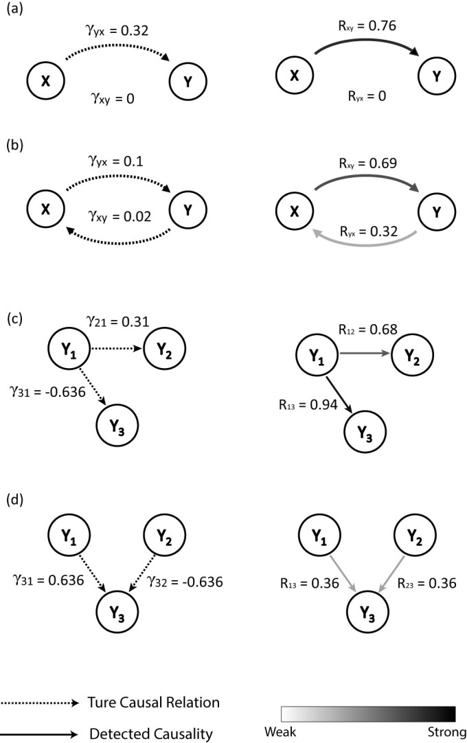
(a) Unidirectional causality pattern in the 2 species model. (b) Bidirectional causality pattern in the 2 species model. (c) Fan-out causality pattern. (d) Fan-in causality pattern.
Here it is stressed that within one system when all the other conditions are the same, as the coupling strength increases, information becomes more distinct in the causally influenced variables, and consequently larger causality indices will be detected. However, this strength of causative effectiveness is relative but not absolute, i.e., the relation is not always monotonous between the coupling parameter values and the coupling strength. Therefore, the detected index reflects the relative strength of the causative effectiveness between different pairs of variables within one system. To this end, we consider varying coupling strength values. In the unidirectional case, we fix γxy = 0 and vary the values of γyx in the range [0, 0.32]. For each value of γyx, we generate data and use the CMS algorithm to detect causal relations with the same setting. The result is shown in Fig. 5(a) where the detected Ryx is always zero while Rxy firstly jumps from zero to nonzero, then shows an ascending trend as the coupling strength increases. In the bidirectional case, we consider the following varying form: γyx = α, γxy = 0.2 − α where α is a varying factor in the range [0, 0.2] measuring the coupling strength in both directions. With the same setting as in the unidirectional case, the detected result is shown in Fig. 5(b) where zero causality indices reflect zero couplings and the detected causality indices Rxy and Ryx show ascending or descending trend as the coupling strength varies in the same way. Moreover, for small α, it clearly shows Ryx > Rxy which coincides with the fact of relative stronger causative effectiveness from X to Y, and vice versa.
Figure 5. Causality index detected for varying the coupling strength values.
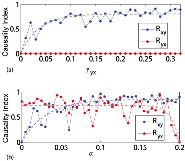
Dotted lines are the fitted trend curves. (a) Unidirectional case. (b) Bidirectional case.
Then we consider a more complicated system involving three variables as follows:
 |
where γij are coupling parameters. With particular settings of the coupling parameters, shown in Supplementary Information, the causal relations between the three variables can show fan-out or fan-in patterns, as shown in Figs. 4(c) and (d). For the fan-out case in Fig. 4(c), there are two unidirectional couplings from Y1 to Y2 and Y3, while Y2 and Y3 have no direct relationship with each other. Since Y2 and Y3 are both driven by the common source from Y1, the dynamics of Y2 and Y3 both contain the information from Y1. Thus the time series Y2(t) and Y3(t) are correlated but have no causality between them, which is a difficult situation for causality detection7. Here we apply the CMS method to the time series with length of 20 points, and get the mutual relationship between Y1, Y2 and Y3, which is shown in Fig. 4(c), where only the detected causality over significance threshold is shown. The result in Fig. 4(c) indicates that we can detect causality from Y1 to Y2 and Y3 but not vice versa. Furthermore, there is no causal relationship detected between Y2 and Y3, which confirms that our method is effective for common source causality pattern even with short-term data. As for the fan-in case in Fig. 4(d), there are two unidirectional couplings to Y3, i.e., Y3 is driven by both Y1 and Y2 simultaneously. With the same setting as the fan-out case, we use CMS to detect the mutual relationship between the three variables, as shown in Fig. 4(d). The result illustrates that we can correctly detect the fan-in causality pattern. Here we stress that the strength of the detected nonzero causality in Fig. 4(d) is much weaker than the previous cases. Actually, a fan-in motif is generally considered as a difficult pattern to infer17, this is mainly due to the fact that the dynamics of Y3 are affected by both Y1 and Y2 at the same time, which weakens the effect of each single driving force.
The above cases validate that our method can be effective for discrete-time dynamical systems. To test our method with continuous-time systems, we consider the Lorenz system driven by a chaotic signal from the Rössler system, which was used as a benchmark in ref. 11. We use the standard parameter values with which the coupled system has chaotic dynamics. We assume that 50 time points with an even measurement interval are observed from the systems and use CMS to detect the causality between the two systems. The detected causality indices are RLR = 0 and RRL = 0.27, which clearly shows the unidirectional causal relation from the Rössler system to the Lorenz system.
Here we note that though we use the normalized error in CMS Algorithm, the final causality index RYX for non-causal situation does not reach exactly zero. Therefore in order to decide whether the causality relation exists, we set a threshold value ξ based on the significance test18,27,28,29. Our statistical analysis is based on the permutation test: we run 1000 independent permutations uniformly at random, shuffle the time points according to the permutations, and run CMS on the shuffled data. With the empirical distribution, we estimate the threshold as ξ = 0.001 at a significance level p < 0.05, i.e., we treat a causality index below 0.001 as zero. The details of the significant test is shown in Supplementary Information.
The above illustrations show that our method is effective even for the situations where only short-term data can be obtained. On the other hand, in many occasions, owing to strong nonstationary and irregular behavior of many real-world systems, the causal relationship between system variables may switch quickly and thus even if a long time series is available the causality detected based on the long-term time series is meaningless. To consider such problems, we assume that the coupling parameters in system (1) are no longer constant but switching at random intervals between two sets of values so that the causal relationship between the two variables change from time to time, as shown in Fig. 6. We assume that a time series of 1000 time points are measured for the system, and it is obvious that using the whole time series to calculate one constant causality between X and Y will yield a false result. Therefore we use a time window of 20 time points moving along the whole time series and use the CMS method to detect causality from every short piece of data during one time window. Figure 6 shows the detected result, where the dashed square waves represent the random switching of the coupling parameters between zero and nonzero values and the solid lines represent the detected strengths of causative effectiveness over each time window. The switching value of γxy decides whether or not there is causative effectiveness from Y to X and it is clear that the detected causality from Y to X coincides with the square wave of γxy quite well in Fig. 6(a). The similar result can be observed for the causality from X to Y and the switching values of γyx in Fig. 6(b), which confirms the effectiveness of our method for such causality-varying situations.
Figure 6. Causality detection for a parameter-varying system in a piecewise manner.
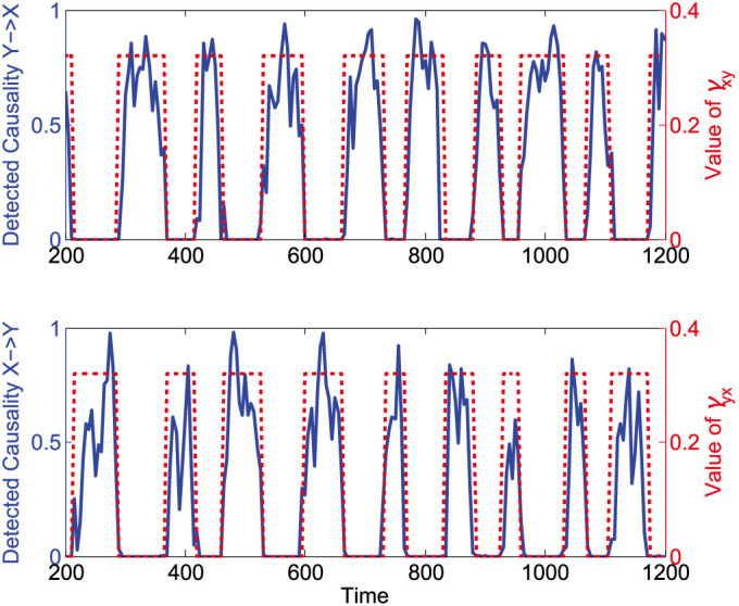
The dashed square waves represent the random switching of the coupling parameters between zero and nonzero values, and the solid lines represent the detected strengths of causative effectiveness over each time window.
Unraveling gene regulatory networks
How to infer gene regulatory interactions from transcriptomics time-resolved data, and further unravel the gene regulatory network (GRN) is of paramount importance to gain a deeper insight into the complexity and functions of the underlying biological systems. Due to the limit of experiment technique and other constraints, usually only very short-term and often noisy timeresolved measurements can be available in gene expressions. Though various methods based on Bayesian inference, regression analysis, econometrics models and standard similarity measures have been used to analyze such short time series data17,18,19, inferring genetic networks from short data is still regarded as an ‘ill-posed' inverse problem and a challenging task20,21.
Here, we note that in a gene regulatory network, the regulation mechanism obeys some biochemistry rules and thus the regulatory dynamics can be described by standard kinetics models, such as Michaelis-Menten and Hill kinetics30,31. Therefore, the regulatory interactions can be measured by causal relationship in nonlinear dynamical systems and the proposed CMS method can be particularly suitable for such a task, i.e., reverse engineering GRN from short-term data.
Since in the real time-resolved expression data, e.g., microarray chip data, not every regulatory subnetwork contains information of all the participating genes, particularly over a specific time period and a specific condition of interest. These facts render it challenging to give a comprehensive evaluation of network inference with real time-resolved expression data. On the other hand, it is widely accepted these years to evaluate inference methods using standard synthetically generated data sets17,18,19. Therefore, before applying our method with real data, we give a comprehensive validation with synthetically generated data sets of the bacterium E. coli30, as described in ref. 32.
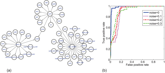
Specifically, we consider a subsystem consisting of 50 genes picked out randomly from the whole network, whose regulatory relation is shown in Fig. 7(a). The regulation network of the selected subsystem consists of several clusters, as illustrated in Fig. 7(a), which can well approximate the statistical properties of the whole network30. Here each node's dynamics is governed by Michaelis-Menten or Hill kinetics, so that the simulated gene expression time series are similar to real microarray measurements. We assume that only 10 time points are available for each gene expression time series to simulate the real experimental measurements and use CMS to detect causality between each pair of genes. In order to evaluate the inference efficiency of CMS to detect GRN structure, we use the resulting receiver operating characteristics (ROC) curves, which plot the true positive rate (TPR) against the false positive rate (FPR) at various threshold settings. Actually, ROC curves show the relative trade-offs between benefits of correctly inferred links (TPR) and the drawbacks of incorrectly inferred links (FPR) with different values of threshold to identify a link. The ROC curve for noise-free data is shown in Fig. 7(b), from which it can be concluded that the ROC curve is very close to the perfect classification; i.e., when FPR is controlled to be less than 2.5%, TPR can reach more than 90%, and the area under curve (AUC) is 0.98 which is very close to be one. Therefore, the CMS method can achieve a very good result for noise-free data. Meanwhile, generally noise-free expression data cannot be obtained in real experiment, and thus we need to further test the robustness of the method to include various kinds of noise in the time series. Here we consider three kinds of noise simultaneously, namely, the biological noise, the experimental noise and noise on correlated inputs with three different noise intensities, namely 0.1, 0.2 and 0.3. Figure 7(b) shows the three ROC curves for data with noisy perturbations, where we can conclude that though the ROC curves for noisy data are lower than the ROC curve for noise-free data, the accuracy is still very high; especially all the three ROC curves have AUC values around 0.9.
Figure 7.
(a) Regulatory network with the selected 50 genes of E. coli. (b) The ROC curves of the detection results by our method (CMS), with different levels of the noise condition.
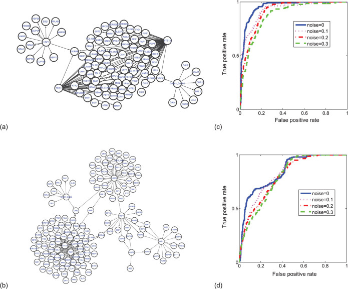
Moreover, to consider the influences of network properties such as size and degree, we further test two additional data sets for S.cerevisiae with 100 and 150 genes respectively. The selected subsystems are shown in Figs. 8(a) and (b), and based on 10 output of the gene expressions, we apply CMS to infer the network interactions respectively. The ROC curves for both non-noise and noise disturbed cases are given in Figs. 8(c) and (d). Here, it is noticed that there are two central genes which regulate other downstream genes at the same time for the selected subnetworks of S.cerevisiae, which makes fan-in and fan-out motifs abundant. As discussed in Figs. 4(c) and (d), the fan-in motif may lead the causality less significant to be detected, making it more difficult to detect the true network.
Figure 8.
(a) Regulatory network with the selected 100 genes of S.cerevisiae. (b) Regulatory network with the selected 150 genes of S.cerevisiae. (c) The ROC curves of the results for the network in (a) by our method, with different levels of the noise condition. (d) The ROC curves of the results for the network in (b) by our method, with different levels of the noise condition.
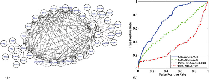
Next, we test our method with real gene expression data. Here we consider the data of the laboratory rat (Rattus norvegicus) cultured cells sampled from suprachiasmatic nucleus (SCN) for studying circadian rhythm, where the gene expression profiles are measured with Affimetrix microarray (Genechip Rat Genome 230 2.0)33,34,35. To elucidate the gene regulation network architecture, we select the data set consisting of 16 measured time points after the drug perturbation in the 19th hour. For the mammalian circadian clocks, it has been identified that there are around 17 genes involved in the core regulation network, where the transcriptional circuits are formed by regulation of E/E′ boxes, DBP/E4BP4 binding elements and RevErbA/ROR binding elements respectively36,37. Moreover, besides the gene-level interactions, there are also regulation interactions at the protein level; e.g., the transcription factor Clock is phosphorylated by PFK family genes and the crytochrome genes Cry1 and Cry2 are phosphorylated by MAPK family genes33. Therefore, we consider the 17 core circadian genes as well as 18 kinase genes, whose relations are depicted in Fig. 9(a). With 16 time points measured for each gene's expression, we apply the CMS method to detect the regulation relation between all the selected 35 genes. As a comparison, we also apply IOTA, partial IOTA18 and CCM2 to the same data set, where IOTA is a newly proposed permutation-based asymmetric association measure to detect regulatory links from very short time series and CCM is a mutual cross map-based method. Based on the core regulation network in ref. 36, we carry out the ROC analysis for the regulation detection, and the results are shown in Fig. 9(b).
Figure 9.
(a) Regulatory network with the selected circadian genes, where the solid lines indicate gene-level regulations and the dashed lines imply protein-level interactions. (b) The ROC curves of the results, with four methods tested on the same data set.
Here, we stress that inference of GRN based on only one single short-term data set is a challenging task due to the extremely short measurements. The existing methods for GRN inference can usually reach an AUC around 0.7 for synthetical data but only around 0.5 for real experimental data21. The CCM method, which relies on finding nearest neighbors and thus requires long-term data for the convergence, has AUC around 0.5 in Fig. 9(b). Particularly, the core transcriptional circuits of mammalian circadian clocks consist of complexly integrated regulatory loops involving three kinds of middle elements: E/E′ boxes, DBP/E4BP4 binding elements and RevErbA/ROR binding elements. Therefore in the circadian data set we used here, there are many fan-in motifs and the relation between two interacting subsystems may no longer be monotonic, and thus the IOTA method and the partial IOTA method may lead to a false result, as shown in Fig. 9(b) where the AUC of the IOTA method is less than 0.5.
As shown for the both synthetical GRN data and the real GRN data, our CMS method which is particularly effective for short-term data can achieve a very good result in a much accurate way in ROC analysis.
Discussion
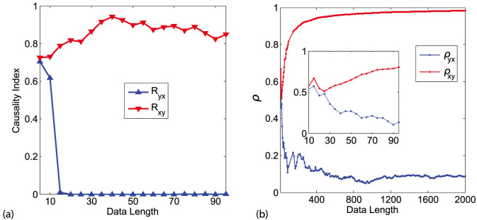
In this section, we discuss several issues related to CMS' application in real situations. First a question arises naturally: how short can be the time series so that CMS can be effective? Or explicitly, what is the lower bound of the length of time series that CMS requires to guarantee a reliable result. Intuitively, the longer the time series can be observed, the more information the data can provide. Therefore just as pointed out in ref. 2, one should consider the convergence of the causality index over different lengths of time series and use the limit value as the truly detected causality index. Here we use system (1) with unidirectional causality setting as a benchmark to test the lower bound for the CMS method. The result is shown in Fig. 10(a), which indicates that with around 20 time points, it is enough for CMS to distinguish zero and nonzero causality. Meanwhile, as a comparison, we also test the CCM2 method for the same data set. Since the CCM uses the convergence of nearest neighbors to detect causality, it needs much longer data length to converge. As shown in Fig. 10(b) as well as the inset there, CCM cannot distinguish zero and nonzero causality with short length of data, and with as long as 2000 time points, CCM can give a trend of convergence for nonzero causality though still no convergence for zero causality is achieved. Therefore, we conclude that CMS method can be effective for short-term data with length n ~ O(10) while the existing neighborhood-based method requires data with length n ~ O(103) to reach a reasonable result.
Figure 10.
(a) The causality detected by CMS based on different lengths of time series. (b) The causality detected by CCM based on different lengths of time series, where the inset is the enlarged part for the same data length as in (a).
Then we compare our method with some representative existing methods for causality detection. Here we choose two kinds of methods for comparison, namely, the mutual cross map based on nearest neighbors and the composition alignment method. For the former, we use the newly proposed CCM2 and for the latter, we use IOTA which is purposely designed for inferring gene networks from short time series18. We test all the numerical results in our paper with the same condition for the two methods, and the comparison results for the theoretical models are shown in Fig. 11. Moreover, for the gene networks, we consider several criteria to compare the methods, i.e., we consider the area under the ROC curve (AUC(ROC)), the Youden index (YOUDEN = max(the true positive rate - the false positive rate)), and the area under the Precision/Recall curve (AUC(PvsR)) which is based on the comparison between the true edges and the inferred ones. The results for these ROC analysis are shown in Table 1. Generally, it is suggested that a method has an excellent performance if conditions AUC(ROC) > 0.8; YOUDEN > 0.5 and AUC(PvsR) > 0.05 are satisfied simultaneously19. We highlighted the scores with the excellent performances in Table 1. Clearly, we see that CMS performs well in all the three cases. Since CCM needs long term data for convergence, the accuracy of results by CCM based on short term data here is poor. As for IOTA, it is specifically designed for gene network inference, and one crucial point of the IOTA approach lies on the assumption that two interacting genes have monotonic relationship. Therefore, for a general nonlinear dynamical system or gene expression which does not obey the monotonic assumption, the IOTA method may fail.
Figure 11. Comparison results for three methods on theoretical models.
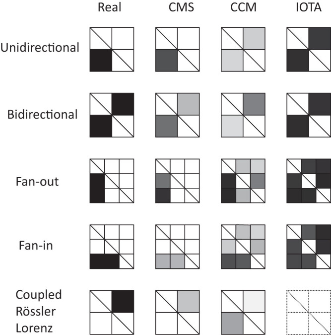
The left column shows the causality patterns in 5 models, where black blocks shows causality from vertical variables to horizonal variables. The gray scale represents the strength of the detected causality between 0 (white) and 1 (black).
Table 1. Comparison results for three method on four GRN cases, where three criteria are listed and the scores with the excellent performances are highlighted.
| AUC(ROC) | YOUDEN | AUC(PvsR) | |||||||
|---|---|---|---|---|---|---|---|---|---|
| CMS | CCM | IOTA | CMS | CCM | IOTA | CMS | CCM | IOTA | |
| Ecoli50 | 0.98 | 0.43 | 0.88 | 0.93 | 0.15 | 0.67 | 0.45 | 0.02 | 0.16 |
| Yeast100 | 0.95 | 0.68 | 0.75 | 0.79 | 0.51 | 0.5 | 0.18 | 0.02 | 0.17 |
| Yeast150 | 0.84 | 0.59 | 0.74 | 0.53 | 0.28 | 0.51 | 0.05 | 0.01 | 0.12 |
| SCN | 0.74 | 0.53 | 0.37 | 0.38 | 0.13 | 0.03 | 0.25 | 0.14 | 0.09 |
The above comparison results also imply that Rxy designed in CMS Algorithm can indicate the relative probability or the strength of causality taking values between 0 and 1. Therefore, we can use the CMS index R to detect whether there is causality and how strong the causal relation is between two variables, as shown in the gray scale used in Fig. 4 and Fig. 11. Note that though the CMS method uses the prediction error to measure causality, it is different from the measurement of the Granger method which uses a series y(t) to predict y(t) by constructing x(t) → y(t) correlation; our method uses a series y(t) to predict x(t) by constructing a y(t) → x(t) map, for inferring the causality from x(t) to y(t). It is also noted that the prediction error based methods cannot detect autoregulation, i.e., the causal effect from one variable to itself.
In conclusion, based on the state space reconstruction theory for nonlinear dynamics, we have developed a new method of CMS to detect causality between variables, even with short observed time series. The key idea of our method is to detect causative effectiveness by measuring the smoothness of the cross map between two observed variables rather than finding the nearest neighbors, thereby avoiding the requirement of long-term time series data. The method is validated with both theoretical benchmark models and real-world data from gene networks. Our method is particularly effective in situations where only short-term data are available, such as high throughput biological data. In this paper we adopted a neural network model to train a smooth map, and other methods constructing a smooth map can be also used in a similar way. As a future topic, we will consider to extend this method further to detect the causal relations of the measured variables just before the critical transitions38,39,40 and high dimensional measured variables of nonlinear dynamics41.
Supplementary Material
Supplementary Information for Detecting Causality from Nonlinear Dynamics with Short-term Time Series
Acknowledgments
We thank Prof. Hajimi Tei on the gene expression data and prior information collection. This research was supported by the Aihara Project, the FIRST program from JSPS, initiated by CSTP. This work was also supported by the NSFC (Nos. 61134013, 91029301, 61072149, 11301366, and 11326035), the Knowledge Innovation Program of CAS (No. KSCX2-EW-R-01), and 863 project (No. 2012AA020406).
Footnotes
The authors declare no competing financial interests.
Author Contributions H.M., L.C. and K.A. conceived the research; H.M. and L.C. performed the experiments, analyzed the data, and prepared the figures; All the authors wrote the manuscript.
References
- Granger C. W. J. Investigating causal relations by econometric models and cross-spectral methods. Econometrica 37, 424–438 (1969). [Google Scholar]
- Sugihara G. et al. Detecting causality in complex ecosystems. Science 338, 496–500 (2012). [DOI] [PubMed] [Google Scholar]
- Haufe S., Nikulin V. V., Mller K.-R. & Nolte G. A critical assessment of connectivity measures for EEG data: A simulation study. NeuroImage 64, 120–133 (2013). [DOI] [PubMed] [Google Scholar]
- Schreiber T. Measuring information transfer. Phys. Rev. Lett. 85, 461 (2000). [DOI] [PubMed] [Google Scholar]
- Paluš M., Komárek V., Hrnčíř Z. & Štěrbová K. Synchronization as adjustment of information rates: detection from bivariate time series. Phys. Rev. E 63, 046211 (2001). [DOI] [PubMed] [Google Scholar]
- Feldhoff J. H., Donner R. V., Donges J. F., Marwan N. & Kurths J. Geometric detection of coupling directions by means of inter-system recurrence networks. Phys. Lett. A 376, 3504–3513 (2012). [Google Scholar]
- Hirata Y. & Aihara K. Identifying hidden common causes from bivariate time series: a method using recurrence plots. Phys. Rev. E 81, 016203 (2010). [DOI] [PubMed] [Google Scholar]
- Chen Y., Rangarajan G., Feng J. & Ding M. Analyzing multiple nonlinear time series with extended Granger causality. Phys. Lett. A 324, 26–35 (2004). [Google Scholar]
- Ancona N., Marinazzo D. & Stramaglia S. Radial basis function approach to nonlinear Granger causality of time series. Phys. Rev. E 70, 056221 (2004). [DOI] [PubMed] [Google Scholar]
- Schiff S. J., So P., Chang T., Burke R. E. & Sauer T. Detecting dynamical interdependence and generalized synchrony through mutual prediction in a neural ensemble. Phys. Rev. E 54, 6708 (1996). [DOI] [PubMed] [Google Scholar]
- Quyen M. L. V., Martinerie J., Adam C. & Varela F. J. Nonlinear analyses of interictal EEG map the brain interdependences in human focal epilepsy. Physica D 127, 250–266 (1999). [Google Scholar]
- Hlaváčková-Schindler K., Paluš M., Vejmelka M. & Bhattacharya J. Causality detection based on information-theoretic approaches in time series analysis. Phys. Rep. 441, 1–46 (2007). [Google Scholar]
- Chicharro D. & Andrzejak R. G. Reliable detection of directional couplings using rank statistics. Phys. Rev. E 80, 026217 (2009). [DOI] [PubMed] [Google Scholar]
- Arnhold J., Grassberger P., Lehnertz K. & Elger C. A robust method for detecting interdependences: application to intracranially recorded EEG. Physica D 134, 419–430 (1999). [Google Scholar]
- Deyle E. R. et al. Predicting climate effects on Pacific sardine. Proc. Nat. Acad. Sci. USA 110, 6430–6435 (2013). [DOI] [PMC free article] [PubMed] [Google Scholar]
- Wang Y., Joshi T., Zhang X. & Chen L. Inferring gene regulatory networks from multiple microarray datasets. Bioinformatics 22, 2413–2420 (2006). [DOI] [PubMed] [Google Scholar]
- Marbach D. et al. Revealing strengths and weaknesses of methods for gene network inference. Proc. Nat. Acad. Sci. USA 107, 6286–6291 (2010). [DOI] [PMC free article] [PubMed] [Google Scholar]
- Hempel S., Koseska A., Kurths J. & Nikoloski Z. Inner composition alignment for inferring directed networks from short time series. Phys. Rev. Lett. 107, 054101 (2011). [DOI] [PubMed] [Google Scholar]
- Hempel S., Koseska A., Nikoloski Z. & Kurths J. Unraveling gene regulatory networks from time-resolved gene expression data–a measures comparison study. BMC bioinformatics 12, 292 (2011). [DOI] [PMC free article] [PubMed] [Google Scholar]
- Wang X., Wu M., Li Z. & Chan C. Short time-series microarray analysis: Methods and challenges. BMC Systems Biology 2, 58 (2008). [DOI] [PMC free article] [PubMed] [Google Scholar]
- Wang M. et al. LegumeGRN: A Gene Regulatory Network Prediction Server for Functional and Comparative Studies. PloS one 8, e67434 (2013). [DOI] [PMC free article] [PubMed] [Google Scholar]
- Takens F. Dynamical Systems and Turbulence Rand, D. A. & Young, L. S. (ed.) 366–381 (Springer-Verlag, New York, 1981). [Google Scholar]
- Sauer T., Yorke J. A. & Casdagli M. Embedology. Journal of statistical Physics 65, 579–616 (1991). [Google Scholar]
- Kantz H. & Schreiber T. Nonlinear time series analysis (Cambridge University press, Cambridge, 2004). [Google Scholar]
- Kennel M. B. et al. Determining embedding dimension for phase-space reconstruction using a geometrical construction. Phys. Rev. A 45, 3403–3411 (1992). [DOI] [PubMed] [Google Scholar]
- Park J. & Sandberg I. W. Universal approximation using radial-basis-function networks. Neural Comput. 3, 246–257 (1991). [DOI] [PubMed] [Google Scholar]
- Nichols T. E. & Holmes A. P. Nonparametric permutation tests for functional neuroimaging: A primer with examples. Hum. Brain Mapp. 15, 1–25 (2002). [DOI] [PMC free article] [PubMed] [Google Scholar]
- Luo Q., Ge T. & Feng J. Granger causality with signal-dependent noise. Neuroimage 57, 1422–1429 (2011). [DOI] [PubMed] [Google Scholar]
- Guo S. et al. Uncovering interactions in the frequency domain. Plos. Comput. Bio. 4, e1000087 (2008). [DOI] [PMC free article] [PubMed] [Google Scholar]
- Van den Bulcke T. et al. SynTReN: a generator of synthetic gene expression data for design and analysis of structure learning algorithms. BMC bioinformatics 7, 43 (2006). [DOI] [PMC free article] [PubMed] [Google Scholar]
- Hofmeyr J.-H. S. & Cornish-Bowden H. The reversible Hill equation: how to incorporate cooperative enzymes into metabolic models. Comput. Appl. Biosci. 13, 377–385 (1997). [DOI] [PubMed] [Google Scholar]
- Shen-Orr S. S., Milo R., Mangan S. & Alon U. Network motifs in the transcriptional regulation network of Escherichia coli. Nat. Genet. 31, 64–68 (2002). [DOI] [PubMed] [Google Scholar]
- Wang Y., Zhang X.-S. & Chen L. A network biology study on circadian rhythm by integrating various omics data. OMICS 13, 313–324 (2009). [DOI] [PubMed] [Google Scholar]
- Kawaguchi S. et al. Establishment of cell lines derived from the rat suprachiasmatic nucleus. Biochem. Bioph. Res. Co. 355, 555–561 (2007). [DOI] [PubMed] [Google Scholar]
- Morioka R. et al. Phase Shifts of Circadian Transcripts in Rat Suprachiasmatic Nucleus. In The Second International Symposium on Optimization and Systems Biology. 109C114 (World Publishing Corporation, Lijiang, China, 2008). [Google Scholar]
- Ueda H. R. et al. System-level identification of transcriptional circuits underlying mammalian circadian clocks. Nat. Genet. 37, 187–192 (2005). [DOI] [PubMed] [Google Scholar]
- Ko C. H. & Takahashi J. S. Molecular components of the mammalian circadian clock. Hum. Mol. Genet. 15, R271–R277 (2006). [DOI] [PubMed] [Google Scholar]
- Chen L. et al. Detecting early-warning signals for sudden deterioration of complex diseases by dynamical network biomarkers. Sci. Rep. 2, 342 (2012). [DOI] [PMC free article] [PubMed] [Google Scholar]
- Liu R. et al. Early diagnosis of complex diseases by molecular biomarkers, network biomarkers, and dynamical network biomarkers. Medicinal Research Reviews 34, 455–478 (2013). [DOI] [PubMed] [Google Scholar]
- Liu R. et al. Identifying critical transitions of complex diseases based on a single sample. Bioinformatics 30, 1579–1586 (2014). [DOI] [PubMed] [Google Scholar]
- Ma H. et al. Predicting Time-Series from Short-Term High-Dimensional Data. Int. J. Bifurcat. Chaos 24, 1430033 (2014). [Google Scholar]
Associated Data
This section collects any data citations, data availability statements, or supplementary materials included in this article.
Supplementary Materials
Supplementary Information for Detecting Causality from Nonlinear Dynamics with Short-term Time Series


