Metabolic modeling of dynamic ¹³C NMR isotopomer data in the brain in vivo: Fast screening of metabolic models using automated generation of differential equations

Abstract

Most current brain metabolic models are not capable of taking into account the dynamic isotopomer information available from fine structure multiplets in ¹³C spectra, due to the difficulty of implementing such models. Here we present a new approach that allows automatic implementation of multi-compartment metabolic models capable of fitting any number of ¹³C isotopomer curves in the brain. The new automated approach also makes it possible to quickly modify and test new models to best describe the experimental data. We demonstrate the power of the new approach by testing the effect of adding separate pyruvate pools in astrocytes and neurons, and adding a vesicular neuronal glutamate pool. Including both changes reduced the global fit residual by half and pointed to dilution of label prior to entry into the astrocytic TCA cycle as the main source of glutamine dilution. The glutamate-glutamine cycle rate was particularly sensitive to changes in the model.

Introduction

Metabolic modeling of ¹³C labeling curves during infusion of ¹³C-labeled substrates allows determination of metabolic rates in the brain [1], [2]. In recent years, it became possible to measure not only total enrichment curves at individual carbon positions (e.g. C2, C3, C4 of glutamate), but also labeling curves for individual isotopomers, which appear as fine structure multiplets in ¹³C spectra [3–6]. This additional information can potentially be used to improve the accuracy and precision of fitted metabolic rates [7]. In addition, it is more likely to reveal discrepancies between the data and the best fits, and the metabolic model can then be improved in order to better match the experimental data.

However, implementation of a metabolic model capable of fitting the additional isotopomer curves remains a challenge. Even using compact formulations such as bonded cumomers [7], metabolic models still consist in hundreds of variables and coupled differential equations. Not only is a human operator likely to introduce errors in such a large system of equations, but also the time required to manually write the equations makes it impossible to easily modify the biochemical network by introducing new metabolites or reactions. This prevents fast implementation and testing of small changes in the metabolic network, such as adding metabolic pools or reactions to better explain the data. Therefore, an automated approach is greatly needed.

A number of approaches have been proposed to automatically determine metabolic fluxes from the distribution of ¹³C isotopomers without having to manually write the equations [8–12]. These approaches are based on the description of elementary reactions, in terms of atom distribution matrix ADM or equivalents [8–10], or other [11], [12], which were used to numerically build the system of equations and solve it. To the best of our knowledge, only one previous study reported the derivation of analytical equations for isotopomers [13], but this was achieved for the steady-state (not dynamic) isotopomer balance, and using the symbolic toolbox of Matlab. None of the above-mentioned approaches, however, can be readily used to fit in vivo brain ¹³C isotopomer time courses.

In the present work, we introduce an algorithm allowing the automatic writing of cumomer differential equations and of the associated cost functions used to fit experimental data. Equations are written in text format, with the names of variables appearing explicitly, thus making them easy to read for a human operator. Moreover, the system of equations is automatically simplified by taking into account the specific substrate being infused and the specific metabolites being measured in order to retain only the minimum number of variables and equations necessary to fit the data.

We demonstrate the usefulness of the new method by fitting a large number of dynamic ¹³C isotopomer curves in the brain with various two-compartment neuronal-glial models. The new method permits quick changes in the metabolic network (in a matter of minutes) and assessment of the impact of these changes on the fit quality and the values of fitted metabolic rates.

1. Biochemical network analysis and generation of the differential equations

1.1. Representation of biochemical network

A biochemical network is composed of the metabolites involved in the network, and of the biochemical reactions between these metabolites. The network is connected to the “outside” by some influxes and effluxes.

Metabolites and cumomers

By definition, a cumulative isotopomer fraction (or cumomer fraction) for metabolite M, noted π_M{i}, (where {i} is a set of integers i₁, i₂…,i_n, indicating carbon positions), is the sum of isotopomer fractions for all isotopomers labeled at least at positions i₁, i₂…, i_n, whatever the label at other positions. The size n of the set {i} is the “order” of the cumomer [7].

The representation of a metabolite consists in its name and its carbon chain numeration. Then, a cumomer for this metabolite can be represented by a vector of integers, where the vector components represent the carbon positions being labeled. Cumomers of order n>3 are not considered since they do not contribute to the in vivo ¹³C spectra fine structure detectable in practice [7], so that only one, two or three integers define a cumomer. An important situation is the invariance of a metabolite stereo structure by a rotation or a succession of rotations, which leads to label scrambling. This is for example the case for succinate in TCA cycle. It is therefore crucial to systematically represent such invariance and to determine how label is scrambled. Briefly, the symmetry of the stereo structure creates equivalence between some cumomers, which can accordingly be regrouped in sets of equivalent cumomers [7]. A single cumomer can then be chosen within each set to represent all equivalent cumomers of this set.

Biochemical reactions

A biochemical reaction can be represented by a name, a flux value, the input metabolites (reactants) and output metabolites (products), and an atom distribution matrix (ADM) characterizing the biochemical reactions of the network [7], [14], [15]. The ADM describes how carbons are transferred between reactants and products. It lists the carbon positions for the reactants along its first dimension (rows), while it lists the carbon positions for products along its second dimension (columns), with coefficients 1 in the ADM indicating how the corresponding reactant’s carbon nucleus is transferred to the products.

Connection between the network and the “outside”: influxes and effluxes

Some metabolic pools in the network are connected to metabolic pools outside the network, which has to be taken into account by the model. Let’s consider a metabolite A inside the network, and the same metabolite A_O outside the network (for example, A can be the pool of cerebral glucose or lactate, and A_O can be the pool of plasma glucose or lactate). An influx from A_O to A at the rate V_in results in the synthesis of the cumomers π_A{k} at the rate [A]×(dπ_A{k})/dt=V_in×π_AO{k} where {k} is a set of integers indicating carbon positions. Hence an influx is characterized by the flux V_in and the values of the cumomer fractions for A_O. If the carbon chain of A_O is exactly labeled at positions {l}={l₁, l₂… l_M}, and {i} is the subset of {k} included in {l}, while the remaining p elements of {k} are not included in {l}, then π_AO{k}= π_AO{i}×0.011^p, due to the fact that natural abundance labeling (1.1%) can occur on the p carbons not specifically labeled. For example, assuming an infusion of [1,6–¹³C] glucose so that the glucose plasma (GLCpl) is enriched at 66%, then for 1^st order plasma glucose cumomers:

• π_GLCpl{1}=π_GLCpl{6}=0.66

• π_GLCpl{2}=… =π_GLCpl{5}=0.011

For 2^nd order cumomers:

• π_GLCpl{1,6}=0.66

• π_GLCpl{1,2}=… =π_GLCpl{5,6}=0.66×0.011

• π_GLCpl{2,3}=… =π_GLCpl{4,5}=0.011²

And for 3^rd order cumomers:

• π_GLCpl{1,2,6}=… =π_GLCpl{1,5,6}=0.66×0.011

• π_GLCpl{1,2,3}=… =π_GLCpl{4,5,6}=0.66×0.011²

• π_GLCpl{2,3,4}=π_GLCpl{2,3,5}=π_GLCpl{2,4,5}=π_GLCpl{3,4,5}=0.011³

In contrast, an efflux from a metabolite B (at rate V_eff) is a much simpler case: V_eff contribute to the decrease of π_B{k} according to the rate [B]×(dπ_B{k})/dt=−V_eff×π_B{k}, which is independent of a corresponding pool outside the network.

1.2. General algorithm for automatic generation of equations

The aim of the algorithm is to identify all sources of label inputs and outputs for all cumomers (see Figure 1. for a flowchart of the algorithm). The basic structure is the following: for all metabolites M and all π-functions (with order n≤3), all reactions of the network are looked through (note that if the metabolite is symmetric, only π-functions representing sets of equivalents are considered):

• –If the current reaction produces the considered metabolite M, the ADM is used to determine all the metabolites and associated π-functions required to produce the current π-function (and all its equivalents in the case of symmetric metabolites). The determination of source cumomers is done by looking, for each column of the ADM corresponding to the indices of the current π-function, the rows having nonzero terms. The position of these rows in the ADM yields the label sources and the corresponding cumomers, which contribute to the overall input at a rate V_reac, where V_reac is the current reaction flux. For cumomers of order higher than 1, the input function determined by the ADM can be a product of cumomers. For a produced cumomer of 2^nd order, if the two rows in the ADM representing the source of label stand for the p^th and q^th carbons of a single metabolite S1, then the input term is V_reac ×π_S1pq. Otherwise, the rows must belong to two different source metabolites S1 (p^th carbon) and S2 (q^th carbon), and the input term is V_reac×π_S1p×π_S2q. For a cumomer of 3^rd order, one can similarly have input terms of the form V_reac×π_S1pqr, V_reac×π_S1pq×π_S2r, or V_reac×π_S1p×π_S2q×π_S3r. Note that, if the produced metabolite M has symmetry of order N, the above input terms have to be divided by N [7]. Conversely, if one of the source metabolites S1, S2… is symmetric, its cumomers have to be replaced by the equivalent cumomers representing them.
• –If the current reaction uses M as a reactant, then the current reaction contributes to the overall efflux out of the current cumomer at the rate V_reac.

Figure 1.

Schematic of the algorithm analyzing the biochemical network and writing the system of differential equations.

Once all the network reactions have been examined, the effluxes and influxes between the network and the outside are considered as described in section 1.1.

Writing the set of differential equations is then done sequentially for each metabolite and each cumomer by concatenation of character strings.

1.3. Reducing the cumomer network for ¹³C NMR modeling

The algorithm presented above allows the determination of labeling time courses for all cumomers in the biochemical network. However, in the context of NMR spectroscopy, where only a few metabolites are detected and where label is injected in the network via a given set of substrates (for example [1,6–¹³C] glucose), some cumomers do not need to be taken into account. One can consider two different kinds of cumomers that do not need to be simulated:

• –Cumomers that remain constant (i.e. equal to 0.011ⁿ, where n is the order of the cumomer) throughout time, considering the actual label input in the network.
• –Cumomers that are independent of the “observed” cumomers (these “observed” cumomers are bonded cumomers corresponding to NMR detected metabolites [7]), i.e. which are never involved in the time-evolution of “observed” cumomers and of any of their precursors.

On the contrary, any cumomer that evolves through time and is involved at some point in the generation of an “observed” cumomer or one of its precursors has to be considered. Retaining only these cumomers and eliminating the others allows reducing the total size of the system without any loss of information regarding the final result, but with the benefit of reducing computational time and of making the system easier to read for the human eye.

The required cumomers are determined in two steps. First, an “ascending” analysis, starting from the observed cumomers, allows the recursive determination of all precursor cumomers. This yields the minimal list L_R of cumomers and equations required to describe the time-evolution of observed cumomers. Second, a “descending” analysis simulates the label flowing from a given set of substrates throughout the network, allowing the determination of cumomers that are actually not generated and remain constant for the considered set of substrates, which can consequently be eliminated from L_R as determined previously in the ascending analysis. The algorithm described in section 1.2 is then use to generate differential equations automatically. As a result, only differential equations for cumomers belonging to L_R are generated, the other cumomers being replaced by 0.011ⁿ whenever they appear as a source term on the right side of a differential equation. This yields a system with a reduced number of variables and equations that is sufficient to describe completely the NMR-detectable information for a given set of infused substrates.

The above algorithms were implemented in Matlab (The MathWorks, Inc., Natick, MA). Two equation files are generated: an explicit text file which can be understood by a human operator (with the metabolite names and carbon positions explicitly identified); and another in a format that can be used by Matlab routines for solving differential equation systems (such as ode15s), where all cumomers appear as the elements of a vector of cumomers y.

2. Fitting of in vivo data and fast screening of various metabolic models

Automatic generation of equations enables fast screening of metabolic models that would otherwise require a very lengthy and error-prone manual implementation, even for a simple modification such as adding a single metabolic pool. In this section, we demonstrate how this new tool can be used to quickly evaluate new metabolic models, starting with a two-compartment model currently used in the literature.

We tested four different models as described below. Each model was used to fit the same magnetic resonance spectroscopy (MRS) brain data acquired during continuous [1,6–¹³C₂] glucose infusion in rats [4]. The fitted data was the summed time course from 5 animals obtained under alpha-chloralose anesthesia. Each isotopomer curve was normalized by the mean of its last 4 points and scaled using information from spectra from brain extracts at the end point. More precisely, total carbon resonance curves were normalized using the fractional enrichment at the end point. Individual isotopomer curves within each multiplet were then scaled individually to match the relative contribution (area) of each component to that multiplet at the end point. Finally, those curves were converted to ¹³C concentrations curves by multiplying by 10 and 4 μmol/g for total glutamate and glutamine respectively [16], [17]. Glial glutamate was set to 1 μmol/g and the balance was split between neuronal and vesicular glutamate. After initial fitting with a model including vesicular glutamate (model 3), vesicular glutamate was set to 1.5 μmol/g, leaving 7.5 μmol/g for neuronal (cytoplasmic) glutamate (total glutamate = 10 μmol/g). Glutamine was separated between glia and neurons in a 1:7 ratio (i.e. neuronal glutamine = 0.57 μmol/g and glial glutamine = 3.43 μmol/g). The glucose input function was modeled as a linear function rising from 0 to 0.66 over the first minute of infusion and kept constant at 0.66 thereafter, closely matching the plasma glucose enrichment measured experimentally. The lactate input function was modeled as a linear function rising from 0 to 0.35 over 7 h, matching the value of plasma lactate enrichment measured experimentally at the end point after 7 h of glucose infusion. Furthermore, to minimize the introduction of bias by using isotopomer curves with low signal-to-noise, only curves with an end-point ¹³C concentration greater than 1.0 μmol/g were used. The fitted time courses were: Glu4Total, Glu4S, Glu4D34, Glu3Total, Glu3D, Glu3T, Glu2Total, Glu2S, Glu2D23, Gln4S, Gln4Total, Gln3Total, Gln2Total (13 curves). Fit quality was assessed using the mean squared error of the fit residuals for each individual curve as well as for all curves taken together. The precision for each flux was obtained by performing Monte-Carlo simulation over 500 draws. Random Gaussian noise was added to the initial fit of each curve. The noise level added to each curve was determined by performing a linear fit over the last quarter of the corresponding time course data and calculating the standard deviation of the residuals.

2.1. A traditional model used for ¹³C MRS data analysis: Model 1

The two-compartment model adapted from [18] (cf. Figure 2.) describes the sequential labeling of NMR visible glutamate and glutamine that can be separated between neuronal and astrocytic labeling. Both compartments contain a TCA cycle (V_TCA-A and -_N, for astrocytes and neurons respectively) and are linked via the glutamate-glutamine cycle exchange depicting neurotransmission (V_NT). An additional entry point of the astrocytic TCA cycle is the pyruvate carboxylase reaction (V_PC). The system uses a glucose influx distributed between neurons and astrocytes, an astrocytic glutamine efflux and a neuronal aspartate exchange with OAA (with aspartate assumed to be primarily neuronal). The exchange rate V_X between alpha-ketoglutarate and glutamate is assumed to be identical in both compartments. Supporting that assumption, we found that fitting separate V_X fluxes in neurons and astrocytes has minimal effect on fit quality (data not shown). A lactate dilution flux (Vdil_Lac) accounts for exchange of labeled lactated with lactate from the blood. An additional glutamine dilution (V_gln-dil) accounts for the lower enrichment in glutamine C4 relative to glutamate C4 [7].

Figure 2.

Two-compartment models tested in the present study. Model 1 included a single pyruvate/lactate pool (rectangular box) in exchange with the plasma lactate pool at a rate Vdil_Lac. This model is similar to those commonly used in the literature to fit dynamic ¹³C MRS data. In Model 2, the Pyr/Lac pool was divided into separate astrocytic and neuronal pools (grey boxes delineated by dotted lines) with separate dilution fluxes Vdil_LacA and Vdil_LacN respectively. Model 3 was identical to Model 1, but with addition of a vesicular glutamate pool (grey box delineated by dashed line). Model 4 combined both changes: addition of a glutamate pool and separate astrocytic and neuronal Pyr/Lac pools.

This model (Model 1) translates into a set of 266 equations and is reduced to 117 equations after ascending and descending analysis in the case of [1,6–¹³C₂] glucose infusion and detection of glutamate and glutamine C4, C3 and C2.

Best fits for glutamate and glutamine with Model 1 showed obvious discrepancies between the best fits and the data (Figure 3. and Figure 4., dotted lines). The GLU4Tot (total glutamate labeled at the C4 position) and GLU4S (glutamate C4 singlet) curves were largely underestimated in the latter part of the curves, and the GLU4D43 (glutamate C4 doublet) curve was imperfectly fitted as well (Figure 3. A, dotted lines). Best fits for glutamate C3 (Figure 3. B, dotted lines) closely approximated data, but small systematic deviations (∼ 0.2 μmol/g) were still noticeable. Similar to glutamate C4 curve, GLU2Tot and GLU2S curves were underestimated in the latter part of the time courses (Figure 3. C, dotted lines). Finally, the GLN4Tot curve was clearly overestimated (Figure 4. A, dotted lines), while the GLN2Tot and GLN3Tot curves were underestimated (Figure 4. B, dotted lines). Overall, such systematic deviations between the best fits and the data show that Model 1 is not accurate enough to account for the experimental data.

Figure 3.

Best fits of glutamate cumomer curves using Model 1 (dotted lines) and Model 4 (solid lines). A) Best fits of glutamate C4 curves B) Best fits of glutamate C3 curves and C) Best fits of glutamate C2 curves. Cumomer curves with a ¹³C concentration below 1 μmol/g (e.g. GLU3S, GLU2D21,…) were not fitted and are not shown.

Figure 4.

Best fits for total cumomer curves for glutamine in position C2 using Model 1 (dotted lines) and Model 4 (solid lines). A) Best fits of glutamine C4 curves and B) Best fits of glutamine C3 and C2 curves. Cumomer curves with a ¹³C concentration below 1 μmol/g were not fitted and are not shown.

The values of the seven fitted metabolic fluxes obtained with Model 1 are shown in Figure 5. (black bars). The neuronal TCA cycle rate V_TCA-N was 0.4 μmol/g/min and the astrocytic TCA cycle rate V_TCA-N was 0.2 μmol/g/min, or about 50% of V_TCA-N. V_X was about 2.5 μmol/g/min with a very high standard deviation, consistent with the high uncertainty on this flux reported in many studies. The pyruvate carboxylase flux was 0.05 μmol/g/min. V_NT was less than 0.02 μmol/g/min and both dilution fluxes (Vdil_Lac and V_gln-dil) were small. Those values are similar to those previously reported in the anesthetized rat brain under alpha-chloralose anesthesia, except for V_NT which was about ten-fold lower than previously reported values (range 0.18 – 0.27). [19]–[22]. Note, however, that the values of fitted metabolic fluxes obtained with Model 1 should be considered with some caution, given that the best fits showed large deviation from the experimental data.

Figure 5.

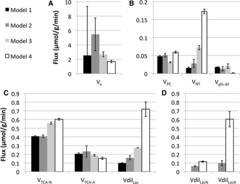
Estimated fluxes values obtained by fitting ¹³C MRS data acquired in rat brain under α-chloralose anesthesia with each of the four models. (A) value of V_X (B) Values of V_PC, V_NT and V_gln-dil. (C) Values of V_TCA-N, V_TCA-A and Vdil_Lac For Models 2 and 4, Vdil_Lac is the sum of Vdil_LacN and Vdil_LacA (total). (D) Values of Vdil_LacN and Vdil_LacA for Model 2 and Model 4. Adding a vesicular glutamate had a drastic effect on V_X estimation, giving a much lower value and reducing its uncertainty (Models 3 and 4). Addition of separate dilution fluxes in neurons and astrocytes yielded a much higher dilution in astrocytes than in neurons. In Model 4, most of the dilution occurred through lactate, with a very small residual glutamine dilution flux.

2.2. Separating glucose intake between neurons and astrocytes: Model 2

Model 1 assumes a single pyruvate/lactate pool with a single dilution flux Vdil_Lac. In Model 2, separate pyruvate/lactate pools are introduced for astrocytes and neurons, with separate dilution fluxes Vdil_LacA and Vdil_LacN, thus allowing different fractional enrichment in neurons and astrocytes, as reported in [21], [23], [24]. This second model can be described using a total of 119 equations after simplification.

There was no significant improvement in fit quality between Model 1 and Model 2, as indicated by the mean squared error of fit residuals (Figure 6.) (best fits not shown). The mean squared error was similar with both models, 0.65 (μmol/g)² with Model 1 and 0.67 (μmol/g)² for Model 2 (Figure 6.). Nonetheless, Model 2 gave a higher lactate dilution flux in astrocytes than in neurons (Figure 5. D, grey bars), consistent with previous results by Jeffrey et al [23] and consistent with astrocytes being located closer to blood vessels than neurons.

Figure 6.

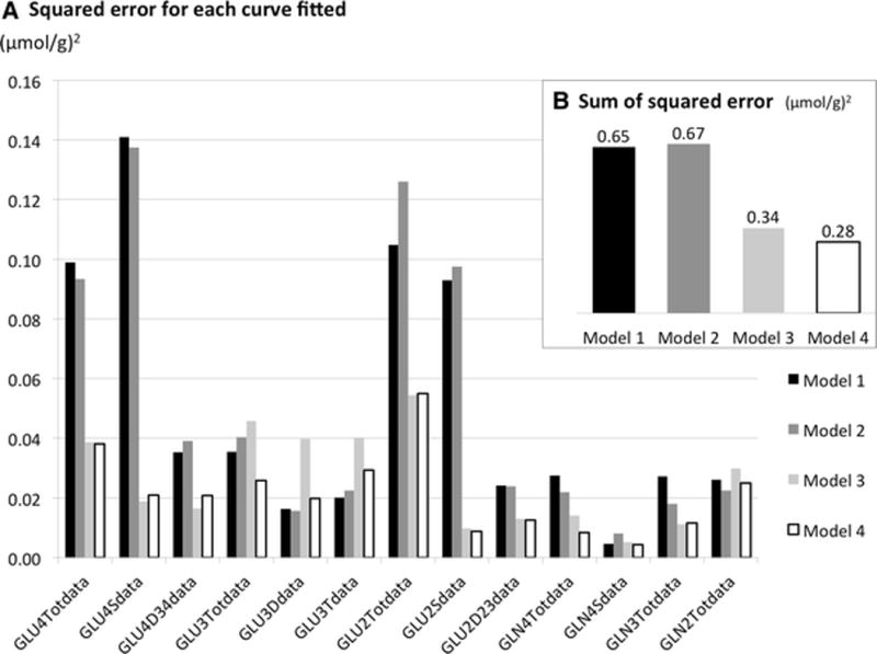
Mean squared error between data and best fit for each curve, in (μmol/g)². The square of the difference between experimental data and best fit was summed over the whole time-course, and divided by the number of time-points (N=73) to derive an error independent of the total time course duration.

2.3. Adding a vesicular glutamate pool: Model 3

Another biologically relevant modification to the model is the addition of a vesicular glutamate pool separate from the cytosolic glutamate pool. This addition led to a new set of 128 differential equations. The mean squared error for fit residuals showed that Model 3 resulted in a marked improvement in the fits of experimental curves compared to Models 1 and 2, especially for glutamate C4 and glutamate C2 curves, while the fits for glutamate C3 became worse (Figure 6., light grey bars vs. black bars).

Interestingly, simulations showed that the overshoot in the GLU4S curve was strongly dependent on the size of the vesicular glutamate pool (see Figure 7). As the size of the vesicular pool increases, the overshoot becomes less pronounced, consistent with labeling of part of the glutamate pool (the vesicular pool) being slightly delayed. When fitted as a free parameter, the vesicular glutamate pool size was estimated at 1.5 μmol/g. This value was subsequently used for both Model 3 and Model 4. The mean squared error for all fitted curves dropped by half from 0.65 to 0.34 (μmol/g)² when fitting with Model 3 compared to Model 1 (Figure 6. B).

Figure 7.

Effect of the size of the vesicular pool on the early time course overshoot observed in GLU4S and GLU2S isotopomer curves.

The estimated value and standard deviation for V_X were much lower with Model 3 than with Models 1 and 2, while the model returned a higher neurotransmission rate, higher pyruvate/lactate dilution and a greater difference between TCA cycle rates in neurons and astrocytes (Figure 5.).

2.4. Combining both changes: Model 4

Combining addition of vesicular glutamate and separate pyruvate pools in neurons and astrocytes resulted in Model 4, described by 130 differential equations. This model yielded the best fits of all four models (Figure 3. and Figure 4., solid lines) and the lowest overall mean squared error (0.28 (μmol/g)², Figure 6. B). It retained the improvements for the fits of GLU2 and GLU4 curves obtained with Model 3, while also mitigating the greater error for GLU3 introduced with that model (Figure 6. A, white bars). Best fits for glutamate C4 curves with Model 4 were excellent (Figure 3. A, solid lines), with only very small overestimation of the early part the GLU4D43 curve and very small underestimation of the GLU4S curve. Best fits for GLU2 curves (Figure 3. C, solid lines) and for glutamine (Figure 4., solid lines) were also very good and much improved compared to Model 1. Best fits for glutamate C3 were acceptable, although small systematic deviations from the data (on the order of 0.2 μmol/g) were apparent for all three curves (Glu3Tot, Glu3S, Glu3D43) (Figure 3. B, solid lines).

Looking at the values of fitted metabolic fluxes (Figure 5., white bars), the neuronal TCA cycle rate was larger with Model 4 (0.6 μmol/g/min) than with Model 1 (0.4 μmol/g/min), while the astrocytic TCA cycle rate was lower (0.15 vs 0.2 μmol/g/min), resulting in a higher V_TCA-N / V_TCA-A ratio (4:1 vs 2:1). The neurotransmission rate V_NT was 10-fold higher with Model 4 than Model 1 (Figure 5. B), illustrating the large sensitivity of this flux to changes in the metabolic network [18]. Overall lactate dilution was much increased with Model 4 compared to Model 1 (Figure 5. C), and lactate dilution was again higher in astrocytes than in neurons (Figure 5. D). In contrast, the glutamine dilution flux was much lower than with Model 1. Finally the V_X flux had a much lower value and better precision than with Model 1 (Figure 5. A).

3. Discussion

The new approach presented here allows quick implementation of any two-compartment model (or even models with more compartments) to fit any number of ¹³C NMR isotopomer curves simultaneously. With this approach, modifications in the metabolic model can be implemented in a matter of minutes. This is significant because of implementation of complex multi-compartment brain models capable of fitting ¹³C isotopomer curves has been the main roadblock to fitting such data and harnessing the additional information available from them. Largely because of this obstacle, only one previous study has reported fitting of isotopomer curves in the brain [23]. Moreover, in that study, only two isotopomer curves were fitted (GLU4S and GLU4D43), again because of the difficulty of implementing a model capable of fitting more curves.

Compared with manual implementation, the ability to automatically derive the equations not only saves a lot of time, but also greatly reduces the risk of error. The versatility of the algorithm also permits implementation of different infusion protocols, such as simultaneous infusion of [1,2–¹³C₂] acetate and [1,6–¹³C₂] glucose [5]. Finally, for the models used in this study, the automatic reduction in the number of equations (by eliminating equations for cumomers not labeled or not contributing to the measured signals) resulted in a 4-fold decrease in the execution time, which is particularly beneficial for Monte-Carlo simulations.

The more curves are fitted, the more information is available to the model, which provides more experimental constraints for the fit. The new approach allowed us to fit for the first time a high number of brain ¹³C isotopomer curves simultaneously, and to rapidly test two variations in the “classic” two-compartment model: separate pools for astrocytic and neuronal pyruvate, and addition of a vesicular glutamate pool. Results show that even seemingly small changes in the model can result in large variations in the fitted fluxes. For example, V_NT varied nearly 10-fold between Model 1 and Model 4, suggesting that this flux is particularly sensitive to changes in the metabolic network. Dilution fluxes Vdil_Lac and V_gln-dil were also affected.

Addition of a vesicular pool provided the biggest improvement in fit quality, as judged by the drop in overall fit residuals. In addition, we observed that the precision on V_X improved significantly when the vesicular pool was added, although the reason for this is not clear. Because the size of the vesicular pool has a significant impact on GLU4 and GLU2 curves, we were able to estimate the size of the vesicular pool as a free parameter rather than using literature values.

Of note, some studies in the 1990s have suggested that glutamate could be partially invisible, particularly under non-physiological conditions [25]–[27], either “MR-invisible” because of short T₂ [25] or “¹³C-invisible” because a metabolically inactive pool or a pool with a very low turnover rate [26, 27]. In the present study, as in nearly every previously published ¹³C metabolic study, we assumed that glutamate is 100% ¹³C-visible. That assumption is supported by the fact that we found very similar fractional enrichment of glutamate in brain extracts at the end point using ¹H{¹³C} MRS and using direct ¹³C MRS with isotopomer analysis (results not shown), ruling out the existence of a glutamate pool that would be “¹³C-invisible” because of a low turnover rate. In addition, we also assumed, as in most studies, that glutamate is 100% “MR-visible”. While the above-mentioned study [25] suggested glutamate could be partially MR-invisible using ¹H MRS, to our knowledge there has been no report of partial MR-invisibility of glutamate when using direct ¹³C MRS detection. However, that possibility cannot be completely ruled out.

Adding separate pyruvate dilution fluxes for neurons and astrocytes did not result in such a dramatic improvement in fit quality, although it yielded the best fits when combined with the additional glutamate pool (Model 4). Interestingly, the Vdil_Lac flux was much higher in astrocytes than in neurons, as in the earlier study by Jeffrey et al. [23]. This higher dilution in astrocytes is consistent with the fact that astrocytes are in direct contact with the blood through the blood-brain barrier. Therefore, dilution of label through exchange with unlabeled lactate is more likely to occur in astrocytes. Another possibility is label dilution through uptake of acetate or ketone bodies directly into Acetyl-CoA through acetate synthetase (Fas). When Fas was added as a free parameter in model 4, we found that the value of Fas was very small (10⁻⁶ μmol/g/min) and there was no noticeable improvement in the fits. This is consistent with net uptake of acetate or ketone bodies into the brain being very small under physiological conditions due to their low plasma concentration.

The TCA cycle rates found in this study suggest a neuronal oxidative phosphorylation up to 6 times the one in astrocytes. This is in agreement with the ratios found in literature with the highest reported of 9.5 [28] and the lowest of 1.9 [21]. Other fluxes (V_PC, V_NT, V_X) were also broadly in agreement with those found in literature [19]–[22].

Another striking observation is the dramatic decrease in the glutamine dilution flux observed with Model 4. A glutamine dilution flux (which is added to the glutamine efflux equal to V_PC) was used in several studies (e.g. Shestov et al. 2012) to account for the lower enrichment of Gln-C4 compared to Glu-C4 at isotopic steady-state. However a recent study suggested that a glutamine dilution flux could account for at most 20% of the glutamine C4 dilution [29]. Consistent with this, in Model 4, dilution through Vdil_LacA is able to account for most of the dilution of Gln-C4 relative to Glu-C4, with only a small residual glutamine dilution flux. Similarly, Vdil_LacN accounts for most of the ~25% dilution of glutamate C4 labeling relative to its precursor. Therefore Model 4 needs only two dilution fluxes (Vdil_LacA and Vdil_LacN) to account for label dilution. Note, however, that Model 4 is only one possible metabolic model, and dilution of ¹³C label could conceivably be modeled differently from other sources.

Although fit quality greatly improved with changes in the model, particularly with the addition of a vesicular pool, some of the curves remained imperfectly fitted. For example, glutamate C3 curves were still not perfectly fitted (Figure 3B), suggesting that even Model 4 is still incomplete. Note that the high quality of the experimental data used in the present study (high signal-to-noise ratio, long duration) increased the likelihood to detect potential discrepancies between the model and the data. Metabolic modeling studies generally fit data with lower signal-to-noise and shorter duration, making it less likely to detect such discrepancies.

Several explanations can be proposed for these remaining imperfections in the fit:

• –metabolic models remain a greatly simplified representation of complex brain metabolism. For example, only two cell types are considered (neurons and astrocytes), whereas many more cell types are present in brain tissue.
• –sources of label may be incompletely accounted for. Although we took labeled blood lactate into account as a source of label, many other blood-borne molecules could also enter brain metabolism.
• –There could be a small bias in quantification. Any quantification method is prone to bias, and an error in the order of 0.2 μmol/g is a possibility.

Other models have been proposed with more than two compartments [30], [31] and could be implemented using the present methodology, potentially improving fit quality.

We would like to emphasize that the point of the paper was not to solve all imperfections in current metabolic models.

Rather, our goal was to demonstrate 1) that metabolic models often currently used in metabolic modeling are not sufficient to fit all isotopomer curves perfectly, 2) that additions to the metabolic network lead to significant improvements in the fit, and 3) that the programs we have developed allow great flexibility in testing different metabolic models to fit dynamic isotopomer curves, and therefore fill an important unmet need in the field of ¹³C metabolic modeling.

4. Conclusion

In this work, we present a method that allows rapid implementation of multi-compartment models capable of fitting any number of ¹³C isotopomer curves. The MATLAB implementation of this method is available upon request. Using this approach, we report for the first time fitting of a large number of isotopomer curves in the brain in vivo with a two-compartment astrocyte-neuron model. The new approach also permitted quick assessment of the effect of changes in the metabolic network on fit quality and on the values of estimated fluxes. Adding separate pyruvate dilution in neurons and astrocytes, and adding a vesicular glutamate pool, led to significantly better fit quality and improved stability of the V_X flux. Dilution of label was much more pronounced in astrocytes than in neurons. In addition, with the most complete model, most of this dilution occurred before entry of label into the TCA cycle.

References

- 1.Henry P-G, Adriany G, Deelchand D, Gruetter R, Marjanska M, Oz G, Seaquist ER, Shestov A, Uğurbil K. In vivo 13C NMR spectroscopy and metabolic modeling in the brain: a practical perspective. Magn Reson Imaging. 2006 May;24(4):527–39. doi: 10.1016/j.mri.2006.01.003. [DOI] [PubMed] [Google Scholar]
- 2.Lanz B, Gruetter R, Duarte JMN. Metabolic Flux and Compartmentation Analysis in the Brain In vivo. Front Endocrinol (Lausanne) 2013 Jan;4:156. doi: 10.3389/fendo.2013.00156. October. [DOI] [PMC free article] [PubMed] [Google Scholar]
- 3.Jeffrey FMH, Reshetov A, Storey CJ, Carvalho RUIA, Sherry AD, Malloy CR, Mark FH, Charles J, Carvalho RA, Craig R. Use of a single 13 C NMR resonance of glutamate for measuring oxygen consumption in tissue. 1999;33:1111–1121. doi: 10.1152/ajpendo.1999.277.6.E1111. [DOI] [PubMed] [Google Scholar]
- 4.Henry P-G, Oz G, Provencher S, Gruetter R. Toward dynamic isotopomer analysis in the rat brain in vivo: automatic quantitation of 13C NMR spectra using LCModel. NMR Biomed. 2003;16(6–7):400–12. doi: 10.1002/nbm.840. [DOI] [PubMed] [Google Scholar]
- 5.Deelchand DK, Nelson C, a Shestov A, Uğurbil K, Henry P-G. Simultaneous measurement of neuronal and glial metabolism in rat brain in vivo using co-infusion of [1,6-13C2]glucose and [1,2-13C2]acetate. J Magn Reson. 2009 Feb;196(2):157–63. doi: 10.1016/j.jmr.2008.11.001. [DOI] [PMC free article] [PubMed] [Google Scholar]
- 6.Lanz B, Duarte JMN, Kunz N, Mlynárik V, Gruetter R, Cudalbu C. Which prior knowledge? Quantification of in vivo brain 13C MR spectra following 13C glucose infusion using AMARES. Magn Reson Med. 2013;69(6):1512–1522. doi: 10.1002/mrm.24406. [DOI] [PubMed] [Google Scholar]
- 7.Shestov AA, Valette J, Deelchand DK, Ugurbil K, Henry PG. Metabolic modeling of dynamic brain 13C NMR multiplet data: Concepts and simulations with a two-compartment neuronal-glial model. Neurochem Res. 2012;37(11):2388–2401. doi: 10.1007/s11064-012-0782-5. [DOI] [PMC free article] [PubMed] [Google Scholar]
- 8.Marx A, De Graaf AA, Wiechert W, Eggeling L, Sahm H. Determination of the fluxes in the central metabolism of corynebacterium glutamicum by nuclear magnetic resonance spectroscopy combined with metabolite balancing. Biotechnol Bioeng. 1996;49:111–129. doi: 10.1002/(SICI)1097-0290(19960120)49:2<111::AID-BIT1>3.0.CO;2-T. [DOI] [PubMed] [Google Scholar]
- 9.Schmidt K, Carlsen M, Nielsen J, Villadsen J. Modeling isotopomer distributions in biochemical networks using isotopomer mapping matrices. Biotechnol Bioeng. 1997;55:831–840. doi: 10.1002/(SICI)1097-0290(19970920)55:6<831::AID-BIT2>3.0.CO;2-H. [DOI] [PubMed] [Google Scholar]
- 10.Zupke C, Tompkins R, Yarmush D, Yarmush M. Numerical isotopomer analysis: estimation of metabolic activity. Anal Biochem. 1997;247:287–293. doi: 10.1006/abio.1997.2076. [DOI] [PubMed] [Google Scholar]
- 11.Wiechert W, Möllney M, Petersen S, de Graaf AA. A universal framework for 13C metabolic flux analysis. Metab Eng. 2001;3:265–283. doi: 10.1006/mben.2001.0188. [DOI] [PubMed] [Google Scholar]
- 12.Selivanov VA, Puigjaner J, Sillero A, Centelles JJ, Ramos-Montoya A, Lee PWN, Cascante M. An optimized algorithm for flux estimation from isotopomer distribution in glucose metabolites. Bioinformatics. 2004;20:3387–3397. doi: 10.1093/bioinformatics/bth412. [DOI] [PubMed] [Google Scholar]
- 13.Hoon Yang T, Wittmann C, Heinzle E. Metabolic network simulation using logical loop algorithm and Jacobian matrix. Metab Eng. 2004;6:256–267. doi: 10.1016/j.ymben.2004.02.002. [DOI] [PubMed] [Google Scholar]
- 14.Muzykantov VS, Shestov AA. Kinetic equations for the redistribution of isotopic molecules due to reversible dissociation. Homoexchange of methane. React Kinet Catal Lett. 1986;32(2):307–312. [Google Scholar]
- 15.Muzykantov VS. Distribution and transfer of atoms by elementary reactions. React Kinet Catal Lett. 1980;13(4):419–424. [Google Scholar]
- 16.Henry PG, Lebon V, Vaufrey F, Brouillet E, Hantraye P, Bloch G. Decreased TCA cycle rate in the rat brain after acute 3-NP treatment measured by in vivo 1H-{13C} NMR spectroscopy. J Neurochem. 2002;82:857–866. doi: 10.1046/j.1471-4159.2002.01006.x. [DOI] [PubMed] [Google Scholar]
- 17.Oz G, Berkich DA, Henry P-G, Xu Y, LaNoue K, Hutson SM, Gruetter R. Neuroglial metabolism in the awake rat brain: CO2 fixation increases with brain activity. J Neurosci. 2004;24:11273–11279. doi: 10.1523/JNEUROSCI.3564-04.2004. [DOI] [PMC free article] [PubMed] [Google Scholar]
- 18.Shestov AA, Valette J, Uǧurbil K, Henry PG. On the reliability of 13C metabolic modeling with two-compartment neuronal-glial models. Journal of Neuroscience Research. 2007;85:3294–3303. doi: 10.1002/jnr.21269. [DOI] [PubMed] [Google Scholar]
- 19.Yang J, Shen J. In vivo evidence for reduced cortical glutamate-glutamine cycling in rats treated with the antidepressant/antipanic drug phenelzine. Neuroscience. 2005;135:927–937. doi: 10.1016/j.neuroscience.2005.06.067. [DOI] [PubMed] [Google Scholar]
- 20.Sibson NR, Dhankhar A, Mason GF, Rothman DL, Behar KL, Shulman RG. Stoichiometric coupling of brain glucose metabolism and glutamatergic neuronal activity. Proc Natl Acad Sci U S A. 1998;95:316–321. doi: 10.1073/pnas.95.1.316. [DOI] [PMC free article] [PubMed] [Google Scholar]
- 21.Duarte JMN, Lanz B, Gruetter R. Compartmentalized cerebral metabolism of [1,6–13C]glucose determined by in vivo 13C NMR spectroscopy at 14.1 T. Front Neuroenergetics. 2011 doi: 10.3389/fnene.2011.00003. [DOI] [PMC free article] [PubMed] [Google Scholar]
- 22.Duarte JMN, Gruetter R. Glutamatergic and GABAergic energy metabolism measured in the rat brain by 13C NMR spectroscopy at 14.1 T. J Neurochem. 2013;126:579–590. doi: 10.1111/jnc.12333. [DOI] [PubMed] [Google Scholar]
- 23.Jeffrey FM, Marin-Valencia I, Good LB, a Shestov A, Henry P-G, Pascual JM, Malloy CR. Modeling of brain metabolism and pyruvate compartmentation using (13)C NMR in vivo: caution required. J Cereb Blood Flow Metab. 2013;33:1160–7. doi: 10.1038/jcbfm.2013.67. [DOI] [PMC free article] [PubMed] [Google Scholar]
- 24.Lanz B, Xin L, Millet P, Gruetter R. In vivo quantification of neuro-glial metabolism and glial glutamate concentration using 1H-[13C] MRS at 14.1T. J Neurochem. 2014;128(1):125–139. doi: 10.1111/jnc.12479. [DOI] [PubMed] [Google Scholar]
- 25.Kauppinen RA, Pirttilä TR, Auriola SO, Williams SR. Compartmentation of cerebral glutamate in situ as detected by 1H/13C n.m.r. Biochem J. 1994;298(Pt 1):121–127. doi: 10.1042/bj2980121. [DOI] [PMC free article] [PubMed] [Google Scholar]
- 26.Kauppinen RA, Williams SR. Cerebral energy metabolism and intracellular pH during severe hypoxia and recovery: A study using 1H, 31P, and 1H [13C] nuclear magnetic resonance spectroscopy in the guinea pig cerebral cortex in vitro. J Neurosci Res. 1990;26(3):356–369. doi: 10.1002/jnr.490260313. [DOI] [PubMed] [Google Scholar]
- 27.Sherry AD, Zhao P, Wiethoff AJ, Jeffrey FM, Malloy CR. Effects of aminooxyacetate on glutamate compartmentation and TCA cycle kinetics in rat hearts. Am J Physiol. 1998;274(2 Pt 2):H591–H599. doi: 10.1152/ajpheart.1998.274.2.H591. [DOI] [PubMed] [Google Scholar]
- 28.Gruetter R, Seaquist ER, Ugurbil K. A mathematical model of compartmentalized neurotransmitter metabolism in the human brain. 2001 doi: 10.1152/ajpendo.2001.281.1.E100. [DOI] [PubMed] [Google Scholar]
- 29.Bagga P, Behar KL, Mason GF, De Feyter HM, Rothman DL, Patel AB. Characterization of cerebral glutamine uptake from blood in the mouse brain: implications for metabolic modeling of 13C NMR data. J Cereb Blood Flow Metab. 2014 Oct;34(10):1666–72. doi: 10.1038/jcbfm.2014.129. [DOI] [PMC free article] [PubMed] [Google Scholar]
- 30.Patel AB, de Graaf RA, Mason GF, Rothman DL, Shulman RG, Behar KL. The contribution of GABA to glutamate/glutamine cycling and energy metabolism in the rat cortex in vivo. Proc Natl Acad Sci U S A. 2005;102:5588–5593. doi: 10.1073/pnas.0501703102. [DOI] [PMC free article] [PubMed] [Google Scholar]
- 31.Tiwari V, Ambadipudi S, Patel AB. Glutamatergic and GABAergic TCA cycle and neurotransmitter cycling fluxes in different regions of mouse brain. J Cereb Blood Flow Metab. 2013;33:1523–31. doi: 10.1038/jcbfm.2013.114. [DOI] [PMC free article] [PubMed] [Google Scholar]