Abstract
Understanding a neuron's transfer function, which relates a neuron's inputs to its outputs, is essential for understanding the computational role of single neurons. Recently, statistical models, based on point processes and using generalized linear model (GLM) technology, have been widely applied to predict dynamic neuronal transfer functions. However, the standard version of these models fails to capture important features of neural activity, such as responses to stimuli that elicit highly reliable trial-to-trial spiking. Here, we consider a generalization of the usual GLM that incorporates nonlinearity by modeling reliable and nonreliable spikes as being generated by distinct stimulus features. We develop and apply these models to spike trains from olfactory bulb mitral cells recorded in vitro. We find that spike generation in these neurons is better modeled when reliable and unreliable spikes are considered separately and that this effect is most pronounced for neurons with a large number of both reliable and unreliable spikes.
1 Introduction
Neuronal input-output functions relate membrane biophysical properties to the specific computations each neuron performs (Koch, 1999; Izhikevich, 2010). Recently there has been interest in using statistical models to capture and describe neuronal transfer functions (Kass & Ventura, 2001; Paninski, 2004; Badel et al., 2008). Despite the application of these models in numerous contexts (Tripathy, Padmanabhan, Gerkin, & Urban, 2013; Mensi et al., 2012), a feature of neural activity that these models often fail to capture is the most temporally precise trial-to-trial reliable spiking (Butts et al., 2007; Calabrese, Schumacher, Schneider, Paninski, & Woolley, 2011). Such reliable spiking has been shown in a number of contexts and systems, including as a general feature of neuronal membranes stimulated using somatic current injection in vitro (Bryant & Segundo, 1976; Mainen & Sejnowski, 1995; Padmanabhan & Urban, 2010), as well as resulting from multiple stages of neuronal circuit processing in vivo (Butts et al., 2007; Kelly, Smith, Kass, & Lee, 2010). Reliable spiking is thought important for computation as it has been shown to be especially effective in driving downstream neural activity (Tiesinga, Fellous, & Sejnowski, 2008; Giridhar, Doiron, & Urban, 2011).
Here, we extend previous approaches and develop statistical models designed to better capture temporally precise and reliable spiking activity. We apply these models to data collected from olfactory bulb mitral cells (MCs) recorded in vitro (Padmanabhan & Urban, 2010; Tripathy et al., 2013), neurons that display extensive electrophysiological heterogeneity and varying degrees of spiking reliability (Padmanabhan & Urban, 2010, 2014; Angelo et al., 2012).
2 Methods
We begin by considering each neuron's spike train as a point process with time-varying intensity function λi, as in Kass & Ventura (2001); (Paninski, Pillow, & Simoncelli, 2004; Pillow et al., 2008; Doya, 2011; Kass, Eden, & Brown, 2014). In discrete time, with time bins of width Δt, the spike train likelihood function is
where yi is 1 if there is a spike in the ith time bin and 0 otherwise; n is the number of spikes; xi represents any covariates that are assumed to drive spiking, here the stimulus and spiking history prior to the ith time bin; and the firing rate λi is suitably defined in terms of x. The simplest generalized linear model (GLM) is
| (2.1) |
where k⃗ is the neuron's stimulus filter; h⃗ is the postspike or spike history filter; b is the bias term; i indicates the ith time bin; and xi is the portion of the stimulus considered potentially relevant to spiking probability in the ith time bin. We extend this GLM by defining a nonlinear version, which we call the current-thresholded model (CT model), in which the stimulus filter is allowed to be different for stimuli that produce reliable and unreliable spikes. These reliable-spike and unreliable-spike stimuli are found from two preprocessing steps. First, the neuron's trial-averaged peristimulus time histogram (PSTH) is examined to determine a set of narrow segments, or PSTH peaks, in which the spikes across trials are highly reliable, defined by having more than 90% of trials containing a spike within this peak. Second, the 20 ms of input stimulus prior to each peak is found, the positive-going part of the mean of these (actually, a trimmed mean, see the appendix) is computed as a template, and then all snippets of stimulus are defined as either reliable-spike stimulus snippets or unreliable-spike stimulus snippets, according to their correlation with this template. In the CT model, the neuron's firing rate λi is defined as
| (2.2) |
where k⃗rel and x⃗i, rel denote the stimulus filter and the stimulus preceding reliable spikes (respectively) and similarly for k⃗unrel and x⃗i, unrel, which denote the stimulus filter and stimulus preceding unreliable spikes. When a = 1 (the default, unless otherwise specified), this is a switching model, where two different stimulus filters are used based on classifying the preceding input stimulus (the stimulus) as either a reliable-spike stimulus or an unreliable-spike stimulus. In both the simple GLM in equation 2.1 and the CT model in equation 2.2, we define m = 60 and x⃗i as 50 ms of input stimulus prior to the ith time bin, and use a time bin size Δt = 1 ms. Details are given in the appendix.
3 Results
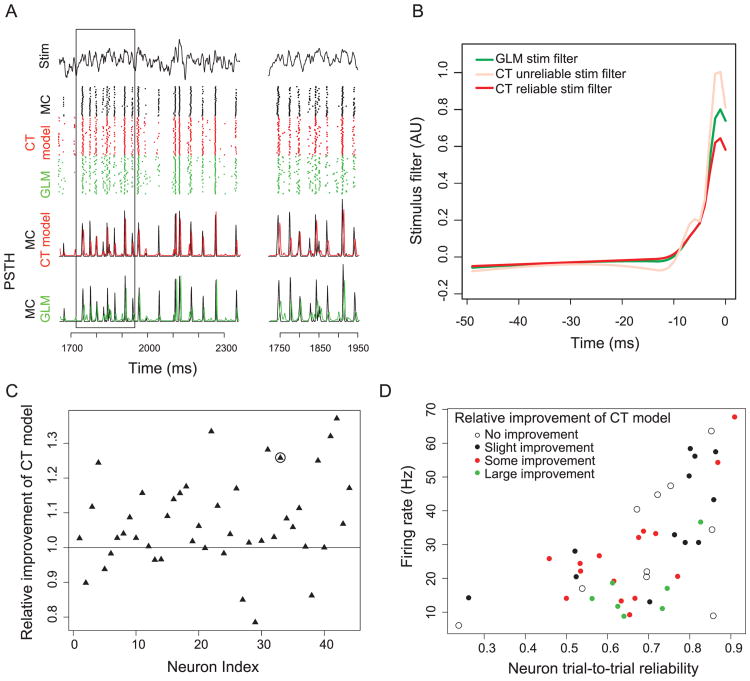
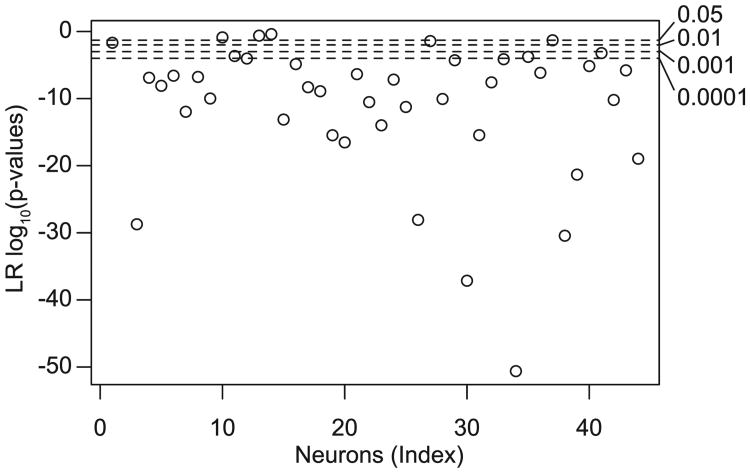
We used equations 2.1 and 2.2 to model the spiking activity of olfactory bulb MCs recorded in vitro (see Figure 1A; see also Figure 2). As described in Padmanabhan and Urban (2010) and Tripathy et al. (2013), MCs were stimulated using somatic current injection of repeated trials of frozen noise plus a DC bias while fast synaptic activity was blocked pharmacologically (n = 44 MCs, approximately 40 trials per neuron). The CT model, which treats temporally reliable spikes (based on the trial-averaged PSTH) as occurring due to a different stimulus waveform than temporally unreliable spikes (see Figure 1B), was better able to account for dynamic MC activity than the standard GLM model. We found this to be especially true for neurons with epochs of highly precise spiking (see Figure 1A, inset). Specifically, based on the PSTH error for reliable spikes (quantified as the sum of squared errors in the spike timing of reliable PSTH peaks; see the appendix), we found that on average, the CT model reduces the PSTH error relative to the GLM model by 7.5%, but in some neurons, the error reduction was as high as 37% of PSTH error (see Figure 1C). Applying a likelihood ratio test to both the GLM and CT model, we found that the CT model was significantly improved for nearly all neurons, as shown in Figure 3. (P-values for 40 of 44 were less than .05, and most were much smaller; 8 degrees of freedom difference between the two models.)
Figure 1.
Comparison of generalized linear model (GLM) and current thresholded model (CT model) in capturing dynamic mitral cell (MC) spiking activity. (A) MC intrinsic properties are probed using filtered broadband frozen noise (first row) injected into the soma. MC spike rasters (second row; black) and PSTH (third row; black) for repeated stimulus presentations (n = 40 trials). Corresponding model-based rasters and PSTHs for GLM (green) and CT model (red) show that the CT model better captures temporally precise MC spiking activity. PSTH smoothed with gaussian with σ = 2 ms and are slightly offset for visual clarity. The inset on the right indicates boxed segment on left. Data shown here include only test data not used to train model parameters. (B) Model stimulus filters for GLM (green) and CT model (unreliable stimulus filter, light red; reliable stimulus filter, dark red) for a representative MC. t = 0 ms indicates current time bin. (C) Relative improvement of CT model (with a = 1) compared to GLM. Improvement is quantified by first calculating the sum of squared errors between MC and model PSTHs and then calculating the ratio between GLM and CT model SSE. Higher ratios indicate that the CT model is a better model for MC activity than GLM. The x-axis indicates MC identity (n = 44 MCs). The circle indicates MC shown in panel A. (D) Analysis of MC features compared to CT model improvement relative to GLM. The x-axis indicates neuron trial-to-trial reliability, computed as the proportion of PSTH peaks defined as reliable relative to all PSTH peaks. The MCs split into four categories based on CT model improvement (with a = 1) relative to standard GLM model: no improvement (white; ratio of SSE < 1.0), slight improvement (black; 1.0 ≤ ratio of SSE < 1.05), some improvement (red; 1.05 ≤ ratio of SSE < 1.2), and large improvement (green; ratio of SSE ≥ 1.2).
Figure 2.
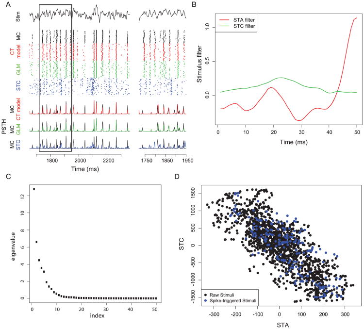
Comparison of the spike-triggered covariance model to the CT model and GLM for the example neuron highlighted in Figure 1A. (A) Rasters and PSTHs comparing each model to MC spike trains. Note that STC rasters are a much poorer model for MC activity relative to either the GLM and CT model. (B) Stimulus filters for the STC model. The STC filter corresponds to the filter with the largest eigenvalue. (C) Eigenvalues for STC eigenvectors. A single STC eigenvector with the largest eigenvalue was chosen for the STC model, in addition to the STA. (D) Density plot for stimulus snippet projection onto STA and STC bases for all stimuli (raw stimuli) and only those preceding spikes (spike-triggered stimuli). This 2D density plot was used for calculating the firing rate nonlinearity.
Figure 3.
Log-likelihood ratio p-values for testing CT versus GLM model, on a scale of log10(p), for N = 44 mitral cells.
Furthermore, by allowing the parameter a in equation 2.2 to vary, an additional 16% reduction of the PSTH error was obtained for the CT model on average (e.g., an additional 33% reduction of the PSTH error was found for the neuron in Figure 1A, for a = 1.4). While introducing the parameter a to the GLM also facilitates further model improvement (e.g., 23% improvement for the neuron in Figure 1A), the CT model still outperformed the GLM model.
Moreover, a nonlinear model incorporating an explicit additional interaction term between the stimulus and spike history filter (in lieu of the two-filter CT model) showed no improvement over the standard GLM (mean improvement = −11%), suggesting that temporally reliable spikes do not occur due to the interaction of stimulus and spike-history-based effects (e.g., stimulus-specific bursting effects). Note that both the GLM and CT model contain a linear postspike history term, which we previously found to be essential in capturing membrane resonance-like properties of MCs (Tripathy et al., 2013). For example, a spike-triggered covariance model is similar to the CT model in that both incorporate two stimulus filters (Schwartz, Pillow, Rust, & Simoncelli, 2006), but the STC model does not have a post-spike history term. We found the STC model to be qualitatively less effective for modeling the MC in Figure 1A than either the GLM or CT model (see Figure 6 in the appendix), again highlighting the importance of capturing spike history effects for these neurons.
Figure 6.
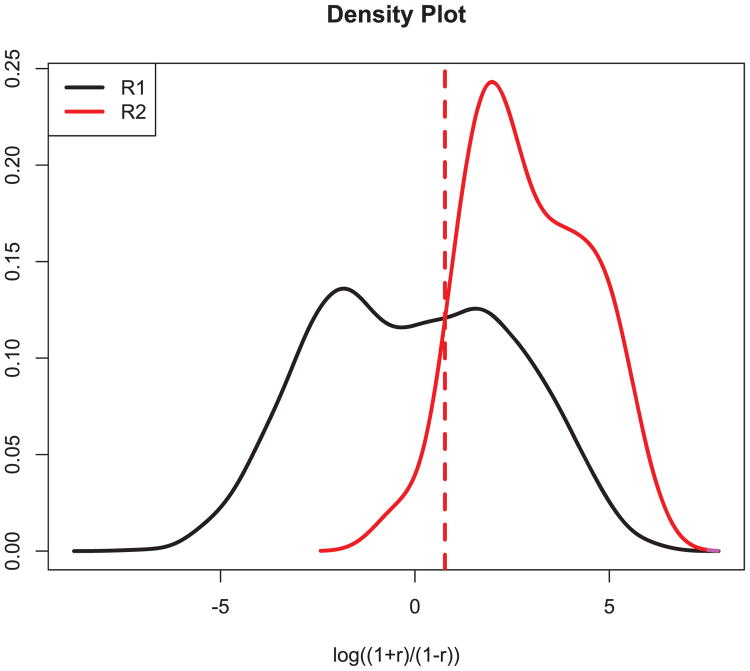
Finding the threshold using distributions of R1 and R2. In this figure, the solid black line is the fitted pdf of log((1 + R1)/(1 − R1)), and the solid purple line is the corresponding fitted pdf of log((1 + R2)/(1 − R2)). The threshold can be taken at the intersection of the two fitted pdfs.
We found that specific MCs were considerably better modeled using the CT model over the GLM. Investigating these neurons, we found that the neurons most improved were those with relatively low firing rates (10 to 35 Hz) and intermediate values of trial-to-trial reliability (see Figure 1D). In other words, the CT model was most influential for neurons that displayed a number of both reliable spikes as well as unreliable spikes. One biological explanation for this finding of differential explanatory benefits of the CT model may the inherent biophysical heterogeneity among MCs (Padmanabhan & Urban, 2010, 2014; Angelo & Margrie, 2011; Angelo et al., 2012; Burton & Urban, 2014).
4 Discussion
The empirical approach we developed here is different in spirit and detail from biophysical modeling based on intrinsic membrane responses (Hodgkin & Huxley, 1952). Whereas Hodgkin-Huxley models are useful and attractive for their direct comparison to neuronal membranes and ion channels, point processes provide the natural probabilistic framework for analyzing noisy neural spiking behavior.
An interesting shortcoming of the standard stimulus-response GLM in equation 2.1 is its failure to adequately account for spike timing reliability. We have shown that the nonlinear CT model in equation 2.2 can improve on the standard GLM, specifically, when applied to spike trains elicited in vitro during dynamic current injection. The CT model is conceptually similar to linear models, which incorporate multiple stimulus filters, such as spike-triggered covariance methods (STC) (Schwartz et al., 2006). However, the CT model differs in that it dynamically switches between one of two stimulus filters and, critically, allows for a spike history term that captures refractory and burst firing, which governs much of the precise spiking timing of mitral cells. Thus our approach extends earlier efforts to mitigate the influence of spike history effects by separately analyzing spikes well isolated in time from preceding spikes using a multi-filter approach (Agüera y Arcas & Fairhall, 2003; Agüera y Arcas, Fairhall, & Bialek, 2003).
However, we do not intend to propose this model as either realistic or empirically definitive. In the first place, additional nonlinearities are clearly needed to capture more of the spike reliability. Second, the CT model does not appear to be obviously close to any biophysical or dynamical model. Moreover, the specific methodology for fitting the CT model is admittedly somewhat ad hoc, and it may be possible to define an alternative model using parameters that can be fitted in a unified procedure.
An alternative to setting a hard threshold for reliable spiking would be to take a conceptually similar approach to that in (Escola, Fontanini, Katz, & Paninski, 2011) and use a hidden Markov model to determine whether each epoch of MC spiking activity most corresponded to that of two states: a reliable state or an unreliable state. However, since we were injecting current directly into each MC's soma, it seemed more natural to classify the neuron's effective state using the stimulus waveform directly.
While our focus here was to better model reliable MC spiking elicited during somatic current injection, our approach could likely also be extended to capture reliable spiking occurring during stimulation via naturalistic sensory stimuli such as visual scenes or auditory stimuli (Butts et al., 2007; Calabrese et al., 2011). However, we expect that as the dimensionality of the stimulus increases, more data will be required to adequately parameterize each of the two stimulus filters used here. Our two-filter approach could also be applied in conjunction with other approaches for modeling reliable spiking, such as those that explicitly model the effects of threshold nonlinearities of afferent presynaptic neurons (Butts, Weng, Jin, Alonso, & Paninski, 2011).
Given these caveats, our intention with the CT model is to use it to stimulate additional research. Perhaps a point process regression model, based on GLM methodology but again incorporating nonlinearity, might be based on ideas such as the adaptive timescale rate version of the exponential LIF model of Ostojic and Brunel (2011). By working at the interface between statistical and dynamical system modeling, it may be possible to gain further insight into reliable spiking.
Acknowledgments
We thank G. LaRocca for technical support. This work was supported by an NSF Graduate Research Fellowship and an R. K. Mellon Foundation Fellowship (to S.J.T.), a Crick-Jacobs Junior Fellowship and NIMH K99 MH101634 (to K.P.), NIDCD grant R01 DC011184 (to N.N.U.), and NIMH R01 MH064537 (to R.E.K). This research was funded in part by a grant from the Pennsylvania Department of Health's Commonwealth Universal Research Enhancement Program.
Appendix: Data Collection, Algorithm, and More Results
A.1 Experimental Methods and Data Collection
Whole cell patch clamp recordings of mitral cells were obtained in vitro from mouse olfactory bulb slices using methods described previously (Padmanabhan & Urban, 2010). Mitral cells were identified under infrared differential interference contrast optics on the basis of their laminar position in the olfactory bulb and their morphology. All experiments were performed at 35° C in standard Ringer's solution with excitatory (25 μM AP5 and 10 μM CNQX) and inhibitory (10 μM bicuculline) synaptic activity blocked.
Current-clamp recordings were performed while injecting neurons with a filtered white noise current stimulus. Noise traces were generated by convolving a 2.5 s white noise current with an alpha function of the form t * exp(−t/τ), where τ = 3 ms. We chose this spectral structure because it generates reliable spiking in these neurons and corresponds to the timescale of fast synapses afferent to MCs (Galán, Ermentrout, & Urban, 2008). Each neuron received one of a small number of stimuli generated using this method (most neurons received one of three stimulus templates) and was presented about 40 stimulus repeats. The amplitude (variance) of the noise used was between 5% and 40% of the direct current (100–800 pA, σ = 20–80 pA) offset for each cell, with the majority of cells receiving 10% to 20% of the DC offset. The variance of the noise was selected as previously described (Galán et al., 2008), to induce reliable firing without large input fluctuations. For all recordings, a 25 or 50 pA hyperpolarizing pulse was injected before stimuli were delivered to measure input resistance and membrane time constant, allowing us to track the stability of recordings over multiple trials. As described in Tripathy et al. (2013) only neurons whose firing patterns were stable across trials and fired a sufficient number of spikes in each trial (more than 5 Hz) were used in this study. Upon stimulation, most neurons usually underwent a brief nonspiking adaptation period (111 +/−14 ms) which was assessed visually and excluded from the analysis.
A.2 Fitting Procedure
For each neuron, our procedure may be summarized as follows:
Use the PSTH to identify reliable and unreliable peaks in the PSTH.
Define a reliable-spike current template as the longest positive part to the end of the trimmed mean of the 20 ms snippets of current preceding the reliable peaks, which is l ms.
Consider all l ms snippets of current and separate these into two categories: (1) those immediately preceding the reliable peaks and (2) all others. Find the correlation of each snippet with the reliable-spike current template and take its Fisher z transformation. This produces two distributions of values—one for category 1 and one for category 2. Then use a Bayes classifier to determine a threshold for classifying each current snippet as either a reliable-spike current or an unreliable-spike current. Also, take the snippets that have high correlation but small inner-product with current template as unreliable.
The PSTH was examined in step 1. First, we thresholded the PSTH and considered only time points within the PSTH that contained a spike in at least three trials (from among approximately 40 trials total). For convenience, we define such PSTH time points as PSTH peaks. Second, for all the PSTH peaks, we combined the neighboring peaks with time difference less than 5 ms. This step is to make sure there is no temporal separation of one PSTH big peak into multiple smaller peaks. Finally, for each PSTH peak, we recorded the temporal range of the peak and calculated the percentage of trials that spike in that range. If the percentage was bigger than 90% (e.g., 36 of 40 trials) and the temporal range was smaller than 12 ms, we regarded that peak as reliable. Otherwise we called it unreliable. When we report neuron reliability, it is defined as the proportion of reliable peaks among all the peaks for the neuron.
Considering the set of 20 ms current snippets immediately preceding these reliable PSTH peaks, in step 2, we computed the mean 20 ms snippet (the mean across all these peaks). Because a positive current is required to drive each neuron to spike, we take only the positive portion of this snippet. We next computed the correlation of each snippet with the mean and excluded as outliers any snippets that have correlation greater than 1.5 times standard deviations from the mean correlation. We then recomputed the mean snippet to get the reliable-spike current template.
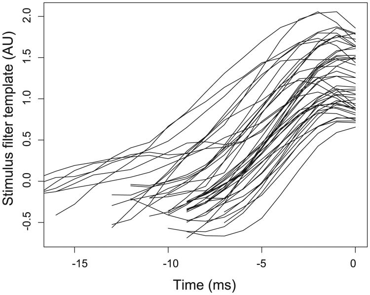
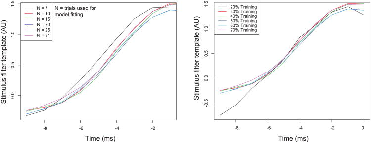
In Figure 4 we display the reliable-spike current templates computed for each of the mitral cells. In Figure 5 we show how the reliable-spike current template varies as a function of trials and peristimulus time used for model fitting. It may be seen that the parameter fits for the reliable spike template stabilized with a relatively small number of trials (n > 10 trials). Similarly, for n > 10 trials, more than 90% of the reliable PSTH peaks are recovered relative to when all trials are used to identify the reliable PSTH peaks. With respect to stimulus time, the reliable spike template converges when at least 30% of the total stimulus is used for training data relative to the 70% used previously (.75 s vs 1.75 s).
Figure 4.
Reliable stimulus current templates shown for all of the mitral cells. N = 44 mitral cells.
Figure 5.
Convergence of reliable current stimulus template as a function of the number of trials used to fit the model (left) or amount of training data with respect to time for model fitting (right). Stimulus filter template shown for the neuron highlighted in Figure 1A. In both cases, a relatively small amount of training data, both with respect to trials or peristimulus time, is needed for stimulus filter template to empirically converge.
In step 3, we computed the correlation of each snippet with the reliablespike current template, applied the Fisher z transformation , and thereby obtained z-transformed correlations for the snippets within each of two categories: (1) those immediately preceding the reliable peaks (termed R2) and (2) all others (termed R1). We then applied a Bayes classifier (Kass et al., 2014; Hastie, Tibshirani, & Friedman, 2011) to find the threshold, as the intersection of the density functions for the correlations under both cases, that best discriminated these transformed coefficients (see Figure 6).
Also, we computed the inner product of each snippet with reliable current template, and take the snippets with inner product larger than mean (Inner-products) – sd (Inner-products). This ensures that classified reliable current snippets are those that have high correlation with the reliable current template and those that have large absolute current magnitude that could inspire a spike.
After these steps, we finally have the classification of stimulus and can define our two stimulus kernel k1 and k2 in the model. If time t was regarded as a reliable-spike time, we used the convolution of k1 and 50 ms before t in the stimulus term; if unreliable, we used the convolution of k2 and 50 ms before t in the stimulus term. Model fitting proceeded by maximizing the likelihood function, as usual. We used seven nonlinearly spaced spline knots to fit k⃗ and 6 knots to fit h⃗ (Pillow et al., 2008; Tripathy et al., 2013). In practice, we replace (k⃗rel∙x⃗i, rel)a with sign(k⃗rel ∙ x⃗i, rel)|k⃗rel x⃗i, rel|a.
A.3 Assessing Model Goodness of Fit
We used the summation of squared errors (SSE) as the goodness-of-fit measure for the models used here. Specifically, we used the difference between the PSTH for data and simulated spike trains. With the initial 70% of original data (with respect to peristimulus time, but including all trials) as training data, we fit each model and found model parameters. With these fitted filters and given stimuli, we next simulated 300 spike trains for each neuron. The simulated spike trains were used as simulated data.
For each reliable peak from test data, we compared the mean spike time of this peak and the simulated PSTH. The summation of the squared difference between the mean time of both real and simulated PSTH peaks is denoted as SSE for reliable spikes.
To define the likelihood ratio test to compare the GLM and CT models, we use the first 50% of the stimulus and spike train data to train the reliable current template for the CT model and the last 50% data to fit both models.
Contributor Information
Wanjie Wang, Department of Statistics, Carnegie Mellon University, Pittsburgh, PA 15213, U.S.A.
Shreejoy J. Tripathy, Center for the Neural Basis of Cognition, Carnegie Mellon University, Pittsburgh, PA 15213, U.S.A
Krishnan Padmanabhan, Department of Biology, Carnegie Mellon University, Pittsburgh, PA 15213, U.S.A.
Nathaniel N. Urban, Center for the Neural Basis of Cognition and Department of Biology, Carnegie, Mellon University, Pittsburgh, PA 15213, U.S.A
Robert E. Kass, Department of Statistics, Machine Learning Department, and Center for the Neural Basis of Cognition, Carnegie Mellon University, Pittsburgh, PA 15213, U.S.A
References
- Agüera y Arcas B, Fairhall AL. What causes a neuron to spike? Neural Computation. 2003;15(8):1789–1807. doi: 10.1162/08997660360675044. [DOI] [PubMed] [Google Scholar]
- Agüera y Arcas B, Fairhall AL, Bialek W. Computation in a single neuron: Hodgkin and Huxley revisited. Neural Computation. 2003;15(8):1715–1749. doi: 10.1162/08997660360675017. [DOI] [PubMed] [Google Scholar]
- Angelo K, Margrie TW. Population diversity and function of hyperpolarization-activated current in olfactory bulb mitral cells. Scientific Reports. 2011;1 doi: 10.1038/srep00050. [DOI] [PMC free article] [PubMed] [Google Scholar]
- Angelo K, Rancz EA, Pimentel D, Hundahl C, Hannibal J, Fleischmann A, et al. Margrie TW. A biophysical signature of network affiliation and sensory processing in mitral cells. Nature. 2012;488(7411):375–378. doi: 10.1038/nature11291. [DOI] [PMC free article] [PubMed] [Google Scholar]
- Badel L, Lefort S, Berger T, Petersen C, Gerstner W, Richardson M. Extracting non-linear integrate-and-fire models from experimental data using dynamic I–V curves. Biological Cybernetics. 2008;99(4):361–370. doi: 10.1007/s00422-008-0259-4. [DOI] [PMC free article] [PubMed] [Google Scholar]
- Bryant HL, Segundo JP. Spike initiation by transmembrane current: A white-noise analysis. Journal of Physiology. 1976;260(2):279–314. doi: 10.1113/jphysiol.1976.sp011516. [DOI] [PMC free article] [PubMed] [Google Scholar]
- Burton SD, Urban NN. Greater excitability and firing irregularity of tufted cells underlies distinct afferent-evoked activity of olfactory bulb mitral and tufted cells. Journal of Physiology. 2014;592(10):2097–2118. doi: 10.1113/jphysiol.2013.269886. [DOI] [PMC free article] [PubMed] [Google Scholar]
- Butts DA, Weng C, Jin J, Alonso JM, Paninski L. Temporal precision in the visual pathway through the interplay of excitation and stimulus-driven suppression. Journal of Neuroscience. 2011;31(31):11313–11327. doi: 10.1523/JNEUROSCI.0434-11.2011. [DOI] [PMC free article] [PubMed] [Google Scholar]
- Butts DA, Weng C, Jin J, Yeh CI, Lesica NA, Alonso JM, Stanley GB. Temporal precision in the neural code and the timescales of natural vision. Nature. 2007;449(7158):92–95. doi: 10.1038/nature06105. [DOI] [PubMed] [Google Scholar]
- Calabrese A, Schumacher JW, Schneider DM, Paninski L, Woolley SMN. A generalized linear model for estimating spectrotemporal receptive fields from responses to natural sounds. PLoS ONE. 2011;6(1):e16104. doi: 10.1371/journal.pone.0016104. [DOI] [PMC free article] [PubMed] [Google Scholar]
- Doya K. Bayesian brain: Probabilistic approaches to neural coding. Cambridge, MA: MIT Press; 2011. [Google Scholar]
- Escola S, Fontanini A, Katz D, Paninski L. Hidden Markov models for the stimulus-response relationships of multistate neural systems. Neural Computation. 2011;23(5):1071–1132. doi: 10.1162/NECO_a_00118. [DOI] [PubMed] [Google Scholar]
- Galán RF, Ermentrout GB, Urban NN. Optimal time scale for spike-time reliability: Theory, simulations, and experiments. Journal of Neurophysiology. 2008;99(1):277–283. doi: 10.1152/jn.00563.2007. [DOI] [PMC free article] [PubMed] [Google Scholar]
- Giridhar S, Doiron B, Urban NN. Timescale-dependent shaping of correlation by olfactory bulb lateral inhibition. Proceedings of the National Academy of Sciences. 2011;108:5843–5848. doi: 10.1073/pnas.1015165108. [DOI] [PMC free article] [PubMed] [Google Scholar]
- Hastie T, Tibshirani R, Friedman J. The elements of statistical learning: Data mining, inference, and prediction (2nd ed) New York: Springer; 2011. [Google Scholar]
- Hodgkin AL, Huxley AF. A quantitative description of membrane current and its application to conduction and excitation in nerve. Journal of Physiology. 1952;117(4):500–544. doi: 10.1113/jphysiol.1952.sp004764. [DOI] [PMC free article] [PubMed] [Google Scholar]
- Izhikevich EM. Dynamical systems in neuroscience: The geometry of excitability and bursting. Cambridge, MA: MIT Press; 2010. [Google Scholar]
- Kass RE, Eden U, Brown EN. Analysis of neural data. New York: Springer; 2014. [Google Scholar]
- Kass RE, Ventura V. A spike-train probability model. Neural Computation. 2001;13(8):1713–1720. doi: 10.1162/08997660152469314. [DOI] [PubMed] [Google Scholar]
- Kelly RC, Smith MA, Kass RE, Lee TS. Local field potentials indicate network state and account for neuronal response variability. Journal of Computational Neuroscience. 2010;29:567–579. doi: 10.1007/s10827-009-0208-9. [DOI] [PMC free article] [PubMed] [Google Scholar]
- Koch C. Biophysics of computation: Information processing in single neurons. New York: Oxford University Press; 1999. [Google Scholar]
- Mainen ZF, Sejnowski TJ. Reliability of spike timing in neocortical neurons. Science. 1995;268(5216):1503–1506. doi: 10.1126/science.7770778. [DOI] [PubMed] [Google Scholar]
- Mensi S, Naud R, Pozzorini C, Avermann M, Petersen CCH, Gerstner W. Parameter extraction and classification of three cortical neuron types reveals two distinct adaptation mechanisms. Journal of Neurophysiology. 2012;107(6):1756–1775. doi: 10.1152/jn.00408.2011. [DOI] [PubMed] [Google Scholar]
- Ostojic S, Brunel N. From spiking neuron models to linear-nonlinear models. PLoS Computational Biology. 2011;7(1):e1001056. doi: 10.1371/journal.pcbi.1001056. [DOI] [PMC free article] [PubMed] [Google Scholar]
- Padmanabhan K, Urban NN. Intrinsic biophysical diversity decorrelates neuronal firing while increasing information content. Nature Neuroscience. 2010;13(10):1276–1282. doi: 10.1038/nn.2630. [DOI] [PMC free article] [PubMed] [Google Scholar]
- Padmanabhan K, Urban NN. Disrupting information coding via block of 4-AP sensitive potassium channels. Journal of Neurophysiology. 2014;12:1054–1066. doi: 10.1152/jn.00823.2013. [DOI] [PMC free article] [PubMed] [Google Scholar]
- Paninski L. Maximum likelihood estimation of cascade point-process neural encoding models. Network. 2004;15(4):243–262. [PubMed] [Google Scholar]
- Paninski L, Pillow JW, Simoncelli EP. Maximum likelihood estimation of a stochastic integrate-and-fire neural encoding model. Neural Computation. 2004;16(12):2533–2561. doi: 10.1162/0899766042321797. [DOI] [PubMed] [Google Scholar]
- Pillow JW, Shlens J, Paninski L, Sher A, Litke AM, Chichilnisky EJ, Simoncelli EP. Spatio-temporal correlations and visual signalling in a complete neuronal population. Nature. 2008;454(7207):995–999. doi: 10.1038/nature07140. [DOI] [PMC free article] [PubMed] [Google Scholar]
- Schwartz O, Pillow JW, Rust NC, Simoncelli EP. Spike-triggered neural characterization. Journal of Vision. 2006;6(4):484–507. doi: 10.1167/6.4.13. [DOI] [PubMed] [Google Scholar]
- Tiesinga P, Fellous JM, Sejnowski TJ. Regulation of spike timing in visual cortical circuits. Nature Reviews Neuroscience. 2008;9(2):97–107. doi: 10.1038/nrn2315. [DOI] [PMC free article] [PubMed] [Google Scholar]
- Tripathy SJ, Padmanabhan K, Gerkin RC, Urban NN. Intermediate intrinsic diversity enhances neural population coding. Proceedings of the National Academy of Sciences. 2013;110(20):8248–8253. doi: 10.1073/pnas.1221214110. [DOI] [PMC free article] [PubMed] [Google Scholar]


