A detailed comparison of optimality and simplicity in perceptual decision-making

Abstract

Two prominent ideas in the study of decision-making have been that organisms behave near-optimally, and that they use simple heuristic rules. These principles might be operating in different types of tasks, but this possibility cannot be fully investigated without a direct, rigorous comparison within a single task. Such a comparison was lacking in most previous studies, because a) the optimal decision rule was simple; b) no simple suboptimal rules were considered; c) it was unclear what was optimal, or d) a simple rule could closely approximate the optimal rule. Here, we used a perceptual decision-making task in which the optimal decision rule is well-defined and complex, and makes qualitatively distinct predictions from many simple suboptimal rules. We find that all simple rules tested fail to describe human behavior, that the optimal rule accounts well for the data, and that several complex suboptimal rules are indistinguishable from the optimal one. Moreover, we found evidence that the optimal model is close to the true model: first, the better the trial-to-trial predictions of a suboptimal model agree with those of the optimal model, the better that suboptimal model fits; second, our estimate of the Kullback-Leibler divergence between the optimal model and the true model is not significantly different from zero. When observers receive no feedback, the optimal model still describes behavior best, suggesting that sensory uncertainty is implicitly represented and taken into account. Beyond the task and models studied here, our results have implications for best practices of model comparison.

Many forms of human perception seem close to the ideal set by Bayesian optimality (Geisler, 2011; Körding et al., 2007), according to which the brain maximizes performance given noisy and ambiguous sensory input. In most of these cases, such as in cue combination (e.g. Alais & Burr, 2004; Ernst & Banks, 2002; Gu, Angelaki, & Deangelis, 2008; for more examples, see Trommershauser, Körding, & Landy, 2011), the optimal decision rule is simple. It has been argued that when the optimal decision rule is complex, the brain has an incentive to use a computationally simple and reasonably effective, though strictly suboptimal decision rule – also called a heuristic (Gigerenzer & Gaissmaier, 2011; Simon, 1956).

Evidence for this proposal has been mixed. On the one hand, there is no strong evidence for optimality in complex tasks. In some studies that claim that people follow a complex optimal rule, simple suboptimal rules were not considered (e.g. Geisler & Perry, 2009; see also Bowers and Davis, 2012). In other studies, the optimal rule fitted about equally well as a simple rule (Mazyar, Van den Berg, & Seilheimer, 2013; Palmer, Verghese, & Pavel, 2000; Qamar et al., 2013). In some perceptual experiments, the optimal rule outperformed simple rules, but only a few simple rules were tested (Ma, Navalpakkam, Beck, van Den Berg, & Pouget, 2011; Ma, Shen, Dziugaite, & van den Berg, 2015). Finally, it has been argued that in reports of near-optimality in cognitive tasks (Chater, Tenenbaum, & Yuille, 2006; Norris, 2006), the optimal model was given excessive flexibility in order to fit the data (Bowers & Davis, 2012; Gigerenzer, 2004; Jones & Love, 2011), making the optimality label suspect.

On the other hand, some claims of suboptimality might be premature. For ball-catching, a suboptimal but simple “gaze heuristic” has been proposed (Dienes & McLeod, 1996; McLeod, Reed, & Dienes, 2003). However, in such complex sensorimotor tasks, the definition of optimality depends on largely unknown costs, making it difficult to conclusively claim that behavior is suboptimal; in fact, in a simplified setting, ball-catching was found to be near-optimal (Faisal & Wolpert, 2009; López-Moliner, Field, & Wann, 2007).

Thus, optimality and simplicity have so far not been directly compared in a strongly distinguishing paradigm. In addition, none of the above studies made an effort to establish how much room there is for an untested model to fit better than the study’s favored model, whether optimal or simple. To address both issues, we used a visual categorization task that did not suffer from the shortcomings above: optimality was not ambiguous, and there are many plausible simple rules that make substantially different predictions from the optimal rule. Moreover, in analyzing the data from this task, we attempt to establish how close our best-fitting model is to the unknown true model.

We want to emphasize that in this paper, ‘simplicity’ refers to the number of operations in the observer’s decision rule. In previous literature, simplicity has been used in at least two other meanings. The first is the simplicity of the observer’s interpretation of a visual scene. The “simplicity principle”, initiated by Wertheimer and other Gestalt psychologists, states that the observer reports the simplest interpretation of a visual scene that is consistent with the sensory input, for example leading to a preference for perceiving continuity (Chater, 1996). In our task, the two hypotheses about the state of the world, left and right, are equally complex in this sense. The second meaning is simplicity in terms of the number of parameters (Spiegelhalter, Best, Carlin, & Van Der Linde, 2002). In our case, all the models we will discuss below have two parameters, and the only thing that differs is the observer’s decision rule. Thus, we are not talking about simplicity from the point of view of the experimenter comparing models, but about simplicity from the point of view of the observer doing the task.

EXPERIMENT 1

We designed our experiment such that the statistical structure of the task was easy for subjects to learn, but optimal inference was hard. The task was a visual target categorization task on four oriented stimuli. On each trial, we presented observers with a target and three identical distractors (Fig. 1A); the target orientation and the (common) distractor orientation were drawn independently from the same Gaussian distribution with a mean of vertical and a standard deviation of σ_s=9.06° (Fig. 1B). Subjects reported whether the target stimulus was tilted to the right or to the left of vertical. Correctness feedback was provided on each trial.

Figure 1. Task and data.

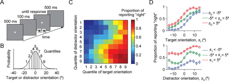
(A) Trial procedure. Each display contains four items, three of which have a common orientation; these are the distractors. Subjects report whether the fourth item (the target) is tilted to the left or to the right with respect to vertical. The target location is randomly chosen on every trial. (B) The target orientation and the common distractor orientation are independently drawn from the same Gaussian distribution with a mean of 0° (vertical) and a standard deviation of 9.06°. For plotting purposes, we divided orientation space into 9 quantiles. (C) Proportion of reporting “right” (color) as a function of target and distractor orientation quantiles. (D) Proportion of reporting “right” as a function of target orientation s_T (top) and distractor orientation s_D (top). Error bars are s.e.m. The top curves are not expected to be monotonic (see text).

Apparatus and stimuli

Subjects were seated at a viewing distance of approximately 60 cm. All stimuli were displayed on a 21-inch LCD monitor with a refresh rate of 60 Hz and a resolution of 1280 by 1024 pixels. The background luminance was approximately 29.3 cd/m². Each stimulus display contained four stimuli, placed on an invisible circle centered at the center of the screen and with a radius of 5° of visual angle. The angular positions of the stimuli were −135°, −45°, 45°, and 135° relative to the positive horizontal axis. Each stimulus was a Gabor patch with a peak luminance of approximately 35.2 cd/m², a spatial frequency of 3.13 cycles per degree, a standard deviation of 8.18 pixels, and a phase of 0. On each trial, three of the stimuli were identical; these were distractors. The fourth stimulus, whose location was chosen from the four possible locations with equal probabilities, was the target. Target and distractor orientations were independently drawn from a Gaussian distribution with a mean of 0° (vertical) and a standard deviation of 9.06°.

Experimental procedure

Each trial started with a fixation dot on a blank screen (500 ms), followed by a stimulus display (50 ms). Then a blank screen was shown until the subject made a response. Subjects pressed a button to report whether the target was tilted to the right or to the left relative to vertical. After the response, correctness feedback was given by coloring the fixation dot red or green (500 ms) (Fig. 1A).

The experiment consisted of three sessions on different days. Each session consisted of 5 blocks, and each block contained 200 trials, for a total of 3 × 5 × 200 = 3000 trials per subject. To avoid the learning effect, data from the first session (1000 trials) were excluded in the analysis. Nine subjects participated in this study (seven female, age range 23 to 30 years), all of them scientifically trained but naïve to the task. At the beginning of the first session, subjects were orally briefed about all detailed experimental designs including the descriptions about the stimulus distribution: the target orientation and the common distractor orientation are drawn from the same bell-shaped distribution; the orientations occur most often at vertical and the width of the distribution is 9.06° (Fig. 1B).

Experiment 1 data

Human behavior in this task exhibits several interesting patterns (Fig. 1C). The proportion of “right” responses increases monotonically with target orientation (Fig. 1D, top), but also depends on distractor orientation. More surprising is that the proportion of “right” responses does not increase monotonically with distractor orientation (Fig. 1D, bottom). On second thought, this is intuitive: suppose the target is vertical, and the distractors are slightly tilted to the right. Then, the distractors can easily be confused with the target, and therefore the subject will often report “right”. By contrast, when the distractors are strongly tilted to the right, they are easily identified as distractors and a sophisticated subject will only use the item that is most likely to be the target in their response (in this example, make a random guess).

MODELS

We study four categories of models: the optimal model, simple heuristic models, two-step models, and generalized sum models.

The optimal model

The optimal observer has learned the generative model of the task and incorporates this knowledge during decision-making. We first discuss the generative model (Fig. 2A). We denote the binary variable C the direction of tilt relative to vertical (−1 for left, +1 for right). A distractor orientation s_D is drawn from a Gaussian distribution with a mean of 0 and a standard deviation of σ_s. A target orientation s_T is drawn from that same Gaussian distribution but truncated to only negative values (when C=−1) or only positive values (when C=1); thus, the conditional distribution of s_T is a half-Gaussian. Stimuli appear at four fixed locations. The target location, L, is chosen with equal probability for each of the four possibilities. The orientation at that location is s_T, and the orientations at the three other locations are all s_D. Finally, we assume that the observer makes a noisy measurement x_i of each orientation. We assume that each x_i is independently drawn from a Gaussian distribution whose mean is the true stimulus (s_T or s_D) and whose standard deviation is σ.

Figure 2. Generative model.

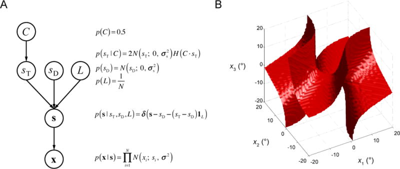
(A) Each node represents a random variable, each arrow a conditional probability distribution. Distributions are shown in the equations on the side. N(x; 0, σ²) denotes a normal distribution with a mean of 0 and a variance of σ². H(x) denotes the Heaviside function. 1_L denotes a vector in which the L^th entry equals 1 and all others equal 0. δ(x) is the Dirac delta function. This diagram specifies the distribution of the measurements, x. The optimal observer inverts the generative model and computes the conditional probability of C given x. (B) Decision boundary of the optimal decision rule if the set size N were equal to 3. Each point in the three-dimensional space represents a set of measurements x = (x₁, x₂, x₃). On one side of the boundary (the side that includes the all-positive octant), the optimal observer reports “right”, on the other side, “left”.

We are now ready to describe the optimal observer’s inference process. Given a set of measurements x = (x₁, x₂, x₃, x₄), the optimal observer considers each item a potential target and computes the weighted average over locations L of the probability that an assumed target at L was tilted right, with weight given by the probability that the target was at L. The posterior over C (C=1 or −1) is

$$p\left(C|\mathbf{x}\right)={\displaystyle \sum _{L=1}^{N}p\left(C|\mathbf{x},L\right)p\left(L|\mathbf{x}\right),}$$ (1)

where N denotes the set size (in our case, N=4). Eq. (1) represents a weighted average over L, which is an example of the Bayesian operation of marginalization. We can simplify Eq. (1) to

$$\begin{array}{l}p\left(C|\mathbf{x}\right)={\displaystyle \sum _{L=1}^N\frac{p\left(\mathbf{x}|C,L\right)}{\left(\mathbf{x}|L\right)}p\left(C\right)p\left(\mathbf{x}|L\right)\frac{p\left(L\right)}{p\left(\mathbf{x}\right)}}\\ =\frac{p\left(\mathbf{C}\right)}{p\left(\mathbf{x}\right)}{\displaystyle \sum _{L=1}^{N}p\left(\mathbf{x}|C,L\right)p\left(\mathbf{x}|L\right).}\end{array}$$ (2)

Given that the priors over C and L are uniform, and p(x) is just a normalization, we only need to compute p(x|C,L), the likelihoods of C=±1 given L. To compute these, the optimal observer marginalizes over all unknown variables other than C and L. These variables are the stimulus orientations s, the values of target and distractor orientations, s_T and s_D.

$$\begin{array}{l}p\left(\mathbf{x}|C,L\right)=\int p\left(\mathbf{x}|\mathbf{s}\right)p\left(\mathbf{s}|C,L\right)d\mathbf{s}\\ =\iiint p\left(\mathbf{x}|\mathbf{s}\right)p\left(\mathbf{s}|s_{\mathrm{T}},s_{\mathrm{D}},L\right)p\left(s_{\mathrm{T}},s_{\mathrm{D}}|C\right)d\mathbf{s}d{s}_{\mathrm{T}}d{s}_{\mathrm{D}}\\ ={\displaystyle \iiint \left({\displaystyle \prod _{i=1}^{N}p\left(x_i|s_i\right)}\right)}\delta \left(\mathbf{s}-s_{\mathrm{D}}-\left(s_{\mathrm{T}}-s_{\mathrm{D}}\right){\mathbf{1}}_L\right)p\left(s_{\mathrm{T}}|C\right)p\left(s_{\mathrm{D}}\right)d\mathbf{s}d{s}_{\mathrm{T}}d{s}_{\mathrm{D}}\\ =\left({\displaystyle \int p\left(x_L|s_{\mathrm{T}}\right)p\left(s_{\mathrm{T}}|C\right)d{s}_{\mathrm{T}}}\right)\left({\displaystyle \int \left({\displaystyle \prod _{i\ne L}p\left(x_i|s_{\mathrm{D}}\right)}\right)p\left(s_{\mathrm{D}}\right)d{s}_{\mathrm{D}}}\right),\end{array}$$ (3)

where 1_L is a vector of zeroes except for a 1 in the L^th dimension and δ(x) is Dirac delta function.

The optimal observer reports “right” when the posterior probability of a right tilt, p(C=1|x), exceeds the posterior probability of a left tilt, p(C=−1|x). Starting from Eq. (2), we see that this is the case when

$${\displaystyle \sum _{L=1}^{N}p\left(\mathbf{x}|C=1,L\right)}>{\displaystyle \sum _{L=1}^{N}p\left(\mathbf{x}|C=-1,L\right)}.$$ (4)

Evaluating Eq. (3) and then substituting in Eq. (4), we find that the optimal decision rule (Opt rule) is to report “right” when

$${\displaystyle \sum _{L=1}^N{e}^{{\text{Weight}}_L\left(\mathbf{x}\right)}}\text{erf}\frac{\frac{x_L}{{\sigma }^2}}{\sqrt{2\left(\frac{1}{{\sigma }^2}+\frac{1}{{\sigma }_{\mathrm{s}}^2}\right)}}>0,$$ (5)

where Weight_i(x) reflects the strength of the evidence that the target is at L:

$${\text{Weight}}_L\left(\mathbf{x}\right)=-\frac{x_L^2}{2\left({\sigma }_{\mathrm{s}}^2+{\sigma }^2\right)}-\frac{{\overline{\mathbf{x}}}_{\backslash L}^2}{2\left({\sigma }_{\mathrm{s}}^2+\frac{{\sigma }^2}{N-1}\right)}-\frac{N-1}{2{\sigma }^2}\mathrm{var}{\mathbf{x}}_{\backslash L}.$$ (6)

Here, ${\overline{\mathbf{x}}}_{\backslash L}$ and Var ${\mathbf{x}}_{\backslash L}$ are the sample mean and variance of x with the L^th element left out, respectively. The first term in the expression for Weight_L(x) comes from ${\displaystyle \int p\left(x_L|s_{\mathrm{T}}\right)p\left(s_{\mathrm{T}}|C\right)d{s}_{\mathrm{T}}}$ and the other two terms come from ${\displaystyle \int \left({\displaystyle \prod _{i\ne L}p\left(x_i|s_{\mathrm{D}}\right)}\right)p\left(s_{\mathrm{D}}\right)d{s}_{\mathrm{D}}}$ in Eq.(3). To aid our intuition, we visualize the optimal decision rule for the hypothetical scenario that set size N=3, in Fig. 2B.

Interestingly, each of the components of the weight term has a clear intuitive meaning: they can be interpreted as being associated with the target, the distractor mean, and the distractor variance, respectively. Since both the target orientation and the common distractor orientation are drawn from a Gaussian distribution with a mean of 0, the L^th item is more likely to be the target when the L^th measurement is closer to 0 (target term), and the mean of the measurements at the other locations is closer to 0 (distractor mean term). Moreover, the subject knows that the three distractor orientations are the same, so an item is more likely to be the target when the variance of the measurements at the other three locations is smaller (distractor variance term). In the following, we will examine whether human subjects take all these aspects of the task statistics into account.

Simple heuristic models

Several simple heuristic decision rules are plausible for this task. These rules, some of which have been widely used in previous studies, postulate how the observer integrates information across locations. According to the (signed) Max rule, the observer reports the direction of tilt of the measurement that is most tilted in either direction (Baldassi & Verghese, 2002; Eckstein, 1998; Green & Swets, 1966; Nolte & Jaarsma, 1967; Palmer et al., 2000). According to the Sum rule, the observer reports the direction of tilt of the sum of the four measurements (Baldassi & Burr, 2000; Green & Swets, 1966; Kramer, Graham, & Yager, 1985; Palmer et al., 2000). We also conceived three new simple heuristics. According to the Min rule, the observer reports the direction of tilt of the measurement that is least tilted in either direction. According to the Var rule, the observer reports the direction of tilt of the measurement which, when left out, leaves the smallest variance of the remaining three measurements. Finally, according to the Sign rule, the observer reports the common direction of tilt when all measurements are tilted in the same direction, and the least frequent direction of tilt otherwise (guessing in case of a tie). All of these rules perform above chance, but they make very different predictions from the Opt rule.

Two-step models

We then considered “two-step models”, in which the observer does not marginalize over target location but instead follows a simple strategy of first deciding which item is the target, then reporting its direction of tilt. This suboptimal decision process is similar to the “Take The Best” heuristic algorithm (Gigerenzer & Goldstein, 1996), in which decisions are based solely on the cue that best discriminates between options, and to some other two-step models in perception (Fleming, Maloney, & Daw, 2013; Jazayeri & Movshon, 2007).

Different two-step models can be constructed based on how the target is selected in the first step. One way is to transform the Opt model to a two-step model by replacing the (optimal) marginalization over L in Eq. (1) with (suboptimal) maximization: the first step is to infer the target location, $\widehat{L}$, and the second step is to infer the target tilt $\widehat{C}$ given that location:

$$\begin{array}{l}\widehat{L}=\underset{L}{\text{argmax}}p\left(L|\mathbf{x}\right),\\ \widehat{C}=\underset{C}{\text{argmax}}p\left(C|\mathbf{x},\widehat{L}\right).\end{array}$$ (7)

When we evaluate the first line of Eq.(7) and make use of the fact that p(L) is uniform, we get:

$$\begin{array}{l}\widehat{L}=\underset{L}{\text{argmax}}p\left(\mathbf{x}|L\right)\frac{p\left(L\right)}{p\left(\mathbf{x}\right)}\\ =\underset{c}{\text{argmax}}p\left(\mathbf{x}|L\right)\\ =\underset{L}{\text{argmax}}\left({\displaystyle \int \left({\displaystyle \prod _{i\ne L}p\left(x_i|s_{\mathrm{D}}\right)}\right)p\left(s_{\mathrm{D}}\right)d{s}_{\mathrm{D}}}\right).\end{array}$$ (8)

Retracing the derivation from Eq. (3) to Eq. (5) shows that finding $\widehat{L}$ amounts to maximizing Weight_L(x) in Eq. (6):

$$\widehat{L}=\underset{L}{\text{argmax}}{\text{Weight}}_L(\mathbf{x}).$$ (9)

The second step is inferring the target tilt if we assume that the target location is $\widehat{L}$:

$$\begin{array}{l}\widehat{C}=\underset{C}{\text{argmax}}\frac{p\left(\mathbf{x}|C,\widehat{L}\right)}{p\left(\mathbf{x}|\widehat{L}\right)}p\left(C\right)\\ =\underset{C}{\text{argmax}}P\left(\mathbf{x}|C,\widehat{L}\right)\\ =\underset{C}{\text{argmax}}{\displaystyle \int p\left(x_{\widehat{L}}|s_{\mathrm{T}}\right)p\left(s_{\mathrm{T}}|C\right)}d{s}_{\mathrm{T}}\\ =\mathrm{sgn}{x}_{\widehat{L}}.\end{array}$$

The simplicity of this expression is easily understood: if the observer assumes that the target is in the L^th location, then only the measurement at that location should be used for the report of target tilt.

Whereas Eq. (9) uses the entire Weight_L(x) expression to decide on a target location, we will also consider that the target location is decided based on maximizing a subset of the terms in that expression. This would correspond to taking into account only part of the statistics of information in the task. In total, we end up with seven two-step models. Two of these we discussed already: the Min model (target term only) and the Var model (distractor variance term only). The remaining 5 models we named MaxT2, MaxT12, MaxT13, MaxT23, and MaxT123 (T refers to term), where the numbers refer to the terms kept in the expression.

Generalized Sum models

As a third category of suboptimal models, we considered “generalized sum models” in which the observer does marginalize over potential target locations. We construct this category by systematically perturbing the optimal decision rule. The perturbation consisted of leaving out a subset of the terms in the weight term (Eq.(6)), for a total of seven models (excluding the null perturbation), which we refer to as SumErf models. A further approximation, erf(x) ≈ x, results in a total of seven new models, which we call SumX models.

MODELING METHODS

Quantifying model complexity

To quantify the computational complexity of the models, we first counted the number of arithmetic operations in their decision rules. We treated functions of the measurements x as arguments, since they change from trial to trial. The other parameters (σ and σ_s) were taken as constants. We defined four types of operations: 1) Linear operations (L): addition and subtraction between arguments and constants, or between arguments; multiplication of an argument by a constant; 2) Quadratic operations (Q): multiplication of arguments; 3) Non-linear operations (NL): non-linear operations (exponentials, reciprocals, square root, error functions) of arguments; 5) Sorting operations (Sort): taking the maximum or minimum, or comparing with zero. We combined products of exponentials of polynomials in x into a single exponential of a polynomial, and simplified each polynomial expression to have no parentheses. Note that our definition of complexity is meant to be domain-specific, i.e. for comparing decision rules applied to abstracted sets of internal representations in a perceptual task. It is unlikely that this definition would be meaningful across domains.

To evaluate decision rule complexity in a more biological manner, we used a neural encoding model. The observations on a given trial do not consist of a scalar measurement x and noise level σ, but of a vector of spike counts of a group of orientation-tuned neurons r. For spike count variability belonging to the “Poisson-like” family of distributions (exponential family with linear sufficient statistics), x and σ² can be identified with $\frac{\mathbf{a}\cdot \mathbf{r}}{\mathbf{b}\cdot \mathbf{r}}$ and $\frac{1}{\mathbf{b}\cdot \mathbf{r}}$, respectively, where a and b are constant vectors (Ma, 2010). Then we expressed the weight term into a rational polynomial function and counted the number of occurrences of a·r and b·r. We counted the other operations in the same way as above.

The results of both quantifications are shown in Table A1. According to either measure, the optimal decision rule is much more complex than any of these simple heuristic rules, and more complex than some of the two-step rules. The generalized sum models tend to be similarly complex to the Opt model. Other ways of quantifying decision rule complexity can be conceived, but we expect them to yield the same conclusions.

Model predictions

Each model had the same two parameters: sensory precision $J=\frac{1}{{\sigma }^2}$ (where σ is the standard deviation of the sensory noise), and lapse rate, λ. We tested combinations of parameter values on grid. The grid for J consisted of 31 equally spaced values between 0.001 and 0.3. The grid for λ consisted of 51 equally spaced values between 0 and 1. For each of the 17 models, each of the 31×51 parameter combinations, each of the 9 subjects, and each of their 2000 trials, we computed the probability of reporting “right” $(\widehat{C}=1)$ given the target and distractor orientations, s_T and s_D, on that trial, $p\left(\widehat{C}=1|s_{\mathrm{T}},s_{\mathrm{D}},M,J,\lambda \right)$, where M denotes a certain model. Since this probability could not be computed analytically, we used Monte Carlo simulations with 1000 sampled measurement vectors (x₁, x₂, x₃, x₄); for each, we applied the model’s decision rule and counted the proportion of “right” reports. This served as an estimate of the probability of reporting “right” in the absence of lapses $p\left(\widehat{C}=1|s_{\mathrm{T}},s_{\mathrm{D}},M,J,\lambda =0\right)$. The probability of reporting “right” in the presence of lapses was then

$$p\left(\widehat{C}=1|s_{\mathrm{T}},s_{\mathrm{D}},M,J,\lambda \right)=\left(1-\lambda \right)p\left(\widehat{C}=1|s_{\mathrm{T}},s_{\mathrm{D}},M,J,\lambda =0\right)+0.5\lambda .$$

Model fitting

To fit each model for a given subject, we used its model predictions obtained above to compute the log likelihood of the parameter combination (J, λ), which is the logarithm of the probability of all of the subject’s responses given the model and each parameter combination:

$$\begin{array}{l}\log L_M(J,\lambda )\equiv \log p\left(\text{data}|M,J,\lambda \right)\\ =\log {\displaystyle \prod _i^{N_{\text{tirals}}}p\left({\widehat{C}}_i|s_{\mathrm{T},i,}{s}_{\mathrm{D},i,}M.J,\lambda \right)}\\ ={\displaystyle \prod _{i=1}^{N_{\text{tirals}}}\log p\left({\widehat{C}}_i|s_{\mathrm{T},i,}{s}_{\mathrm{D},i,}M.J,\lambda \right)}\end{array}$$ (10)

where i is the trial index, N_trials is the number of trials, and we have assumed that there are no sequential dependencies between trials. We found the values of the parameters on the grid that maximized log L_M(J, λ). We verified that in no case, the maximum was on an edge of the grid. Using a different method for finding the maximum of the likelihood function, namely a custom-built evolutionary algorithm, gave approximately the same fits and qualitatively identical model comparison results.

Model comparison

For Bayesian model comparison, we estimated the marginal likelihood of each model for each subject, p(data|M). The marginal likelihood of a model is obtained by integrating the parameter likelihood over the parameters,

$$\begin{array}{c}p(\text{data|}M\text{)}={\displaystyle \iint p(\text{data|}M,J,\lambda \text{)}}p(J,\lambda )dJd\lambda \\ ={\displaystyle \iint L_M(J,\lambda )dJd\lambda .}\end{array}$$

For the parameter prior p(J, λ), we assumed a uniform distribution on the rectangle defined by the ranges mentioned above. For numerical convenience, we took the logarithm, giving the log marginal likelihood (LML):

$$\begin{array}{l}\text{LML}(M)=\log {\displaystyle \iint L_M(J,}\lambda )p\left(J,\lambda \right)\mathit{dJd}\lambda \\ ={\text{LL}}_{\text{max}}(M)+\log {\displaystyle \iint e^{\log L_M(J,\lambda )-{\text{LL}}_{\text{max}}(M)}}p(J,\lambda )\mathit{dJd}\lambda ,\end{array}$$ (11)

where ${\text{LL}}_{\text{max}}(M)=\underset{J,\lambda }{\text{max}}{L}_M(J,\lambda )$. This form prevents numerical problems associated with the integrand becoming too small. We used a Riemann sum over the previously defined parameter grid to approximate the integral.

As an alternative to Bayesian model comparison, we could use one of several well-known information criteria: Akaike information criterion (AIC), a small-sample variant of it (AICc), and the Bayesian information criterion (BIC). All of these penalize the maximum log likelihood, LL_max(M), by a term increasing with the number of free parameters. However, since all models have two parameters, all penalty terms cancel when taking the difference between two models, and the difference reduces to the difference between the models’ LL_max(M) values. All information criteria therefore yield the same differences, and we will refer to them as *IC.

Model recovery

To validate our methods, we performed a model recovery analysis. We generated 9 synthetic data sets of 3000 trials from each one of the 25 models. Each data set corresponded to an actual subject, in the following sense. To make our synthetic data realistic, we chose each parameter value to be the weighted average of the maximum-likelihood estimates of that parameter obtained from the subject’s data under each of the 25 models, weighted by the posterior probability of the model. (Many other ways of choosing parameters for synthetic data will also work.) We then fitted each of the 25 models to each of the 225 synthetic data sets. We found that the correct model had the highest LML and the lowest *IC in the same 137 out of 225 cases. Most of the confusions (79/88) arose within one of two sets of models. One set contains the Opt, SunErfT3, SumErfT13, SumErfT23, SumXT3, SumXT13, SumXT23, and SumXT123 models. The other set contains Sum, MaxT2, SumErf, SumErfT1, SumErfT2, SumErfT12, SunXT1, SumXT2, and SumXT12. Within each of these two sets, we cannot distinguish the models. When we averaged over different data sets generated from the same model, the correct model won in all cases (25/25; for the confusion matrix of mean LML, see Fig. A1).

No data set generated from a simple heuristic or a two-step model was fitted better by the Opt model than by the true model. Moreover, the LML and *IC differences were large (Table 1), indicating that one cannot mistake data from those models for being generated from Opt. In other words, the Opt model is not able to mimic the simple models and is not more flexible than simple models in fitting the data. (We already expected that because all models have the same two parameters.)

Table 1. Test for false alarms in model recovery.

Comparison between the LML and *IC of the Opt model and other models given synthetic data sets generated with suboptimal models.

Opt tested on	LML # wins	LML difference	*IC #wins	*IC difference
Simple heuristic	0/45	[−348, −42] (mean −173)	0/45	[42,347] (mean 173)
Two-step	0/45	[−382, −23] (mean −161)	0/45	[23,381] (mean 161)
Generalized sum	12/70	[−436,0] (mean −205)	12/70	[0,435] (mean 204)

MODELING RESULTS

Comparison between the optimal model and the simple heuristic models

Figure 3 shows the fits of the Opt model and the simple heuristic models. The Opt model fits the data best (Figs. 3A–D). In particular, the Opt model accurately accounts for the counterintuitive non-monotonicity of proportion correct as a function of distractor orientation (Fig. 1D, bottom; Fig. 3D). All simple heuristic models exhibited systematic, clearly visible deviations from the data (Fig. 3B–D). The LML of the Opt model exceeded that of the Sum, Max, Min, Var and Sign models by 244 ± 48, 161 ± 43, 282 ± 30, 99 ± 28, and 189 ± 32, respectively (paired t-tests: p ≤ 0.01) (Fig. 7A). The Opt model was most likely for each of the nine subjects individually (Fig. 7B). We obtained nearly identical results using the *IC information criteria (Fig. A2). This suggests that human prioritize optimality over simplicity in this visual search paradigm.

Figure 3. Model fits of the Opt model and the simple heuristic models.

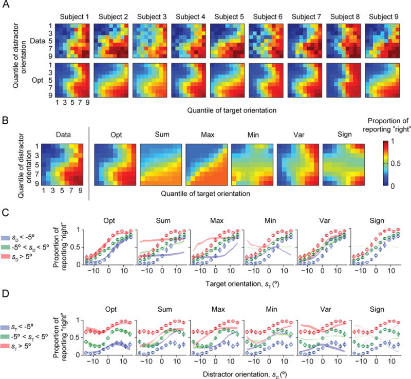
The Opt model fits better than the heuristic models. (A) Proportion of reporting “right” (color) as a function of target and distractor orientation quantiles, for individual subjects. The top plot shows the data, the top the fits of the Opt model. (B) As (A), averaged over subjects. The leftmost plot shows the data from Fig. 1C, the other plots the model fits. (C) Proportion of reporting “right” as a function of target orientation s_T. Circles and error bars: data; shaded areas: model fits. (D) Proportion of reporting “right” as a function of distractor orientation s_D.

Figure 7. Model comparison.

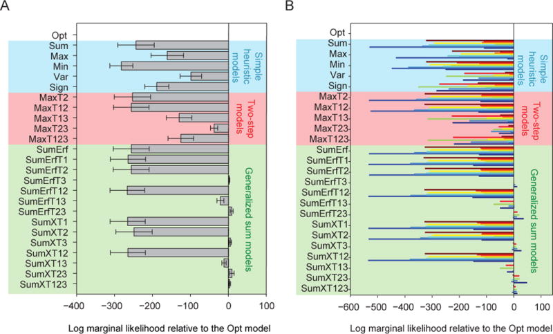
(A) Mean and s.e.m. across subjects of the difference in log marginal likelihood between each model and the Opt model. (B) Difference in log marginal likelihood between each model and the Opt model for individual subjects; bars of different colors represent different subjects.

Comparison between the optimal model and the two-step models

None of the two-step models fits the data well (Fig. 4A–C). Bayesian model comparison confirms this (Fig. 7A–B): the mean LML of the Opt model exceeds that of the two-step models by 253 ± 48, 256 ± 47, 130 ± 34, 38 ± 10 and 126 ± 34 (p < 0.01). The Opt model is more likely than any of the two-step models for all nine subjects (Fig. 7B). We obtained nearly identical results using the *IC information criteria (Fig. A2). This suggests that in perceptual decision-making, human observers do not follow the heuristic of only relying on the most discriminative cue.

Figure 4. Model fits of the two-step models.

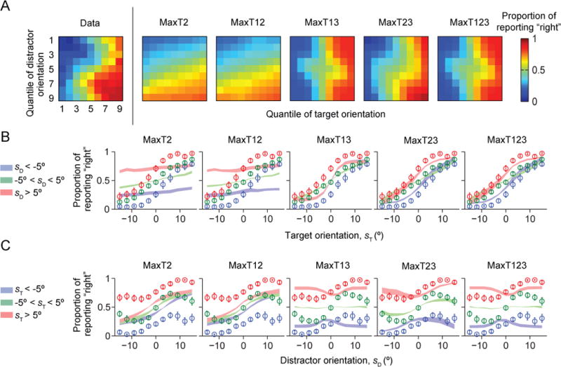
The Opt model fits better than the two-step models. (A) Proportion of reporting “right” (color) as a function of target and distractor orientation quantiles, averaged over subjects. The leftmost plot shows the data from Fig. 1C, the other plots the model fits. (B) Proportion of reporting “right” as a function of target orientation s_T. Circles and error bars: data; shaded areas: model fits. (C) Proportion of reporting “right” as a function of distractor orientation s_D.

Comparison between the optimal model and the generalized sum models

So far, none of the simple models tested can account for human behavior. Among the “generalized sum models”, those without the distractor variance term (Term 3) fitted poorly to human data (Figs. 5–6). The LML of the Opt model was higher than the log likelihoods of the models without Term 3 by 256 ± 47 (SumErf), 265 ± 46 (SumErfT1), 256 ± 47 (SumErfT2), 266 ± 46 (SumErfT12), 266 ± 46 (SumXT1), 249 ± 48 (SumXT2), and 265 ± 46 (SumXT12) (p < 0.001; Fig. 7A–B). However, models that included Term 3 were not distinguishable from the Opt model: the LML differences were −1.9 ± 1.3 (SumErfT3; p = 0.22), 21.7 ± 9.1 (SumErfT13; p=0.05), −8.2 ± 4.1 (SumErfT23; p = 0.10), −4.8 ± 3.3 (SumXT3; p = 0.20), 12.2 ± 5.7 (SumXT13; p = 0.08), −8.9 ± 5.8 (SumXT23; p = 0.19), and −3.1 ± 2.1 (SumXT123; p = 0.20). We obtained nearly identical results using the *IC information criteria (Fig. A2). Thus, like in the synthetic data used for model recovery, seven suboptimal models (SumErfT3, SumErfT13, SumErfT23, SumXT3, SumXT13, SumXT23, and SumXT123) fitted the data about as well as the Opt model. However, these are by no means simple models (Table 1). Our results suggest that the distractor variance term (Term 3) is a crucial component of the decision rule, implying that subjects used the knowledge that the three distractors have the same orientation in their decision.

Figure 5. Model fits of the generalized sum models of the SumErfT* type.

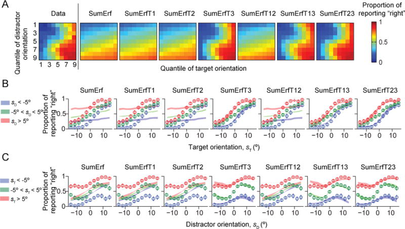
Models contain term 3 (SumErfT3, SumErfT13, and SumErfT23) fit about as well as the Opt model. (A) Proportion of reporting “right” (color) as a function of target and distractor orientation quantiles, averaged over subjects. The leftmost plot shows the data from Fig. 1C, the other plots the model fits. (B) Proportion of reporting “right” as a function of target orientation s_T. Circles and error bars: data; shaded areas: model fits. (C) Proportion of reporting “right” as a function of distractor orientation s_D.

Figure 6. Model fits of generalized sum models of the SumXT* type.

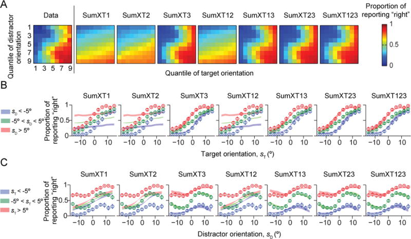
Models contain term 3 (SumXT3, SumXT13, SumXT13, and SumXT123) fit about as well as the Opt model. (A) Proportion of reporting “right” (color) as a function of target and distractor orientation quantiles, averaged over subjects. The leftmost plot shows the data from Fig. 1C, the other plots the model fits. (B) Proportion of reporting “right” as a function of target orientation s_T. Circles and error bars: data; shaded areas: model fits. (C) Proportion of reporting “right” as a function of distractor orientation s_D.

Model agreement

We found that seven (out of 24) suboptimal models can describe human behavior equally well as the Opt model. This might seem unsatisfactory, because it seems no definite conclusion can be drawn about whether people are optimal or not. Here, we argue that it is flawed to think of the distinction between optimal and suboptimal models as categorical, and that the seven well-fitting suboptimal models are for all practical purposes identical to the Opt model. A first hint of this was provided by the earlier model recovery analysis, in which we found that models within this group of eight models are indistinguishable (Fig. A1). However, we can quantify similarity between models in more detail. We will do this in two ways.

One way to think of model similarity is in terms of predicted accuracy. We computed the proportion correct predicted by different models given the same set of simulated stimulus vectors (consisting of 100,000 trials) across a range of values of the noise parameter σ (0.01 to 10 with a step of 0.01). We found that the accuracy levels predicted by these eight models are nearly identical (Fig. 8A), which means that observers using any of these eight decision rules would all obtain near-maximal accuracy.

Figure 8. Model similarity and goodness of fit.

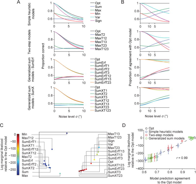
(A) Proportion correct as a function of the noise level σ for all models. (B) Proportion of trials for which a model makes the same prediction as the Opt model, as a function of σ. (C) Averaged prediction agreement (“Agreement”) visualized using multi-dimensional scaling. Each dot represents a model, and the distance between two models represents the disagreement between those models. The color of a dot represents its log marginal likelihood. Models that agree more with the Opt model tend to have a higher log marginal likelihood. (D) Mean (open circle) and s.e.m. (error bar) across subjects of a model’s log marginal likelihood as a function of its Agreement with the Opt model. Each dot indicates a model. The solid line represents the best linear fit. r is the Pearson correlation.

This analysis still leaves two possibilities: the seven alternative models do well because they are nearly identical to the Opt model in their trial-to-trial predictions, or because they account better than the Opt model for some trials and worse for others. In other words, we are not just interested in whether an observer uses a rule that allows near-maximal accuracy for a given noise level, but also in whether they use the specific decision rule Eq. (5).

To distinguish between these possibilities, we examined the trial-to-trial agreement between the model predictions of the Opt model and of each alternative model, under a lapse rate of zero. (A nonzero lapse rate would simply replace some responses by coin flips and is therefore uninteresting.) At each value of the noise level σ, we simulated 100,000 measurement vectors drawn from the generative model. For each measurement vector, the Opt and the alternative model made a deterministic prediction for the binary response. Comparing these predictions across all measurement vectors, we obtain a “proportion agreement”. We then plotted this quantity as a function of the noise level σ (Fig. 8B). The seven models that were indistinguishable from the Opt model made trial-to-trial predictions that agreed with those of the Opt model on more than 95% of trials. This shows that the models that fit about as well as the Opt model do so because the predictions of these models and the Opt model strongly agree from trial to trial.

A structure on the space of decision rules?

Although we tested many more models than is common in psychophysics studies, the set of all possible models is obviously infinite, which make it hard to infer whether an untested model would fit better. However, we are in the special circumstance that our models only differ in their decision rules. Here, we make use of this property to explore the structure of the decision rule space, with the goal of making inferences beyond the decision rules we tested.

In our task, a decision rule is a mapping from a measurement vector $\mathbf{x}\in {ℝ}^4$ and the parameter σ to a binary response $\widehat{C}=\pm 1$. There are infinitely many such mappings; when we fix σ, one can think of them as different ways of dividing four-dimensional space into black and white regions (for a three-dimensional analog showing the decision boundary, see Fig. 2B). One could shrink the space of decision rules by imposing that d must be antisymmetric under the sign flip $\mathbf{x}\mapsto -\mathbf{x}$, and invariant under permutations of the elements of x. In addition, one could impose smoothness constraints or neural constraints. Even so, d-space will still be infinite-dimensional and will not be a vector space in an obvious way. However, it is possible to equip it with a metric structure, which we will describe now.

In the previous section, we introduced the proportion of trial-to-trial agreement between two decision rules. There, it was a function of σ, but we can reduce it to a single number by averaging over σ:

$$\text{Agreement}(d_1,d_2)={\langle {\delta }_{d_1(\mathbf{x},\sigma ),d_2(\mathbf{x},\sigma )}\rangle }_{\mathbf{x},\sigma }.$$ (12)

In this equation, δ denotes the Kronecker delta function, which equals 1 when its two subscripted integer arguments are equal to each other and 0 otherwise. The average 〈…〉 is over everything: noise realizations, stimuli, and the parameter σ (for which we again use the range (0,10]). Agreement is linearly related to the Hamming distance (Hamming, 1950) computed across the two binary strings of $\widehat{C}$ values obtained by evaluating both decision rules on randomly sampled (σ, x) pairs. Incidentally, this means that Agreement equips the space of decision rules with a metric structure.

The Agreement metric is less general than Kullback–Leibler (KL) or Jensen-Shannon (JS) divergence: Agreement is designed for comparing two deterministic decision rules acting on the same internal representation, whereas the divergences can be used to characterize similarity between any two models. However, Agreement has the advantage of capturing the trial-to-trial similarity between model predictions: while the divergences only compare the predicted distributions of responses conditioned on the stimuli, s, Agreement compares the predicted individual responses conditioned on the internal representation x. Consider an example in which a specific stimulus s is repeated many times, and two models A and B both predict the subject to report “right” on 70% of these trials. Then, KL/JS divergence between A and B will be 0. However, Agreement between A and B might differ greatly. One extreme possibility is that A and B make the exact same prediction for every x that is generated from s, that is, Agreement is 100%. The other extreme possibility is that A and B make maximally distinct predictions; in this case, Agreement is only 40%.

Relation between Agreement with Opt and goodness of fit

Now that we have used Agreement to define a structure on model space, we can examine how goodness of fit (log marginal likelihood, or LML) depends on Agreement. As a first step, we visualized the space of decision rules using multi-dimensional scaling. This method converts the matrix of Agreement values between pairs of decision rules (25×24/2=300 values in total) into distances in a low-dimensional space (Borg & Groenen, 2005). We found that the models that lie farther away from the Opt model in this low-dimensional space tend to fit worse (Fig. 8C). This suggests that Agreement is informative about goodness of fit. We now examine this suggestion in more detail.

Given a data set, an ideal conclusion to draw would be that one particular decision rule, say d*, has the highest LML in the space of all plausible mappings d. In practice, we can only test a small number of d, so it is helpful to know whether there exists a monotonic relationship between LML and Agreement with d*. In fact, a sufficient condition for d* being the only maximum in all of d-space is that LML is lower whenever Agreement to d* is lower. The LML landscape does not necessarily obey this property globally, and is in fact unlikely to; for example, there could be local maxima (multimodality) or ridges. However, the property might still hold in most of the d-space, and therefore we think that the correlation between LML and Agreement (CLA) is informative.

Across the 25 models we tested, we find that a model’s LML is strongly correlated with its Agreement with the Opt model, with a correlation of 0.99 (Fig. 8D). The correlation was much lower when we correlated LML with the Agreement with a model other than Opt, except for the seven other best models (Fig. 9A, Fig. A3). These observations suggest that the more similar a model’s lapse-free trial-to-trial predictions are to the eight best models, the better the model (with a lapse rate) fits the human data.

Figure 9. Correlation between log marginal likelihood and Agreement (CLA) as a potential measure of the global maximum of goodness of fit in model space.

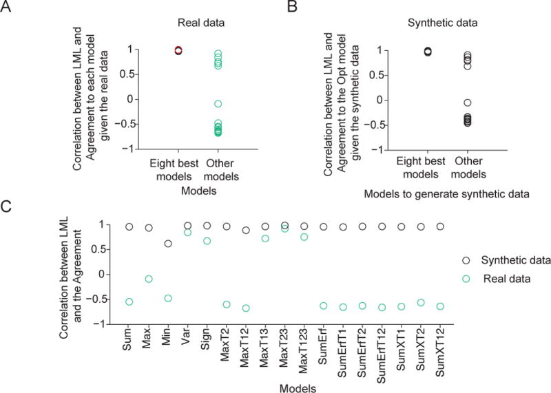
(A) Agreement, and therefore CLA, is computed relative to a reference model. CLA is high when the reference model is the Opt model (red circle, see also Fig. 8D) or one of the seven other best models (see also Fig. A3). CLA is significantly lower when the reference model is a different model (Wilcoxon rank-sum test, p = 8.4×10⁻⁵). (B) Given synthetic data generated from one of the eight best models, CLA with the Opt model as the reference is high. Given synthetic data generated from a model outside of the eight best, CLA with the Opt model as the reference is significantly lower (Wilcoxon rank-sum test, p = 8.4×10⁻⁵, see also Fig. A4). This serves as a negative control for the high CLA with the Opt model as a reference (red circle in (A) and Fig. 8D). (C) Given synthetic data generated from any one model, the CLA with that model as the reference is high (> 0.9). Moreover, given synthetic data generated from a model outside of the eight best, the CLA with that model as a reference is significantly higher than given the real data (Wilcoxon signed-rank test, p = 2.9×10⁻⁴, see also Fig. A5). This serves as a positive control for the low CLAs with the models outside of the eight best as reference models (green circles in (A)).

In synthetic data generated using parameters fitted to subject data (see “Model recovery”), CLA with the Opt model as the reference model was only high when the data were generated from the seven other best models (Fig. 9B, Fig. A4). Moreover, the CLA with a specific model as the reference model was high when the synthetic data were generated using that model (Fig. 9C, Fig. A5). Therefore, the observed high correlation between a model’s LML on subject data and its Agreement with one of the eight best models is consistent with the eight best models being close to the true model underlying the data.

However, this argument relies on the small, rather arbitrary, and possibly biased set of models that we tested here. In particular, the high correlation would be unsurprising if the models tested all reside in a local neighborhood of the Opt model. In addition, a drawback of the analysis above is that Agreement was defined on models without a lapse rate, whereas LML was computed on the same models with a lapse rate. To further investigate how close the eight best models are to the true model underlying the data, we now introduce an independent approach.

HOW GOOD ARE THE BEST MODELS?

Here we use an information-theoretical method to determine how well a model fits in an “absolute” sense, specifically, how much room there is for an untested model to fit better than the eight best models. The basic idea can be illustrated with a simple example: if a biased coin has a probability p of coming up heads, and we try to account for the outcomes of N independent tosses of that coin, then the best we can do is to state for each toss that the probability of heads is p. When N is large, the log likelihood of this model will be the sum of Np log p (from the heads outcomes) and N(1−p) log (1−p) (from the tails outcomes), which is the negative entropy of a sequence of this coin’s toss outcomes. No model can have a higher log likelihood: the log likelihood of any model is bounded from above by the pure stochasticity of the data. The argument below amounts to estimating how close the log likelihood of our best models is to the upper bound given by the negative entropy.

Kullback-Leibler divergence

The data D produced by a model M follow a probability distribution p(D|M). If we assume that there is a true model M_true, then its data distribution is p(D|M_true). A principled measure of the distance between a model M and the true model M_true is the Kullback-Leibler divergence between these two data distributions (Cover & Thomas, 2005):

$$D_{\text{KL}}\left(p\left(D|M_{\text{true}}\right)\Vert p\left(D|M\right)\right)\equiv {\displaystyle \sum _{D}p\left(D|M_{\text{true}}\right)}\log \frac{p\left(D|M_{\text{true}}\right)}{p\left(D|M\right)}.$$

This quantity is always non-negative and can be evaluated as:

$$D_{\text{KL}}\left(p\left(D|M_{\text{true}}\right)\Vert p\left(D|M\right)\right)=-H\left(p\left(D|M_{\text{true}}\right)\right)+H\left(p\left(D|M_{\text{true}}\right),p\left(D|M\right)\right),$$ (13)

where

$$H\left(p\left(D|M_{\text{true}}\right)\right)=-{\displaystyle \sum _{D}p\left(D|M_{\text{true}}\right)}\log p\left(D|M_{\text{true}}\right)$$ (14)

is the entropy of the data distribution p(D|M_true), and

$$H\left(p\left(D|M_{\text{true}}\right),p\left(D|M\right)\right)=-{\displaystyle \sum _{D}p\left(D|M_{\text{true}}\right)}\log p\left(D|M\right)$$ (15)

is the cross-entropy between p(D|M_true) and p(D|M), and, as we will see below, closely related to model log likelihood. Since D_KL is non-negative, the negative entropy is an upper bound on the negative cross-entropy. The KL divergence corresponds to unexplained variation, the entropy to subject stochasticity (“unexplainable variation”), and the negative cross-entropy to the goodness of fit (“explained variation”). Thus, goodness of fit, KL divergence, and unexplainable variation sum up to a perfect fit (zero). No model can fit the data better than allowed by the stochasticity of subject responses.

Both terms in Eq. (13) involve a sum over all possible data sets D generated from model M_true, but we have only a single one available, namely the subject data. Therefore, both terms have to be estimated based on that one data set, which we denote by “data”, as before. Before we resolve this issue, we will first simplify Eqs. (14) and (15) by assuming independence of trials and discretizing the stimuli.

Negative entropy term

A possible data set consists of a binary vector of length Ntrials, consisting of +1 and −1 responses: $D=\widehat{\mathbf{C}}\in {\left\{\pm 1\right\}}^{N_{\text{trials}}}$. We now assume that the trials are conditionally independent of each other. We can then evaluate the negative entropy of p(D|M_true), starting from Eq. (14):

$$\begin{array}{l}-H\left(p\left(\widehat{C}|M_{\text{true}}\right)\right)={\displaystyle \sum _{\widehat{C}\in {\left\{\pm 1\right\}}^{N_{\text{trials}}}}p\left(\widehat{C}|M_{\text{true}}\right)\log p\left(\widehat{C}|M_{\text{true}}\right)}\\ ={\displaystyle \sum _{{\widehat{C}}_1=\pm 1}\dots {\displaystyle \sum _{{\widehat{C}}_{N_{\text{trials}}}=\pm 1}\left({\displaystyle \coprod _{i=1}^{N_{\text{trials}}}p\left({\widehat{C}}_i|M_{\text{true}}\right)}\right)}}\log \left({\displaystyle \prod _{i=1}^{N_{\text{trials}}}p\left({\widehat{C}}_i|M_{\text{true}}\right)}\right),\\ ={\displaystyle \sum _{i=1}^{N_{\text{trials}}}{\displaystyle \sum _{{\widehat{C}}_i=\pm 1}p\left({\widehat{C}}_i|M_{\text{true}}\right)}}\log p\left({\widehat{C}}_i|M_{\text{true}}\right)\end{array}$$

where ${\widehat{C}}_i$ is the subject’s response on the i^th trial.

To make further progress, we need to define unique stimulus conditions that have sufficiently many trials. To this end, we binned the data as in Fig. 1B: 9 quantiles for s_T crossed with 9 quantiles for s_D. We denote the number of trials when the stimuli are in the j^th stimulus bin (j=1,…, 81) by N_j, and, among those, the number of trials when the subject responded “right”, by n_j. Thus, we reduce each subject’s data to 81 counts. We verified that the number of bins did not meaningfully affect our results.

Using this discretization, the distribution $p\left({\widehat{C}}_i|M_{\text{true}}\right)$ is the same for all trials i in the same stimulus condition. Therefore, we can group the trials by stimulus bin j, and negative entropy becomes

$$-H\left(p\left(\widehat{C}|M_{\text{true}}\right)\right)={\displaystyle \sum _{j=1}^{81}{N}_j}{\displaystyle \sum _{{\widehat{C}}_j=\pm 1}p\left({\widehat{C}}_j|M_{\text{true}}\right)}\log p\left({\widehat{C}}_j|M_{\text{true}}\right).$$

Defining ${\pi }_j\equiv p\left({\widehat{C}}_j=1|M_{\text{true}}\right)$, we have

$$\begin{array}{|c|}\hline -H\left(p\left(\widehat{C}|M_{\text{true}}\right)\right)={\displaystyle \sum _{j=1}^{81}{N}_j}\left({\pi }_j\log {\pi }_j+\left(1-{\pi }_j\right)\log \left(1-{\pi }_j\right)\right).\\ \hline\end{array}$$ (16)

Negative cross-entropy term

We now turn to the cross-entropy of p(D|M_true) and p(D|M), as given by Eq. (15). This term is difficult to estimate, because responses in different stimulus bins are independent only conditional on the parameters. Unfortunately, the parameters θ (J and λ) are unknown and have to be estimated from the data or marginalized over. Here, the former is easier. For each model, we used every other trial to obtain maximum-likelihood estimates $\widehat{\theta }$ of the parameters (using the same parameter grid as before), and then used these values to evaluate model predictions on the other half of the trials. Then, we can use a trial factorization and stimulus binning analogous to the ones done above for the entropy, to arrive at

$$\begin{array}{|c|}\hline -H\left(p\left(\widehat{\mathbf{C}}|M_{\text{true}}\right),p\left(\widehat{\mathbf{C}}|M,\widehat{\theta }\right)\right)={\displaystyle \sum _{j=1}^{81}{N}_j}\left({\pi }_j\log p\left({\widehat{\mathbf{C}}}_j=1|M,\widehat{\theta }\right)+\left(1-{\pi }_j\right)\log p\left({\widehat{C}}_j=-1|M,\widehat{\theta }\right)\right).\\ \hline\end{array}$$ (17)

where $p\left({\widehat{C}}_j|M,\widehat{\theta }\right)$ denotes the probability of response ${\widehat{C}}_j$ under model M on a trial on which the stimuli are in the j^th bin. In practice, we computed the latter values as a weighted average of the proportions of ${\widehat{C}}_j$ across a fine grid of stimulus combinations in the j^th bin, with weights given by the probabilities of those stimulus combinations.

Estimating the terms: deviance approach

We now have expressions for the two terms in the KL divergence under the trial factorization and stimulus binning, Eqs. (16) and (17). The KL divergence is the difference between these two quantities. In computing this, we face a problem: {π_j}, the predicted proportion of ${\widehat{C}}_j=1$ responses under the true model, are unknown because the true model is unknown. We will first describe the standard way to deal with this problem, then our way.

The standard way to deal with the problem that {π_j}are unknown is to estimate them as the empirical proportions of ${\widehat{C}}_j=1$ responses, in other words, as ${\widehat{\pi }}_j=\frac{n_j}{N_j}$. Then, the estimator of the negative entropy becomes

$$-\widehat{H}\left(p\left(\widehat{\mathbf{C}}|M_{\text{true}}\right)\right)={\displaystyle \sum _{j=1}^{81}{N}_j}\left({\widehat{\pi }}_j\log {\widehat{\pi }}_j+\left(1-{\widehat{\pi }}_j\right)\log \left(1-{\widehat{\pi }}_j\right)\right)$$ (18)

and the estimator of the negative cross-entropy becomes

$$-\widehat{H}\left(p\left(\widehat{\mathbf{C}}|M_{\text{true}}\right),p\left(\widehat{\mathbf{C}}|M,\widehat{\theta }\right)\right)={\text{LL}}_{\text{cv}}\left(M\right),$$ (19)

where

$$L{L}_{\text{cv}}\left(M\right)\equiv {\displaystyle \sum _{j=1}^{81}\left(n_j\log p\left({\widehat{C}}_j=1|M,\widehat{\theta }\right)+\left(N_j-n_j\right)\log p\left({\widehat{C}}_j=-1|M,\widehat{\theta }\right)\right)}$$ (20)

is the cross-validated log likelihood of model M (compare Eq. (10)). The difference between these two terms is then the estimator of KL divergence:

$${\widehat{D}}_{\text{KL}}\left(p\left(D|M_{\text{true}}\right)\Vert p\left(D|M\right)\right)={\displaystyle \sum _{j=1}^{81}{N}_j}\left({\widehat{\pi }}_j\log \frac{{\widehat{\pi }}_j}{p\left({\widehat{C}}_j=1|M,\widehat{\theta }\right)}+\left(1-{\widehat{\pi }}_j\right)\log \frac{1-{\widehat{\pi }}_j}{p\left({\widehat{C}}_j=-1|M,\widehat{\theta }\right)}\right)$$

Up to an irrelevant factor of 2, this is also known as the deviance (Wichmann & Hill, 2001). It is common to perform a statistical test on the deviance to determine whether it is significantly different from 0. If it is not, then the model is statistically “as good as possible”.

Although such an analysis of deviance is widespread, it suffers from a fundamental problem: ${\widehat{\pi }}_j=\frac{n_j}{N_j}$ is an unbiased estimator of π_j, but ${\widehat{\pi }}_j$ log ${\widehat{\pi }}_j$ is not an unbiased estimator of π_j log π_j. In fact, the bias in estimating entropy has been characterized in detail (Grassberger, 1988, 2003). Therefore, we explore a different solution here.

Estimating the terms: new approach

Negative entropy term

To estimate the negative entropy, we use the Grassberger estimator (Grassberger, 2003), evaluated on the same half of the data as used to estimate the cross-entropy:

$$-\widehat{H}\left(p\left(D|M_{\text{true}}\right)\right)=-{\displaystyle \sum _{j=1}^{81}{N}_j}\left(G_{N_j}-\frac{1}{N}\left(n_j{G}_{n_j}+\left(N_j-n_j\right)G_{N_j-n_j}\right)\right),$$ (21)

where the numbers G_n are obtained through G₀=0, G₁=−γ–log 2 (where γ = 0.577215…is Euler’s constant), G₂=2−γ–log 2,, and for n ≥ 1, G_2n+1=G_2n and $G_{2n+2}=G_{2n}+\frac{2}{2n+1}$. Thus, $G_{2n}=-\gamma -\log 2+\frac{2}{1}+\frac{2}{3}+\frac{2}{5}+\frac{2}{2n+1}.$

Negative cross-entropy term

The negative cross-entropy term is linear in π_j and therefore does not suffer from the same biased estimation problem. Therefore, we use the estimator of Eq. (19), $-\widehat{H}\left(p\left(\widehat{\mathbf{C}}|M_{\text{true}}\right),p\left(\widehat{\mathbf{C}}|M,\widehat{\theta }\right)\right)={\text{LL}}_{\text{cv}}\left(M\right).$

KL divergence

Our estimator of the KL divergence is then the difference of Eqs. (21) and (19):

$$\begin{array}{|c|}\hline {\widehat{D}}_{\text{KL}}\left(p\left(D|M_{\text{true}}\right)\Vert p\left(D|M\right)\right)=-{\widehat{H}}_{\mathrm{G}}\left(p\left(D|M_{\text{true}}\right)\right)-{\text{LL}}_{\text{cv}}\left(M\right).\\ \hline\end{array}$$ (22)

Significance testing

To test whether D_KL is significantly greater than 0, we can no longer assume a chi-squared distribution, as is common for establishing significance of deviance (Collett, 2002, sects 3.8; Wichmann & Hill, 2001). In fact, we do not know how to compute a confidence interval on the expression in Eq. (22). Therefore, we make a further approximation by regarding our Grassberger estimate of negative entropy as the truth, and only computing a confidence interval on the cross-entropy term. This can lead to false alarms (a model is falsely declared as being substantially different from the truth) but not to misses; thus, it is a conservative approach if we aim to test whether our best models are indistinguishable from the truth.

To compute a confidence interval for the cross-entropy, we use a Bayesian approach (i.e. we compute a credible interval), i.e. we compute the posterior probability distribution over Eq. (17). First, we compute the posterior over π_j assuming a flat prior; a Jeffreys’ prior would not substantially change our results. Then, the posterior over π_j is a beta distribution with mean $\frac{n_j}{N_j}$ and variance $\frac{(n_j+1)(N_j-n_j+1)}{{(N_j+2)}^2(N_j+3)}$. The next step is to approximate the beta distribution with a normal distribution with the same mean and variance, and make use of the independence of the π_j. Then, the posterior over $-H\left(p\left(\widehat{\mathbf{C}}|M_{\text{true}}\right),p\left(\widehat{\mathbf{C}}|M,\widehat{\theta }\right)\right)$ has mean LL_cv as before (Eq. (20)), and variance

$${{\displaystyle \sum _{j=1}^{81}\left(N_j\log \frac{p_j\left(\widehat{C}=1|M,\widehat{\theta }\right)}{p_j\left(\widehat{C}=-1|M,\widehat{\theta }\right)}\right)}}^2\frac{\left(n_j+1\right)\left(N_j-n_j+1\right)}{{\left(N_j+2\right)}^2\left(N_j+3\right)}.$$ (23)

This yields a 95% credible interval of the estimate of the KL divergence:

$$\left[\begin{array}{l}-\widehat{H}\left(p\left(D|M_{\text{true}}\right)\right)-{\text{LL}}_{\text{cv}}\left(M\right)-1.96\cdot \sqrt{\text{var}\left({\text{LL}}_{\text{max}}\left(M\right)\right),}\hfill \\ -\widehat{H}\left(p\left(D|M_{\text{true}}\right)\right)-{\text{LL}}_{\text{cv}}\left(M\right)+1.96\cdot \sqrt{\text{var}\left({\text{LL}}_{\text{max}}\left(M\right)\right)}\hfill \end{array}\right].$$ (24)

For every subject, we computed: the LL_max of a random coin-flip model (−N_trials·0.5 log 2), the Grassberger estimate of negative entropy (Eq. (21)), LL_cv(M) for all models, and the 95% credible interval of the estimate of the negative cross-entropy for the Opt model (Eq.(24)) (Fig. 10, Table 2). For most subjects, the estimate of negative cross-entropy is lower than the estimate of negative entropy; for two subjects, they are reversed. Since it is mathematically impossible for negative cross-entropy to exceed the negative entropy, this is an indication of estimation error. For eight out of nine subjects, the negative entropy was not significantly higher than the negative cross-entropy of the Opt model, indicating that the Opt model fits the data very well in an “absolute” sense (Table 2). The same applies to the seven models that are indistinguishable from the Opt model (see Table A2).

Figure 10. Information-theoretical estimate of how good the eight best models are.

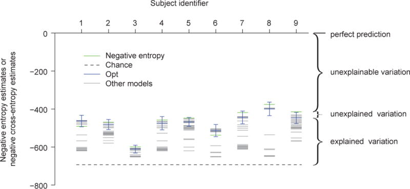
Each column represents a subject. For each subject, the green line represents an estimate of the negative entropy of the data, the dashed black line the negative cross-entropy between a coin-flip model and the true model, the blue line an estimate of the negative cross-entropy between the Opt model and the true model, and the grey lines estimates of the negative cross-entropies between other models and the true model. The error bar represents an estimate of the 95% credible interval of the negative cross-entropy between the Opt model and the true model. The estimate of the negative cross-entropy between the Opt model and the true model is not significantly different from the estimate of the negative entropy of the data (one-sided Wilcoxon signed-rank test, p = 0.15), suggesting that the Opt model explains most of the explainable variation. The same holds for the seven other best models (see main text).

Table 2.

For each subject, we show the estimated negative entropy, the corresponding estimated upper bound on the prediction accuracy of any model, the estimated 95% confidence interval of the negative cross-entropy of the Opt model, and the corresponding confidence interval of prediction accuracy. The p value is the estimated probability that the negative cross-entropy is equal to or higher than the negative entropy (with higher being theoretically impossible).

ID	Negative entropy	Prediction accuracy upper bound	95% CI of negative cross-entropy of Opt	95% CI of prediction accuracy of Opt	95% CI of DKL	p value
1	−492	0.61	[−494, −433]	[0.61, 0.65]	[−59, −2]	0.97
2	−470	0.63	[−508, −455]	[0.60, 0.63]	[−15, 38]	0.20
3	−599	0.55	[−632, −590]	[0.53, 0.55]	[−9, 33]	0.14
4	−458	0.63	[−510, −440]	[0.60, 0.64]	[−18, 52]	0.17
5	−448	0.64	[−491, −444]	[0.61, 0.64]	[−4, 43]	0.05
6	−537	0.58	[−545, −482]	[0.58, 0.62]	[−55, 8]	0.92
7	−419	0.66	[−478, −411]	[0.62, 0.66]	[−8, 59]	0.07
8	−376	0.69	[−435, −364]	[0.64, 0.69]	[−8, 59]	0.10
9	−414	0.66	[−476, −418]	[0.62, 0.66]	[4, 64]	0.02

Across subjects, the mean KL divergence between the Opt model and the true model is not significantly greater than 0 (p = 0.15, one-sided Wilcoxon signed-rank test), confirming that the Opt model explains most of the explainable variation. The same is true for the seven other best models (SumErfT3: p = 0.25, SumErfT13: p = 0.13, SumErfT23: p = 0.25, SumXT3: p = 0.21, SumXT13: p = 0.13, SumXT23: p = 0.18, SumXT123: p = 0.21).

We can restate the comparison between negative cross-entropy and negative entropy in perhaps more intuitive terms. The negative cross-entropy, when divided by the number of trials and then exponentiated, represents the geometric mean probability of the model correctly predicting the subject’s response on a given trial. Similarly, the negative entropy divided by the number of trials and exponentiated represents the geometric mean probability of correctly predicting the subject’s response on a given trial given the empirical response frequencies. For example for the Opt model, the prediction accuracy values are 0.63±0.01 and 0.62±0.01, respectively (for individual subjects, see Table 2). This means that the Opt model predicts about as well as possible based on random variability in the data. Taken together, these results show that there is relatively little room for an untested model to fit better than our eight best models.

In summary, we so far have used two approaches to infer the models in the model space beyond the models we tested. Both approaches support the conclusion that the Opt model and the seven other best models are close to the true model.

EXPERIMENT 2: IMPLICIT REPRESENTATION OF UNCERTAINTY

Although the Opt decision rule was derived using the principles of Bayesian inference, our finding that the rule describes human behavior well does not imply that people reason with probabilities. In particular, an observer can, through the trial-to-trial feedback provided in the experiment, learn the Opt rule as a policy or look-up table, without ever representing probabilities in their brain. In earlier work, we therefore distinguished optimal computation from probabilistic computation (Ma, 2012). In the latter, the observer uses an implicit representation of sensory uncertainty, or even of an entire probability distribution over a sensory stimulus, in downstream computation. There is substantial evidence that people do this (for a review, see Ma & Jazayeri, 2014) but not much from tasks in which the decision rules is as complicated as here.

To vary uncertainty, one can vary stimulus reliability. In Experiment 2, we determined whether people are optimal when we train them at high stimulus reliability and test at low stimulus reliability. This test is a special case of “Bayesian transfer”, a term coined by Maloney and Mamassian (Maloney & Mamassian, 2009) to indicate that a truly probabilistic Bayesian observer should maintain priors, likelihoods, and cost functions as building blocks that can be mixed and matched according to the task demands; the experimental prediction is that people should generalize nearly immediately to a new prior, likelihood, or cost function and combined with other components that they learned previously. In our case, we generalize from a narrow likelihood function (high stimulus reliability) to a wide one (low stimulus reliability).

Methods

Experiment 2 was identical to Experiment 1 except for the following differences. The experiment consisted of three sessions, held on different days. Each session contained 6 blocks of 150 trials each. During the instruction phase on the first day, subjects viewed a plot of the Gaussian orientation distribution p(s) for a single item (not conditioned on C); the meaning of this plot was explained to them using vocabulary that matched their background. Subjects also viewed 30 stimuli whose orientations were drawn from p(s).

Blocks 1 and 4 of each session were training blocks, in which the stimuli were presented at high contrast (peak luminance of the Gabor patch: 120 cd/m²), and correctness feedback was provided after each trial. The other blocks were testing blocks. The stimuli in these blocks had lower contrast (peak luminance: 56 cd/m²) and no feedback was provided. Five subjects (3 female) participated in Experiment 2; all subjects were naïve to the experiment.

The instruction and training were meant to make the subjects to learn the stimulus distributions and correct any biases on left/right reporting, which are the same in both training and testing trials. However, the likelihood functions on the testing trials could not be learned from the training trials, because the stimuli had different reliability.

Results

We performed the same analysis as in Experiment 1 on the testing trials of Experiment 2. We found that the Opt model is still among the best-fitting models (Fig. 11A–B) and Bayesian model comparison revealed model rankings consistent with Experiment 1 (Fig. 11C–D). The Opt model and the seven other best models from Experiment 1 have higher LML than the other models.

Figure 11. Results of Experiment 2, in which feedback was withheld.

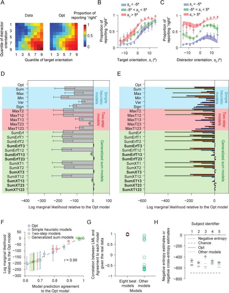
(A) Proportion of reporting “right” (color) as a function of each combination of target and distractor orientation quantiles (1 to 9), averaged over all 5 subjects. The left plot shows the data, the right the fits of the Opt model. (B) Proportion of reporting “right” as a function of target orientation. Circles and error bars: data; shaded areas: Opt model fits. (C) Proportion of reporting “right” as a function of distractor orientation. (D) Mean and s.e.m. across subjects of the log marginal likelihood of each model relative to the Opt model. Shades of different colors indicate the category of a model. (E) Log marginal likelihood of each model minus that of the Opt model, for individual subjects. In the bar plots, each color represents a different subject. (F) As Fig. 8D, for Experiment 2. (G) As Fig. 9A, for Experiment 2. CLA is high when the reference model is the Opt model (red circle) or one of the seven other best models, and significantly lower otherwise (Wilcoxon rank-sum test, p = 8.4×10⁻⁵). (H) As Fig. 10, for Experiment 2. The estimate of the negative cross-entropy between the Opt model and the true model is not significantly different from the estimate of the negative entropy of the data (one-sided Wilcoxon signed-rank test, p = 0.31), suggesting that the Opt model explains most of the explainable variation. The same conclusion holds for the seven other best models.

Moreover, the Agreement and information-theoretic analyses yield the same conclusions as in Experiment 1: a model’s LML is strongly correlated with its Agreement with the Opt model (r = 0.99, Fig. 11F), much less with its Agreement with a model outside of the best eight (Fig. 11G), our estimate of KL divergence between any of the eight best models and the true model is not significantly different from 0 (Fig. 11H; e.g., Opt: p = 0.31, one-sided Wilcoxon signed-rank test), and also hold for the seven other best models. These results suggest that the sensory uncertainty is internally represented and that people combine this information with the task demands to achieve near-optimal performance, instead of using a fixed policy or look-up table.

DISCUSSION

We tested the optimal decision rule against a series of suboptimal rules, including many simple heuristic rules, in a relatively complicated perceptual decision-making task involving multiple stimuli. We found that the optimal rule describes the rich patterns in human behavior extremely well, and better than the heuristic rules that we tested. Moreover, even without trial-to-trial feedback, the Opt model still provides the best fit, and the Opt model is still close to the true model in a absolute sense according to both the Agreement analysis and the KL divergence estimates, suggesting that the near-optimal behavior is not a result of establishing a look-up table through feedback, but a result of probabilistic computation.

It should be kept in mind that our model observer is not optimal in an absolute sense (Ma, 2012), because measurement noise is not zero. In fact, this noise itself might reflect suboptimality in earlier stages of processing (Pouget, Beck, Ma, & Latham, 2013), or attentional limitations (Mazyar, Van den Berg, & Seilheimer, 2013). Our notion of optimality pertains solely to the decision rule applied to noisy sensory information.

We found that seven suboptimal models fit the data as well as the Opt model. However, those models are indistinguishable from the Opt model both in a model recovery test and in trial-to-trial model agreement. This argues for dropping the hard distinction between optimal and suboptimal, and instead talking about “models indistinguishable from optimal”.

Although we tested a relatively large number of models, model space contains infinitely many more models. Therefore, we introduced and computed two quantities to estimate how well the Opt model and the seven other best models fit relative to untested models: a) the correlation across models between log marginal likelihood and trial-to-trial agreement with one of the best models, and b) an estimate of the KL divergence between the eight best models and the true model. The first approach defines a structure on the space of decision rules, but it only applies when decision rules are deterministic and act on the same internal representation. (However, it can likely be generalized by using KL divergence instead of Agreement.) The second approach is much more general, but involves many approximations. Taken together, however, we believe that we have provided evidence that it is difficult to find a rule that fits the data better than the Opt rule (and rules indistinguishable from it).

Although we were able to define “complexity” for our mathematically specified decision rules, the way in which we did so was rather arbitrary. Coming up with a general definition of the complexity of a mapping between internal representation and decision might be even more difficult, for several reasons. First, it is unclear how to define complexity when the decision rule does not admit a neat mathematical description, as is the case for MAP estimation when the task distributions are empirical (Griffiths & Tenenbaum, 2006). Second, a mathematically complex computational-level rule might be simple for neurons to implement, or conversely. For example, some complex optimization problems can be solved using “simple” network operations (Deneve, 2008; Hopfield & Tank, 1985; Hornik, Stinchcombe, & White, 1989; Nessler, Pfeiffer, Buesing, & Maass, 2013; Nessler, Pfeiffer, & Maass, 2008). These ambiguities in the meaning of the complexity or simplicity of a decision process pose as much of a challenge to those proposing simple heuristics as an organizing principle as they do to us. In fact, such ambiguities may make any debate between optimality and simplicity ill-defined. A better-defined broad question is in what task domains human behavior is indistinguishable from optimal.

Although it seems safe to claim that subjects are not always near-optimal in perceptual tasks, the evidence for that statement is surprisingly weak. First, apparent suboptimality can arise when there are many parameters to learn, the distributions are complex, the parameters vary greatly across trials (Landy, Goutcher, Trommershäuser, & Mamassian, 2007), or the subjects are not fully attending to a stimulus (Morales et al., 2015). However, when given a large number of training trials (Körding & Wolpert, 2004) or a real-life backstory (Seydell, McCann, Trommershäuser, & Knill, 2008), people exhibit near-optimal behavior even under those conditions. When subjects do not perfectly learn the parameters, the optimal model should take into account evolving posteriors over those parameters; subjects might then still be optimal given the limited information about the parameters they have available (Fiser, Berkes, Orbán, & Lengyel, 2010). Second, unexplained biases that seem suboptimal have been reported when people estimate the direction of moving dots (Jazayeri & Movshon, 2007; Rauber & Treue, 1998; Szpiro, Spering, & Carrasco, 2014); however, such biases might be due to the inhomogeneous nature of the tuning curves in the population encoding the stimulus (Wei & Stocker, 2015). Third, it has been suggested that people use a probability matching strategy, which is suboptimal (Wozny, Beierholm, & Shams, 2010). However, evidence in that study was mixed and somewhat indirect; in a direct comparison of probability matching and optimal estimation, the latter described human data better (Acuna, Berniker, Fernandes, & Kording, 2015). In our data, when we tested a probability matching version of the Opt model on our data, we found that its log likelihood is lower than that of the original Opt model by 73 ± 23 (Fig. 12), and that the original Opt model is more likely for all nine subjects. Fourth, in some domains of perception, heuristic models have historically been popular. An example is the maximum-of-outputs model in visual search (Nolte & Jaarsma, 1967). However, a review of studies in which that model did well showed that the optimal model described human data as well or better (Ma, Shen, Dziugaite, & Van den Berg, 2015). Thus, when we restrict ourselves to perceptual studies in which the generative model is well characterized, observers have fully learned the generative model, and proper model comparison has been performed, strong evidence for suboptimality in human behavior seems to be absent. Once recent challenge to this claim involved a task combining an uncertain perceptual judgment with a speeded reaching movement; the claim was there that subjects’ behavior obeyed a two-step model (Fleming et al., 2013). This needs to be explored further.

Figure 12. Comparison between probability matching version of the Opt model and the Opt model.

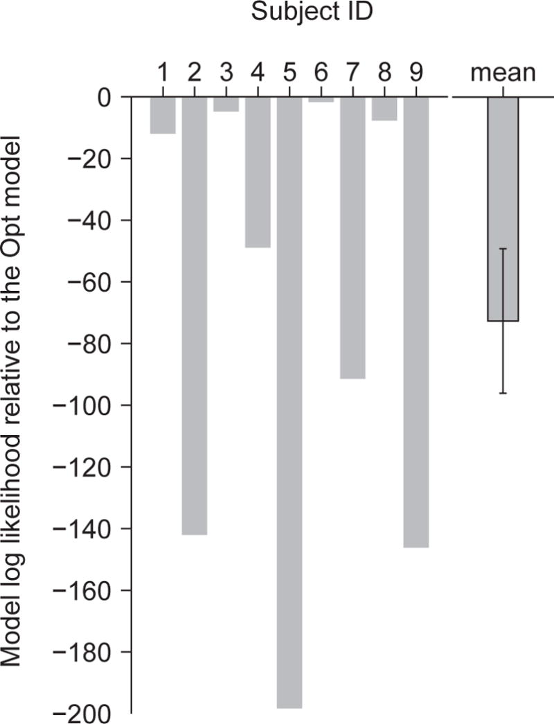
Difference in log marginal likelihood between the probability matching model and the Opt model for individual subjects. The last column shows the mean and s.e.m. of this difference.

What does our work imply for cognitive decision-making tasks? In some cases, such as predicting the weather, choosing a job, or playing chess, it might forever remain unknown whether people use near-optimal or simple rules, because both optimality and simplicity are hard to define, and people’s prior beliefs, computational constraints, and utility functions are unknown and very difficult to estimate. However, there is a rich arena of cognitive tasks that are restricted, parameterized, and allow for quantitative modeling. Examples include the learning of category boundaries (Ashby & Maddox, 2005), strategies for information gathering (Coenen, Rehder, & Gureckis, 2014; Steyvers, Tenenbaum, Wagenmakers, & Blum, 2003; Wason, 1960), estimation of everyday quantities (Griffiths, Chater, Kemp, Perfors, & Tenenbaum, 2010), category-based induction (Osherson, Smith, Wilkie, López, & Shafir, 1990), and intuitive physics (Battaglia, Hamrick, & Tenenbaum, 2013). In all these realms, it is possible and important to develop large numbers of plausible suboptimal, simple models and perform analyses similar to the ones we did here. This is, however, rarely done (Bowers & Davis, 2012), placing claims of near-optimality and Bayesian reasoning in such tasks on shaky ground. On the other hand, there is also no evidence in any of these domains that people use simple heuristics as proposed by Gigerenzer. It might be that people are near-optimal in tasks in which probabilities have to be manipulated implicitly rather than explicitly (Chen, Ross, & Murphy, 2014; Maloney, Trommershäuser, & Landy, 2007).

Beyond the task or models studied here, our approach might help to establish criteria that must be satisfied before it can be claimed that any one model describes reality: 1) The model should be compared to, and outperform, a large number of alternative models. 2) The better the trial-to-trial predictions of the model agree with that of an alternative model, the better that alternative model should fit. 3) The Kullback-Leibler divergence between the model and the underlying true model should not be estimated to be significantly different from zero.

APPENDIX

Decision rules of all models

Here, we give for every model the condition for which the observer reports “rightward”.

Optimal model

 

Opt:

${\displaystyle \sum _{L=1}^N\text{erf}}\frac{\frac{x_L}{{\mathbf{\sigma }}^2}}{\sqrt{2\left(\frac{1}{{\mathbf{\sigma }}^2}+\frac{1}{{\mathbf{\sigma }}_{\mathrm{s}}^2}\right)}}\text{exp}\left(-\frac{x_L^2}{2\left({\mathbf{\sigma }}_{\mathrm{s}}^2+{\mathbf{\sigma }}^2\right)}-\frac{{\overline{\mathbf{x}}}_{\backslash L}^2}{2\left({\mathbf{\sigma }}_{\mathrm{s}}^2+\frac{{\mathbf{\sigma }}^2}{N-1}\right)}-\frac{N-1}{2{\mathbf{\sigma }}^2}\mathrm{var}{\mathbf{x}}_{\backslash L}\right)>0,$

Simple heuristic models

 

Sum:	${\displaystyle \sum _{L=1}^N{x}_L>0}$
Max:	$x_{\underset{L}{\text{argmax}}|x_L|}>0$
Min:	$x_{\underset{L}{\text{argmin}}|x_L|}>0$
Var:	$x_{\underset{L}{\text{argmin}}{\text{Var}}_{\mathbf{x}\backslash L}}>0$

Two-step models

 

MaxT2:	$x_{\underset{L}{\text{argmax}}\left(-{\overline{\mathbf{x}}}_{\backslash L}^2\right)}>0$
MaxT12:	$x_{\underset{L}{\text{argmax}}\left(-\frac{x_L^2}{2\left({\mathbf{\sigma }}_{\mathrm{s}}^2+{\mathbf{\sigma }}^2\right)}-\frac{{\overline{\mathbf{x}}}_{\backslash L}^2}{2\left({\mathbf{\sigma }}_{\mathrm{s}}^2+\frac{{\mathbf{\sigma }}^2}{N-1}\right)}\right)}>0$
MaxT13:	$\begin{array}{l}{x}_{\underset{L}{\text{argmax}}\left(-\frac{x_L^2}{2\left({\mathbf{\sigma }}_{\mathrm{s}}^2+{\mathbf{\sigma }}^2\right)}-\frac{N-1}{2{\mathbf{\sigma }}^2}\mathrm{var}{\mathbf{x}}_{\backslash L}\right)}>0\end{array}$
MaxT23:	$\begin{array}{l}{x}_{\underset{L}{\text{argmax}}\left(-\frac{{\overline{\mathbf{x}}}_{\backslash L}^2}{2\left({\mathbf{\sigma }}_{\mathrm{s}}^2+\frac{{\mathbf{\sigma }}^2}{N-1}\right)}-\frac{N-1}{2{\mathbf{\sigma }}^2}\mathrm{var}{\mathbf{x}}_{\backslash L}\right)}>0\end{array}$
MaxT123:	$\begin{array}{l}{x}_{\underset{L}{\text{argmax}}\left(-\frac{x_L^2}{2\left({\mathbf{\sigma }}_{\mathrm{s}}^2+{\mathbf{\sigma }}^2\right)}-\frac{{\overline{\mathbf{x}}}_{\backslash L}^2}{2\left({\mathbf{\sigma }}_{\mathrm{s}}^2+\frac{{\mathbf{\sigma }}^2}{N-1}\right)}-\frac{N-1}{2{\mathbf{\sigma }}^2}\mathrm{var}{\mathbf{x}}_{\backslash L}\right)}>0\end{array}$

Generalized Sum models

 

SumErf:	${\displaystyle \sum _{L=1}^N\text{erf}}\frac{\frac{x_L}{{\mathbf{\sigma }}^2}}{\sqrt{2\left(\frac{1}{{\mathbf{\sigma }}^2}+\frac{1}{{\mathbf{\sigma }}_{\mathrm{s}}^2}\right)}}>0$
SumErfT1:	${\displaystyle \sum _{L=1}^N\text{erf}}\frac{\frac{x_L}{{\mathbf{\sigma }}^2}}{\sqrt{2\left(\frac{1}{{\mathbf{\sigma }}^2}+\frac{1}{{\mathbf{\sigma }}_{\mathrm{s}}^2}\right)}}\exp \left(-\frac{x_L^2}{2\left({\mathbf{\sigma }}_{\mathrm{s}}^2+{\mathbf{\sigma }}^2\right)}\right)>0,$
SumErfT2:	${\displaystyle \sum _{L=1}^N\text{erf}}\frac{\frac{x_L}{{\mathbf{\sigma }}^2}}{\sqrt{2\left(\frac{1}{{\mathbf{\sigma }}^2}+\frac{1}{{\mathbf{\sigma }}_{\mathrm{s}}^2}\right)}}\exp \left(-\frac{{\overline{\mathbf{x}}}_{\backslash L}^2}{2\left({\mathbf{\sigma }}_{\mathrm{s}}^2+\frac{{\mathbf{\sigma }}^2}{N-1}\right)}\right)>0,$
SumErfT3:	${\displaystyle \sum _{L=1}^N\text{erf}}\frac{\frac{x_L}{{\mathbf{\sigma }}^2}}{\sqrt{2\left(\frac{1}{{\mathbf{\sigma }}^2}+\frac{1}{{\mathbf{\sigma }}_{\mathrm{s}}^2}\right)}}\exp \left(-\frac{N-1}{2{\mathbf{\sigma }}^2}\mathrm{var}{\mathbf{x}}_{\backslash L}\right)>0,$
SumErfT12:	${\displaystyle \sum _{L=1}^N\text{erf}}\frac{\frac{x_L}{{\mathbf{\sigma }}^2}}{\sqrt{2\left(\frac{1}{{\mathbf{\sigma }}^2}+\frac{1}{{\mathbf{\sigma }}_{\mathrm{s}}^2}\right)}}\exp \left(-\frac{x_L^2}{2\left({\mathbf{\sigma }}_{\mathrm{s}}^2+{\mathbf{\sigma }}^2\right)}-\frac{{\overline{\mathbf{x}}}_{\backslash L}^2}{2\left({\mathbf{\sigma }}_{\mathrm{s}}^2+\frac{{\mathbf{\sigma }}^2}{N-1}\right)}\right)>0,$
SumErfT13:	${\displaystyle \sum _{L=1}^N\text{erf}}\frac{\frac{x_L}{{\mathbf{\sigma }}^2}}{\sqrt{2\left(\frac{1}{{\mathbf{\sigma }}^2}+\frac{1}{{\mathbf{\sigma }}_{\mathrm{s}}^2}\right)}}\exp \left(-\frac{x_L^2}{2\left({\mathbf{\sigma }}_{\mathrm{s}}^2+{\mathbf{\sigma }}^2\right)}-\frac{N-1}{2{\mathbf{\sigma }}^2}\mathrm{var}{\mathbf{x}}_{\backslash L}\right)>0,$
SumErfT23:	${\displaystyle \sum _{L=1}^N\text{erf}}\frac{\frac{x_L}{{\mathbf{\sigma }}^2}}{\sqrt{2\left(\frac{1}{{\mathbf{\sigma }}^2}+\frac{1}{{\mathbf{\sigma }}_{\mathrm{s}}^2}\right)}}\exp \left(-\frac{{\overline{\mathbf{x}}}_{\backslash L}^2}{2\left({\mathbf{\sigma }}_{\mathrm{s}}^2+\frac{{\mathbf{\sigma }}^2}{N-1}\right)}-\frac{N-1}{2{\mathbf{\sigma }}^2}\mathrm{var}{\mathbf{x}}_{\backslash L}\right)>0,$
SumXT1:	${\displaystyle \sum _{L=1}^N{x}_L\exp \left(-\frac{x_L^2}{2\left({\mathbf{\sigma }}_{\mathrm{s}}^2+{\mathbf{\sigma }}^2\right)}\right)>0,}$
SumXT2:	${\displaystyle \sum _{L=1}^N{x}_L\exp \left(-\frac{{\overline{\mathbf{x}}}_{\backslash L}^2}{2\left({\mathbf{\sigma }}_{\mathrm{s}}^2+\frac{{\mathbf{\sigma }}^2}{N-1}\right)}\right)>0,}$
SumXT3:	${\displaystyle \sum _{L=1}^N{x}_L\exp \left(-\frac{N-1}{2{\mathbf{\sigma }}^2}\mathrm{var}{\mathbf{x}}_{\backslash L}\right)>0,}$
SumXT12:	${\displaystyle \sum _{L=1}^N{x}_L\exp \left(-\frac{x_L^2}{2\left({\mathbf{\sigma }}_{\mathrm{s}}^2+{\mathbf{\sigma }}^2\right)}-\frac{{\overline{\mathbf{x}}}_{\backslash L}^2}{2\left({\mathbf{\sigma }}_{\mathrm{s}}^2+\frac{{\mathbf{\sigma }}^2}{N-1}\right)}\right)>0,}$
SumXT13:	${\displaystyle \sum _{L=1}^N{x}_L\exp \left(-\frac{{\overline{\mathbf{x}}}_{\backslash L}^2}{2\left({\mathbf{\sigma }}_{\mathrm{s}}^2+\frac{{\mathbf{\sigma }}^2}{N-1}\right)}-\frac{N-1}{2{\mathbf{\sigma }}^2}\mathrm{var}{\mathbf{x}}_{\backslash L}\right)>0,}$
SumXT23:	${\displaystyle \sum _{L=1}^N{x}_L\exp \left(-\frac{{\overline{\mathbf{x}}}_{\backslash L}^2}{2\left({\mathbf{\sigma }}_{\mathrm{s}}^2+\frac{{\mathbf{\sigma }}^2}{N-1}\right)}-\frac{N-1}{2{\mathbf{\sigma }}^2}\mathrm{var}{\mathbf{x}}_{\backslash L}\right)>0,}$
SumXT123:	${\displaystyle \sum _{L=1}^N{x}_L\exp \left(-\frac{x_L^2}{2\left({\mathbf{\sigma }}_{\mathrm{s}}^2+{\mathbf{\sigma }}^2\right)}-\frac{{\overline{\mathbf{x}}}_{\backslash L}^2}{2\left({\mathbf{\sigma }}_{\mathrm{s}}^2+\frac{{\mathbf{\sigma }}^2}{N-1}\right)}-\frac{N-1}{2{\mathbf{\sigma }}^2}\mathrm{var}{\mathbf{x}}_{\backslash L}\right)>0,}$

Table A1. Complexity of the observer’s decision rule in different models.

The left part of the table shows the number of arithmetic operations of different types for each model: linear operations (L), quadratic operations (Q), other nonlinear operations (NL), and sorting operations (Sort). The right part of the table shows the numbers of neural operations if the decision variable were directly transformed into a neural quantity using the theory of probabilistic population codes. All models have only two free parameters; only the complexity of the observer’s computation differs.

	Arithmetic Operations				Neural Operations
	Q	L	NL	Sort	a·r	b·r	Q	L	NL	Sort
Opt	32	59	8	1	164	656	724	183	20	1
Sum	0	3	0	1	4	16	15	3	1	1
Max	0	0	4	2	4	4	0	0	4	2
Min	0	0	4	2	4	4	0	0	4	2
Var	28	40	0	2	48	144	164	44	4	2
Sign	0	0	0	4	48	172	188	52	4	2
MaxT2	28	40	0	2	112	412	456	124	4	2
MaxT12	32	48	0	2	104	396	440	108	4	2
MaxT13	32	48	0	2	80	316	356	84	4	2
MaxT23	28	40	0	2	160	652	720	172	4	2
MaxT123	32	48	0	2	4	4	0	11	12	1
SumErf	0	7	4	1	12	16	12	19	20	1
SumErfT1	8	11	8	1	52	176	192	63	20	1
SumErfT2	28	51	8	1	52	148	168	55	20	1
SumErfT3	28	51	8	1	116	416	460	135	20	1
SumErfT12	32	59	8	1	108	400	444	119	20	1
SumErfT13	32	59	8	1	84	328	360	95	20	1
SumErfT23	28	51	8	1	12	16	12	11	12	1
SumXT1	8	7	4	1	52	176	192	55	12	1
SumXT2	28	47	4	1	52	148	162	47	12	1
SumXT3	28	47	4	1	116	416	460	127	12	1
SumXT12	32	55	4	1	108	400	444	111	12	1
SumXT13	32	55	4	1	84	320	360	87	12	1
SumXT23	28	47	4	1	164	656	724	175	12	1
SumXT123	32	55	4	1	164	656	724	183	20	1

Table A2.

For all models and subjects, the probability p that the negative cross-entropy is equal to or higher than the negative entropy. Green shading indicates p > 0.05. Models whose names are written in green are the eight best models; models whose names are written in read are simple heuristic models and two-step models. For the eight best models, most subjects have p>0.05, indicating these models are good in an “absolute” sense.

	MBC	MG	RC	WYZ	XLM	YC	YL	YMH	YZ
Opt	0.97	0.2	0.14	0.17	0.05	0.92	0.071	0.099	0.015
Sum	<10−16	<10−3	<10−11	<10−16	0.0045	<10−16	<10−16	<10−16	<10−3
Max	<10−9	0.034	<10−5	<10−16	0.069	<10−16	<10−16	<10−16	0.01
Min	<10−16	<10−16	<10−16	<10−16	<10−16	<10−16	<10−16	<10−16	<10−16
Var	0.89	<10−7	0.22	0.043	<10−16	0.98	<10−4	0.15	<10−16
Sign	<10−3	0.062	0.0011	<10−5	0.15	<10−6	<10−5	<10−16	0.005
MaxT2	<10−16	<10−4	<10−13	<10−16	<10−3	<10−16	<10−16	<10−16	<10−6
MaxT12	<10−16	<10−6	<10−16	<10−16	<10−4	<10−16	<10−16	<10−16	<10−8
MaxT13	0.73	<10−14	0.023	0.0053	<10−16	0.96	<10−9	0.12	<10−16
MaxT23	0.94	0.073	0.28	0.12	<10−4	0.97	<10−3	0.15	<10−7
MaxT123	0.82	<10−10	0.067	0.015	<10−16	0.98	<10−7	0.12	<10−16
SumErf	<10−16	<10−4	<10−11	<10−16	<10−3	<10−16	<10−16	<10−16	<10−5
SumErfTl	<10−16	<10−4	<10−16	<10−16	0.0075	<10−16	<10−16	<10−16	<10−7
SumErfT2	<10−16	<10−4	<10−12	<10−16	<10−3	<10−16	<10−16	<10−16	<10−5
SumErfT3	0.96	0.47	0.16	0.33	0.068	0.93	0.13	0.15	0.024
SumErfT12	<10−16	<10−10	<10−14	<10−16	<10−4	<10−16	<10−16	<10−16	<10−7
SumErfT13	0.96	0.096	0.18	0.29	<10−7	0.96	0.027	0.19	<10−5
SumErfT23	0.95	0.5	0.15	0.33	0.37	0.91	0.13	0.15	0.16
SumXT1	<10−16	<10−4	<10−16	<10−16	<10−3	<10−16	<10−16	<10−16	<10−6
SumXT2	<10−16	<10−3	<10−12	<10−16	0.0016	<10−16	<10−16	<10−16	<10−4
SumXT3	0.95	0.52	0.15	0.32	0.18	0.89	0.15	0.13	0.072
SumXT12	<10−16	<10−5	<10−14	<10−16	<10−4	<10−16	<10−16	<10−16	<10−7
SumXT13	0.96	0.25	0.17	0.33	0.0022	0.92	0.073	0.15	0.0016
SumXT23	0.93	0.46	0.12	0.3	0.41	0.86	0.1	0.12	<10−3
SumXT123	0.95	0.5	0.15	0.33	0.19	0.9	0.15	0.13	0.065

Figure A1. Model recovery analysis.

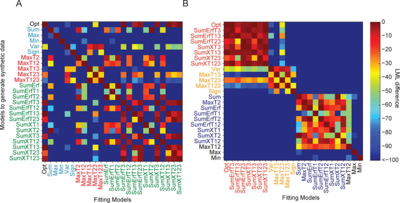
We tested how well synthetic data sets generated from each model (rows) were fitted by each model (columns). (A) Model confusion matrix. The color in a cell represents the difference in log marginal likelihood between a model and the winning model for the corresponding data set. Dark red on the diagonal means that the model used to generate the data was found to be most likely. (B) As in (A), but with models clustered by Agreement. Models in red are models with high Agreement to the Opt model. Models in blue are from a different model set with low Agreement to the Opt model, but similar to each other. Models in orange have higher Agreement to the Opt than to the blues models, but they are still well distinguishable from the Opt model. Also refer to Fig. 8C.

Figure A2. Model comparison based on information criteria.

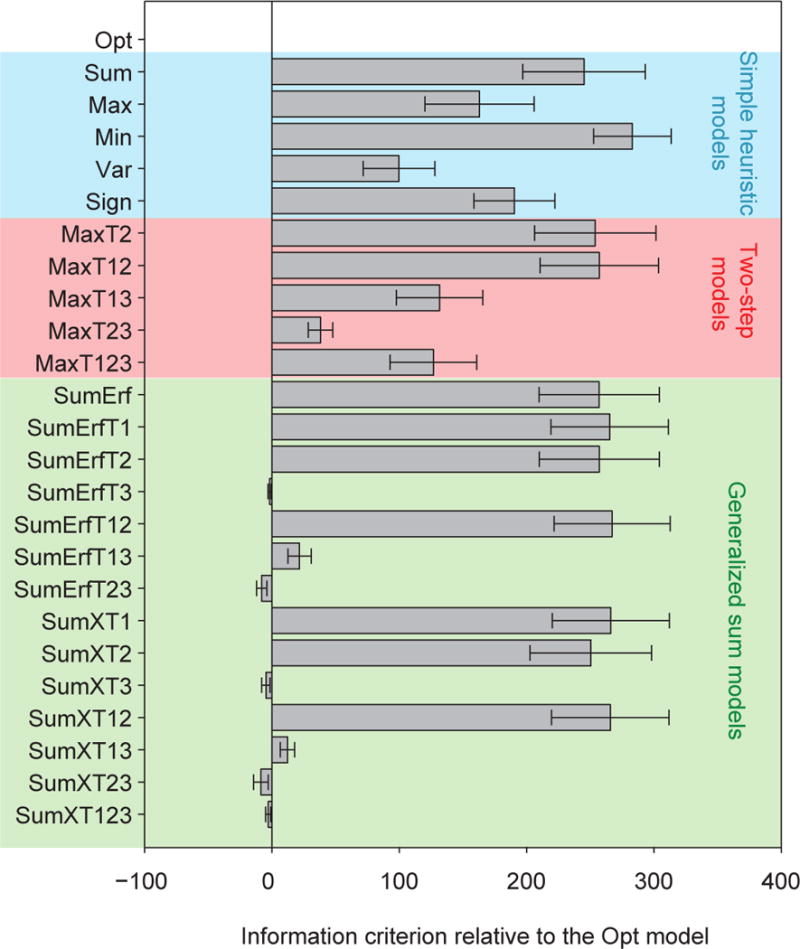
Mean and s.e.m. across subjects of the difference in information criterion (AICc or BIC) between each model and the Opt model. Note that all models have two parameters, therefore all information criteria yield the same differences between models.

Figure A3. Correlation between log marginal likelihood and Agreement with any one model given the real data.

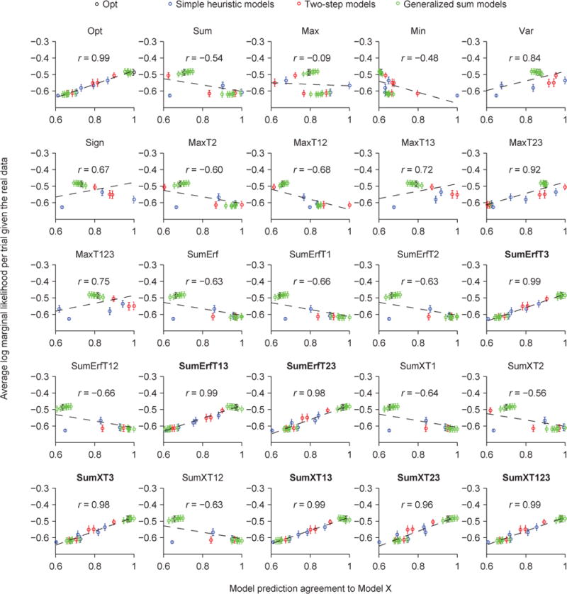
Related to Fig. 8D and Fig. 9A. Each plot shows, given the real data, the mean (open circle) and s.e.m. (error bar) across subjects of a model’s average log marginal likelihood per trial as a function of its Agreement with a reference model; the reference model differs between plots. The dashed line represents the best linear fit. r is the Pearson correlation. The names of eight best models are in boldface.

Figure A4. Correlation between log marginal likelihood and Agreement with the Opt model given synthetic data generated from any one model.

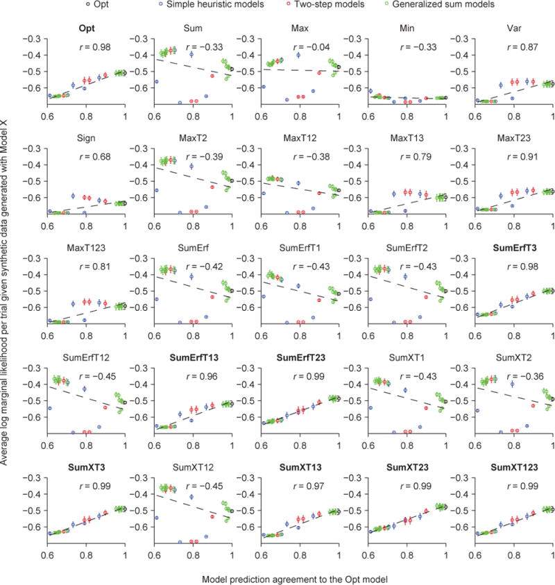
Related to Fig. 9B. For each plot, we generated 9 synthetic data sets from a different generating model. The plot shows the mean (open circle) and s.e.m. (error bar) of a model’s average log marginal likelihood per trial as a function of its Agreement with the Opt model based on those data sets. The dashed line represents the best linear fit. r is the Pearson correlation. The names of eight best models are in boldface. Given synthetic data generated from one of the eight best models, the correlation is high. Given synthetic data generated from a model outside of the eight best, the correlation is low.

Figure A5. Correlation between log marginal likelihood and Agreement with a reference model given synthetic data generated from that reference model.

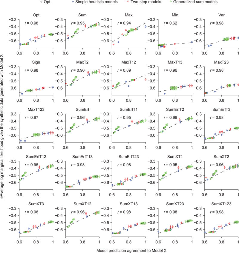
Related to Fig. 9C. For each plot, we generated 9 synthetic data sets from a different generating model. The plot shows the mean (open circle) and s.e.m. (error bar) of a model’s average log marginal likelihood per trial as a function of its Agreement with the generating model. The dashed line represents the best linear fit. r is the Pearson correlation. Given synthetic data generated from any one model, the correlation is high.

References

- Acuna DE, Berniker M, Fernandes HL, Kording KP. Using psychophysics to ask if the brain samples or maximizes. Journal of Vision. 2015;15:1–16. doi: 10.1167/15.3.7. [DOI] [PMC free article] [PubMed] [Google Scholar]
- Alais D, Burr D. Ventriloquist Effect Results from Near-Optimal Bimodal Integration. Current Biology. 2004;14(3):257–262. doi: 10.1016/j.cub.2004.01.029. [DOI] [PubMed] [Google Scholar]
- Ashby FG, Maddox WT. Human category learning. Annual Review of Psychology. 2005;56:149–178. doi: 10.1146/annurev.psych.56.091103.070217. [DOI] [PubMed] [Google Scholar]
- Baldassi S, Burr DC. Feature-based integration of orientation signals in visual search. Vision Research. 2000;40:1293–1300. doi: 10.1016/s0042-6989(00)00029-8. [DOI] [PubMed] [Google Scholar]
- Baldassi S, Verghese P. Comparing integration rules in visual search. Journal of Vision. 2002;2:559–570. doi: 10.1167/2.8.3. [DOI] [PubMed] [Google Scholar]
- Battaglia PW, Hamrick JB, Tenenbaum JB. Simulation as an engine of physical scene understanding. Proceedings of the National Academy of Sciences of the United States of America. 2013;110(45):18327–32. doi: 10.1073/pnas.1306572110. [DOI] [PMC free article] [PubMed] [Google Scholar]
- Borg I, Groenen PJF. Modern Multidimensional Scaling. Vol. 94 Springer; 2005. Series in Statistics. [Google Scholar]
- Bowers JS, Davis CJ. Bayesian just-so stories in psychology and neuroscience. Psychological Bulletin. 2012;138(3):389–414. doi: 10.1037/a0026450. [DOI] [PubMed] [Google Scholar]
- Chater N. Reconciling simplicity and likelihood principles in perceptual organization. Psychological Review. 1996;103(3):566–581. doi: 10.1037/0033-295X.103.3.566. [DOI] [PubMed] [Google Scholar]
- Chater N, Tenenbaum JB, Yuille A. Probabilistic models of cognition: conceptual foundations. Trends in Cognitive Sciences. 2006;10(7):287–91. doi: 10.1016/j.tics.2006.05.007. [DOI] [PubMed] [Google Scholar]
- Chen SY, Ross BH, Murphy GL. Implicit and explicit processes in category-based induction: is induction best when we don’t think? Journal of Experimental Psychology General. 2014;143(1):227–46. doi: 10.1037/a0032064. [DOI] [PubMed] [Google Scholar]
- Coenen A, Rehder B, Gureckis T. Decisions to intervene on causal systems are adaptively selected. Cognitive Science. 2014:343–348. doi: 10.1016/j.cogpsych.2015.02.004. [DOI] [PubMed] [Google Scholar]
- Collett D. Modelling Binary Data, Second Edition. CRC Press; 2002. [Google Scholar]
- Cover TM, Thomas JA. Elements of Information Theory. Elements of Information Theory 2005 [Google Scholar]
- Deneve S. Bayesian spiking neurons II: learning. Neural Computation. 2008;20(1):118–145. doi: 10.1162/neco.2008.20.1.118. [DOI] [PubMed] [Google Scholar]
- Dienes PZ, McLeod P. Do fielders know where to go to catch the ball, or only how to get there? 1996;22(3):531–543. [Google Scholar]
- Eckstein MP. The lower visual search efficiency for conjunctions is due to noise and not serial attentional processing. Psychological Science. 1998;9:111–118. [Google Scholar]
- Ernst MO, Banks MS. Humans integrate visual and haptic information in a statistically optimal fashion. Nature. 2002;415(6870):429–433. doi: 10.1038/415429a. [DOI] [PubMed] [Google Scholar]
- Faisal AA, Wolpert DM. Near optimal combination of sensory and motor uncertainty in time during a naturalistic perception-action task. Journal of Neurophysiology. 2009;101(4):1901–12. doi: 10.1152/jn.90974.2008. [DOI] [PMC free article] [PubMed] [Google Scholar]
- Fiser J, Berkes P, Orbán G, Lengyel M. Statistically optimal perception and learning: from behavior to neural representations. Trends in Cognitive Sciences. 2010;14:119–130. doi: 10.1016/j.tics.2010.01.003. [DOI] [PMC free article] [PubMed] [Google Scholar]
- Fleming SM, Maloney LT, Daw ND. The irrationality of categorical perception. The Journal of Neuroscience : The Official Journal of the Society for Neuroscience. 2013;33(49):19060–70. doi: 10.1523/JNEUROSCI.1263-13.2013. [DOI] [PMC free article] [PubMed] [Google Scholar]
- Geisler WS. Contributions of ideal observer theory to vision research. Vision Research. 2011;51(7):771–81. doi: 10.1016/j.visres.2010.09.027. [DOI] [PMC free article] [PubMed] [Google Scholar]
- Geisler WS, Perry JS. Contour statistics in natural images. Visual Neuroscience. 2009;26(1):109–121. doi: 10.1017/S0952523808080875. [DOI] [PMC free article] [PubMed] [Google Scholar]
- Gigerenzer G. Striking a Blow for Sanity in Theories of Rationality. Models of a Man: Essays in Memory of Herbert A Simon. 2004:389–409. [Google Scholar]
- Gigerenzer G, Gaissmaier W. Heuristic decision making. Annual Review of Psychology. 2011;62:451–82. doi: 10.1146/annurev-psych-120709-145346. [DOI] [PubMed] [Google Scholar]
- Gigerenzer G, Goldstein DG. Reasoning the fast and frugal way: models of bounded rationality. Psychological Review. 1996;103(4):650–669. doi: 10.1037/0033-295x.103.4.650. [DOI] [PubMed] [Google Scholar]
- Grassberger P. Finite sample corrections to entropy and dimension estimates. Physics Letters A. 1988;128(6–7):369–373. [Google Scholar]
- Grassberger P. Entropy Estimates from Insufficient Samplings. arXiv, 5. Data Analysis, Statistics and Probability; Computational Physics 2003 [Google Scholar]
- Green DM, Swets JA. Society. Vol. 1. Peninsula Pub; 1966. Signal detection theory and psychophysics. [Google Scholar]
- Griffiths TL, Chater N, Kemp C, Perfors A, Tenenbaum JB. Probabilistic models of cognition: exploring representations and inductive biases. Trends in Cognitive Sciences. 2010;14(8):357–364. doi: 10.1016/j.tics.2010.05.004. [DOI] [PubMed] [Google Scholar]
- Griffiths TL, Tenenbaum JB. Optimal predictions in everyday cognition. Psychological Science. 2006;17(9):767–773. doi: 10.1111/j.1467-9280.2006.01780.x. [DOI] [PubMed] [Google Scholar]
- Gu Y, Angelaki DE, Deangelis GC. Neural correlates of multisensory cue integration in macaque MSTd. Nature Neuroscience. 2008;11(10):1201–1210. doi: 10.1038/nn.2191. [DOI] [PMC free article] [PubMed] [Google Scholar]
- Hamming RW. Error Detecting and Error Correcting Codes. Bell System Technical Journal. 1950;29(2):147–160. [Google Scholar]
- Hopfield JJ, Tank DW. “Neural” computation of decisions in optimization problems. Biological Cybernetics. 1985;52:141–152. doi: 10.1007/BF00339943. [DOI] [PubMed] [Google Scholar]
- Hornik K, Stinchcombe M, White H. Multilayer feedforward networks are universal approximators. Neural Networks. 1989;2(5):359–366. [Google Scholar]
- Jazayeri M, Movshon JA. A new perceptual illusion reveals mechanisms of sensory decoding. Nature. 2007;446(7138):912–5. doi: 10.1038/nature05739. [DOI] [PMC free article] [PubMed] [Google Scholar]
- Jones M, Love BC. Bayesian Fundamentalism or Enlightenment? On the explanatory status and theoretical contributions of Bayesian models of cognition. The Behavioral and Brain Sciences. 2011;34(4):169–88. doi: 10.1017/S0140525X10003134. disuccsion 188–231. [DOI] [PubMed] [Google Scholar]
- Körding KP, Beierholm U, Ma WJ, Quartz S, Tenenbaum JB, Shams L. Causal inference in multisensory perception. PloS One. 2007;2(9):e943. doi: 10.1371/journal.pone.0000943. [DOI] [PMC free article] [PubMed] [Google Scholar]
- Körding KP, Wolpert DM. The loss function of sensorimotor learning. Proceedings of the National Academy of Sciences of the United States of America. 2004;101(26):9839–9842. doi: 10.1073/pnas.0308394101. [DOI] [PMC free article] [PubMed] [Google Scholar]
- Kramer P, Graham N, Yager D. Simultaneous measurement of spatial-frequency summation and uncertainty effects. Journal of the Optical Society of America A, Optics and Image Science. 1985;2(9):1533–1542. doi: 10.1364/josaa.2.001533. [DOI] [PubMed] [Google Scholar]
- Landy MS, Goutcher R, Trommershäuser J, Mamassian P. Visual estimation under risk. Journal of Vision. 2007;7(6):4. doi: 10.1167/7.6.4. [DOI] [PMC free article] [PubMed] [Google Scholar]
- López-Moliner J, Field DT, Wann JP. Interceptive timing: prior knowledge matters. Journal of Vision. 2007;7(13):11.1–8. doi: 10.1167/7.13.11. [DOI] [PubMed] [Google Scholar]
- Ma WJ. Signal detection theory, uncertainty, and Poisson-like population codes. Vision Research. 2010;50(22):2308–19. doi: 10.1016/j.visres.2010.08.035. [DOI] [PubMed] [Google Scholar]
- Ma WJ. Organizing probabilistic models of perception. Trends in Cognitive Sciences. 2012;16(10):511–518. doi: 10.1016/j.tics.2012.08.010. [DOI] [PubMed] [Google Scholar]
- Ma WJ, Jazayeri M. Neural Coding of Uncertainty and Probability. Annual Review of Neuroscience. 2014;37:205–220. doi: 10.1146/annurev-neuro-071013-014017. [DOI] [PubMed] [Google Scholar]
- Ma WJ, Navalpakkam V, Beck JM, van Den Berg R, Pouget A. Behavior and neural basis of near-optimal visual search. Nature Neuroscience. 2011;14(6):783–790. doi: 10.1038/nn.2814. [DOI] [PMC free article] [PubMed] [Google Scholar]
- Ma WJ, Shen S, Dziugaite G, van den Berg R. Requiem for the max rule? Vision Research. 2015 doi: 10.1016/j.visres.2014.12.019. [DOI] [PMC free article] [PubMed] [Google Scholar]
- Maloney LT, Mamassian P. Bayesian decision theory as a model of human visual perception: testing Bayesian transfer. Visual Neuroscience. 2009;26(1):147–155. doi: 10.1017/S0952523808080905. [DOI] [PubMed] [Google Scholar]
- Maloney LT, Trommershäuser J, Landy MS. Questions without words: A comparison between decision making under risk and movement planning under risk. Integrated models of cognitive systems. 2007:297–314. [Google Scholar]
- Mazyar H, Van den Berg R, Seilheimer RL. Independence is elusive : Set size effects on encoding precision in visual search. Journal of Vision. 2013;13(5):1–14. doi: 10.1167/13.5.8. [DOI] [PMC free article] [PubMed] [Google Scholar]
- McLeod P, Reed N, Dienes Z. Psychophysics: how fielders arrive in time to catch the ball. Nature. 2003;426:244–245. doi: 10.1038/426244a. [DOI] [PubMed] [Google Scholar]
- Morales J, Solovey G, Maniscalco B, Rahnev D, de Lange FP, Lau H. Low attention impairs optimal incorporation of prior knowledge in perceptual decisions. Attention, Perception, & Psychophysics. 2015:2021–2036. doi: 10.3758/s13414-015-0897-2. [DOI] [PubMed] [Google Scholar]
- Nessler B, Pfeiffer M, Buesing L, Maass W. Bayesian Computation Emerges in Generic Cortical Microcircuits through Spike-Timing-Dependent Plasticity. PLoS Computational Biology. 2013;9(4) doi: 10.1371/journal.pcbi.1003037. [DOI] [PMC free article] [PubMed] [Google Scholar]
- Nessler B, Pfeiffer M, Maass W. Hebbian Learning of Bayes Optimal Decisions. Advances in Neural Information Processing Systems. 2008:1169–1176. [Google Scholar]
- Nolte LW, Jaarsma D. More on the Detection of One of M Orthogonal Signals. The Journal of the Acoustical Society of America. 1967 Aug;41:497. [Google Scholar]
- Norris D. The Bayesian reader: Explaining word recognition as an optimal Bayesian decision process. Psychological Review. 2006;113(2):327–357. doi: 10.1037/0033-295X.113.2.327. [DOI] [PubMed] [Google Scholar]
- Osherson DN, Smith EE, Wilkie O, López A, Shafir E. Category-based induction. Psychological Review. 1990;97(2):185–200. [Google Scholar]
- Palmer J, Verghese P, Pavel M. The psychophysics of visual search. Vision Research. 2000;40:1227–1268. doi: 10.1016/s0042-6989(99)00244-8. [DOI] [PubMed] [Google Scholar]
- Pouget A, Beck JM, Ma WJ, Latham PE. Probabilistic brains: knowns and unknowns. Nature Neuroscience. 2013;16(9):1170–8. doi: 10.1038/nn.3495. [DOI] [PMC free article] [PubMed] [Google Scholar]
- Qamar AT, Cotton RJ, George RG, Beck JM, Prezhdo E, Laudano, Tolias AS, Ma WJ. Trial-to-trial, uncertainty-based adjustment of decision boundaries in visual categorization. Proceedings of the National Academy of Sciences of the United States of America. 2013;110(50):20332–20337. doi: 10.1073/pnas.1219756110. [DOI] [PMC free article] [PubMed] [Google Scholar]
- Rauber HJ, Treue S. Reference repulsion when judging the direction of visual motion. Perception. 1998;27:393–402. doi: 10.1068/p270393. [DOI] [PubMed] [Google Scholar]
- Seydell A, McCann BC, Trommershäuser J, Knill DC. Learning stochastic reward distributions in a speeded pointing task. The Journal of Neuroscience : The Official Journal of the Society for Neuroscience. 2008;28(17):4356–4367. doi: 10.1523/JNEUROSCI.0647-08.2008. [DOI] [PMC free article] [PubMed] [Google Scholar]
- Simon HA. Rational choice and the structure of the environment. Psychological Review. 1956;63:129–138. doi: 10.1037/h0042769. [DOI] [PubMed] [Google Scholar]
- Spiegelhalter DJ, Best NG, Carlin BP, Van Der Linde A. Bayesian measures of model complexity and fit. Journal of the Royal Statistical Society Series B: Statistical Methodology. 2002;64:583–616. [Google Scholar]
- Steyvers M, Tenenbaum JB, Wagenmakers EJ, Blum B. Inferring causal networks from observations and interventions. Cognitive Science. 2003;27 [Google Scholar]
- Szpiro SFa, Spering M, Carrasco M. Perceptual learning modifies untrained pursuit eye movements. Journal of Vision. 2014;14(8):1–13. doi: 10.1167/14.8.8. [DOI] [PMC free article] [PubMed] [Google Scholar]
- Trommershauser J, Körding KP, Landy MS. Sensory Cue Integration. Computational Neuroscience. Oxford University Press; 2011. [Google Scholar]
- Wason PC. On the failure to eliminate hypotheses in a conceptual task. Quarterly Journal of Experimental Psychology. 1960;12(3):129–140. [Google Scholar]
- Wei XX, Stocker AA. A Bayesian observer model constrained by efficient coding can explain “anti-Bayesian” percepts. Nature Neuroscience. 2015;18(10):1509–17. doi: 10.1038/nn.4105. [DOI] [PubMed] [Google Scholar]
- Wichmann Fa, Hill NJ. The psychometric function: I. Fitting, sampling, and goodness of fit. Perception & Psychophysics. 2001;63(8):1293–1313. doi: 10.3758/bf03194544. [DOI] [PubMed] [Google Scholar]
- Wozny DR, Beierholm UR, Shams L. Probability matching as a computational strategy used in perception. PLoS Computational Biology. 2010;6(8) doi: 10.1371/journal.pcbi.1000871. [DOI] [PMC free article] [PubMed] [Google Scholar]