Capturing Heterogeneous Group Differences using Mixture-of-Experts : Application to a Study of Aging

Abstract

In MRI studies, linear multi-variate methods are often employed to identify regions or connections that are affected due to disease or normal aging. Such linear models inherently assume that there is a single, homogeneous abnormality pattern that is present in all affected individuals. While kernel-based methods can implicitly model a non-linear effect, and therefore the heterogeneity in the affected group, extracting and interpreting information about affected regions is difficult. In this paper, we present a method that explicitly models and captures heterogeneous patterns of change in the affected group relative to a reference group of controls. For this purpose, we use the Mixture-Of-Experts (MOE) framework, which combines unsupervised modeling of mixtures of distributions with supervised learning of classifiers. MOE approximates the non-linear boundary between the two groups with a piecewise linear boundary, thus allowing discovery of multiple patterns of group differences. In the case of patient/control comparisons, each such pattern aims to capture a different dimension of a disease, and hence to identify patient subgroups. We validated our model using multiple simulation scenarios and performance measures. We applied this method to resting state functional MRI data from the Baltimore Longitudinal Study of Aging, to investigate heterogeneous effects of aging on brain function in cognitively normal older adults (> 85 years) relative to a reference group of normal young to middle-aged adults (< 60 years). We found strong evidence for the presence of two subgroups of older adults, with similar age distributions in each subgroup, but different connectivity patterns associated with aging. While both older subgroups showed reduced functional connectivity in the Default Mode Network (DMN), increases in functional connectivity within the pre-frontal cortex as well as the bilateral insula were observed only for one of the two subgroups. Interestingly, the subgroup showing this increased connectivity (unlike the other subgroup) was, cognitively similar at baseline to the young and middle-aged subjects in two of seven cognitive domains, and had a faster rate of cognitive decline in one of seven domains. These results suggest that older individuals whose baseline cognitive performance is comparable to that of younger individuals recruit their “cognitive reserve” later in life, to compensate for reduced connectivity in other brain regions.

Graphical abstract

1. Introduction

A growing number of projects (Shock et al., 1984; Satterthwaite et al., 2014; Van Essen et al., 2012; Biswal et al., 2010) and consortia (Di Martino et al., 2014) are collecting MR-based neuroimaging data from a large number of individuals to investigate the complex patterns of brain change associated with non-pathological and pathological processes, such as effects of development, aging, injury or disease. While MRI has been successfully used to understand functional and structural disruptions, in many studies, the main objective is to compare two groups of subjects, i.e. between normal controls and patients, or younger and older, with the assumption that the specific condition affects all subjects in a uniform, homogeneous fashion. In other words, each affected subject is assumed to possess the same pattern of abnormality. This approach conflicts with what is observed in clinical assessments, which point to inherently multi-dimensional symptoms or cognitive changes (Ylikoski et al., 1999) that reflect a broad “spectrum” of changes associated with disease or developmental and maturational processes. Machine learning tools provide a great opportunity for investigating the heterogeneity of patterns of brain change associated with various diseases and processes, which have been for the most part ignored in previous studies.

In this paper, we extend the analytical framework of two-group comparisons, where a diseased or otherwise affected group is compared to a relatively more normal reference group. We propose the application of a method that combines unsupervised clustering and supervised learning of classifiers to identify heterogeneity of brain changes in the affected group. Our main assumption is that the affected group was subjected to a heterogeneous underlying pathological or non-pathological process. Thus, the affected group consists of multiple subgroups, each of which has a different pattern of group differences, relative to the reference group. We assume that normal variation in the brain in the reference group evolves into potentially multiple patterns of abnormality or differences in the affected group, which are presumably caused by a variety of underlying potential pathological processes. As illustrated in Figure 1, in the space of multi-dimensional MRI data, the affected group “deviates” from the reference group along many different directions. We are interested in (1) capturing these heterogeneous patterns of group differences and, (2) identifying subgroups within the affected group that are associated with each pattern of group difference.

Figure 1.

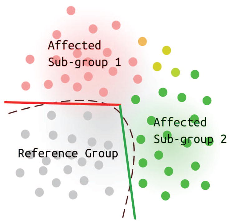
An illustration that shows heterogeneity in the discriminating boundary, relative to a reference group. Non-linear classifiers can implicitly model non-linearity but estimating the boundary (dashed lines) in high dimensional spaces is difficult. The proposed Mixture-of-Experts can approximate the non-linear curve with a piece-wise linear boundary (red and green lines) and find subgroups associated with each line (red and green points).

It may be possible to identify heterogeneity in the affected group by applying a purely unsupervised clustering method to the affected group alone. However, in medical imaging data, two-group differences are often small and subtle, and can be nearly orthogonal to the dominant direction of variance. Running a purely unsupervised clustering method produces clusters along this direction, which may not be relevant to the problem we are attempting to solve - to find heterogeneity in the discriminating boundary that reflects the underlying pathologic process. Hence our attempt to solve this problem involves using the reference group as an “anchor”. In other words, we assume that the reference group is transformed by an underlying process which affects the reference group in multiple different ways. We would like to identify these multiple directions of deviation from the reference group. In our proposed method, allowing the reference group to be equally shared amongst all subgroups is an indirect manner of modeling this deviation from the reference group.

We propose the use of a Mixture-of-Experts (MOE) framework (Jacobs et al., 1991) to capture heterogeneous patterns of brain change. The MOE framework was initially proposed for vowel discrimination within speech recognition (Jacobs et al., 1991) and later, as a fast and efficient alternative to “kernel” SVMs (Ladicky and Torr, 2011; Fu et al., 2010). The MOE method combines unsupervised clustering with supervised classification to approximate the non-linear boundary that separates the two classes with a piece-wise linear separating boundary. Thus, it provides us the identification of the subgroups as well as the multivariate patterns that discriminate each subgroup from the reference group. The data is modeled using a mixture of distributions, by assigning a soft subgroup membership to each subject in the affected group. The linear boundary between each affected subgroup and the reference group can be found using a linear classifier, such as a linear Support Vector Machine (linear-SVM). We describe the MOE method in detail in the methods section. We thoroughly validate the MOE method using multiple simulation cases and four validation measures used to quantify its performance; these results follow the methods section.

While kernel SVMs can also successfully model non-linear separation boundaries between groups, such as the one shown in Figure 1, they suffer from a major limitation in neuroimaging applications, namely the lack of interpretability of the results. In a kernel-based method, the data is implicitly projected into a higher dimensional space prior to being classified and the non-linear separating boundary in the original feature space is not explicitly computed. This limitation was tackled in multiple papers (Golland, 2001; Fan et al., 2007; Rasmussen et al., 2011). Golland (2001) find reflections of each support vector of the fitted kernel-SVM on the other side of the separating boundary. The difference between the support vector and its reflection is the local discriminant direction in the feature space, which is interpreted in terms of the changes to the input data. Similarly, in COMPARE (Fan et al., 2007), Fan et. al average these local discriminant directions across all support vectors, resulting in a single group difference map. In Rasmussen et al. (2011), the importance of each feature for the classifier is estimated by computing the average extent to which predictions get perturbed when the data points are perturbed. This results in a single sensitivity map for the non-linear classifier. However, none of these approaches targeted the identification of subgroups in the population based on the discriminant direction of change in comparison to the reference group. An easily interpretable and not overly complex way of representing this heterogeneity is necessary for the clinical adoption of such methods.

There are a few prior studies that aimed to capture heterogeneity using machine learning tools. For example, in Song et al. (2010), the authors first propose clustering the subjects within each group, followed by supervised learning. In Sabuncu et al. (2009), the authors propose a joint clustering-coregistration algorithm, which can compute data-driven templates that summarize the different modes in the population. However, as discussed earlier, a purely unsupervised method may be insufficient to identify heterogeneous disease patterns. In Filipovych et al. (2011, 2012), the author proposed the use of a maximum margin based approach to identify latent group memberships. More recently, (Varol et al., 2015) proposed the use of a maximum margin polytope method to identify variations in disease using T1-structural data. While the methods proposed by Filipovych et al. (2011); Varol et al. (2015) bear resemblance to the proposed MOE method, there are significant methodological differences. The proposed MOE approach is a well-understood, well-established approach which combines an expert (classifier/regressor) with a mixture model (clustering), and hence falls under the umbrella of generative-discriminative methods. On the other hand, both the formulations of Filipovych et al. (2011); Varol et al. (2015) contain only maximal margin classification objectives, and are hence purely discriminative; they rely on the distance to the hyperplane to determine the grouping of the subjects. This difference is crucial, as the MOE not only models the distance from the hyperplane but also the natural clustering that may be present within the affected group, for identification of heterogeneity. As we will describe in the methods section later, this difference is also reflected in the prediction of new test cases. In the polytope method, a new test sample is classified as a patient if the sample falls outside the polytope (i.e., it uses the signed distance from each of the sides of the polytope to determine if the point is inside, or outside). On the other hand, the MOE model first evaluates the distance from the test sample to each of the cluster centroids, then performs classification.

The MOE method is applied to real MRI data for identification of heterogeneous patterns of brain change due to aging, a very important and challenging problem in neuroimaging. Increased life expectancy and booming population growth has resulted in an ever growing proportion of older people across the globe. This has led to a greater prevalence of age-related cognitive impairment, including Alzheimers disease, which, in addition to the social cost, also places a huge burden on institutionalized health care resources. Aging is accompanied by highly heterogeneous processes that change brain structure and function in multiple ways. Understanding and quantifying such changes and their associations with age-related cognitive decline and impairment is critical for development of imaging bio-markers that flag early disease stages or deviations from normal aging trajectories.

Our approach is applied to data from the Baltimore Longitudinal Study on Aging (BLSA) (Shock et al., 1984). BLSA is a long running study of physical and psychological aging that includes comprehensive cognitive assessments and brain MR imaging measurements for a large sample of well-characterized volunteer participants. Of these, resting state fMRI (rsfMRI), acquired since 2010, has emerged as a useful tool in the arsenal of imaging bio-markers. However, functional brain changes can be highly heterogeneous across individuals, in part due to different underlying pathologic processes and in part due to heterogeneity in functional response across individuals. This challenge highlights the need for using analytical tools that can capture such heterogeneity. In this paper, we used the MOE method to capture heterogeneous patterns of age-related differences in a group of older individuals (> 85 years, n = 41) relative to a reference group of younger individuals (< 60 years, n = 46). We identify subgroups among the older subjects such that each subgroup shows a different pattern of abnormal functional connectivity. (Note that in this work, we use “affected” to refer to deviations from a reference group though we do not know whether these deviations reflect pathological or maturational processes.) In addition, based on the results obtained from MOE, we examine the resulting subgroups with respect to longitudinal changes in cognitive function relative to the younger group.

In the following section we describe the MOE formulation, the optimization strategy and the model validation steps. The validation of the performance of the method using simulated data is described in Section 3. Section 4 describes the heterogeneous effects of aging on functional connectivity found using BLSA data. We discuss the advantages and limitations of our method, and the importance of our findings in Section 5 and summarize our conclusions in Section 6.

2. Mixture-of-Experts: Formulation, Optimization and Testing

Consider a binary classification problem with data x_i ∈ R^D obtained from i = 1, 2, . . .N subjects. Each subject is associated with a binary label y_i ∈ {−1, 1}, −1 for the reference group and +1 for the affected group. We assume that the discriminative direction is not constant across the feature space. In other words, the group difference is heterogeneous due to multiple processes that might affect brain structure and function in different ways. This heterogeneity can be modeled using multiple piece-wise linear hyperplanes. Our objective is to learn the multiple discriminant patterns of abnormality along with subgroups of affected subjects corresponding to each pattern. We propose to model this heterogeneity with a piece-wise linear boundary with K segments. Each segment is a hyperplane w^k, which is interpretable in terms of the discriminative/affected features in each subgroup k.

2.1. The expert model

Let ${\mathbf{m}}_i=[m_i^1,m_i^2,\dots ,m_i^K]$, m_i ∈ [0, 1], ${\sum }_{k=1}^K{m}_i^k=1$ indicate the relative membership of subject i to group k. Recall that along the discriminative direction, subjects deviate in multiple different directions due to underlying process, away from the reference group. Therefore we associate the reference subjects with all K hyperplanes, i.e., if y_i = −1, $m_i^k=1/K\forall k$. If the membership values were known for all subjects, the k^th linear-SVM hyperplane w^k ∈ R^D can be learned by solving the following optimization problem (Bishop et al., 2006):

$$\underset{{\mathbf{w}}^k}{\text{minimize}}\frac{1}{2}{\Vert {\mathbf{w}}^k\Vert }_1+C\sum _{i=1}^N{m}_i^k{(1-y_i{({\mathbf{w}}^k)}^T{\mathbf{x}}_i)}_{+}^2$$ (1)

where $x_{+}^2=max(0,x^2)$ is the ℓ₂-positive norm.

The above optimization problem is the standard formulation of the ℓ₁-regularized ℓ₂-loss SVM in its primal form, with the membership values $m_i^k$ acting as sample weights. The user-defined SVM cost parameter C controls the extent to which misclassified points are penalized. Note that the intercept of the SVM hyperplane has been subsumed into the variable w^k by appending a constant value to all data points. For more details about the SVM formulation, please see SI Section 3.

2.2. The mixture model

The unknown group membership values m_i can be obtained by jointly optimizing the SVM objective function (above) with a data clustering objective. In this paper, we learn these subgroups using Fuzzy-C-Means (Bezdek et al., 1984). Each one of K subgroups is associated with a centroid d^k. The mixture model is formulated as an optimization problem, as follows:

$$\begin{array}{l}\underset{{\left\{{\mathbf{d}}^k\right\}}_k,{\left\{m_i^k\right\}}_{i,k}}{\text{minimize}}\sum _{k=1}^K\sum _{i=1}^N{(m_i^k)}^a{\Vert {\mathbf{x}}_i-{\mathbf{d}}^k\Vert }_F^2\\ \text{subject}\text{to}\sum _{k=1}^K{m}_i^k=1,m_i^k\in [0,1]n=1,\dots ,N\end{array}$$ (2)

As explained in (Bezdek et al., 1984), the “fuzzyness ” coefficient m controls the “softness” of the membership assignments. When m = 1, the memberships are hard (binary). As m → ∞, the membership values tend to 1/K, where K is the number of sub-groups.

In our model, we set the “fuzziness” coefficient a to a value of 2. We make this choice because when the cluster centroids (and other variables) are known, for a = 2, the minimization problem becomes a quadratic programming problem, which is convex. Therefore, if the values of all other variables are known, convergence to the global optimum is guaranteed.

2.3. The joint model

Bringing the optimization problems 1 and 2 together, we get

$$\begin{array}{l}\underset{{\left\{{\mathbf{w}}^k\right\}}_k,{\left\{m_i^k\right\}}_{i,k}}{\text{minimize}}\sum _{k=1}^K\left\{\frac{1}{2}{\Vert {\mathbf{w}}^k\Vert }_1+C\sum _{i=1}^N{m}_i^k{(1-y_i{({\mathbf{w}}^k)}^T{\mathbf{x}}_i)}_{+}^2+\lambda \sum _{i=1}^N{(m_i^k)}^a{\Vert {\mathbf{x}}_i-{\mathbf{d}}^k\Vert }_F^2\right\}\\ \text{subject}\text{to}\sum _{k=1}^K{m}_i^k=1,m_i^k\in [0,1]n=1,\dots ,N\end{array}$$ (3)

where λ is a user-defined value that controls the trade-off between the cost of classification and clustering. The other user-defined parameters are the number of groups K, and the SVM cost-value C.

2.4. Optimization strategy

We use alternating minimization to solve for the cluster centroids d^k, membership values $m_i^k$ and the SVM hyperplanes w^k. Note that, from the joint optimization problem in Eq. 3, only the membership values $m_i^k$ are common to both the classification and the clustering problems. Knowing these values would allow us to decompose the joint optimization problem into K + 1 smaller problems, which are all convex: K weighted-SVM objectives with weighted samples, and solving for cluster centroids. We use lib-linear with weighted samples (Fan et al., 2008) to solve each of the K SVM objectives, and the cluster centroids can be updated as follows:

$${\mathbf{d}}^k=\frac{{\sum }_{i=1}^N{(m_i^k)}^a{\mathbf{x}}_i}{{\sum }_{i=1}^N{(m_i^k)}^a}$$ (4)

When the values of variables w^k and d^k are known, the joint problem can be decomposed into N optimization problems, one for each subject. Each of these N problem can be solved for the membership values $m_i^1,m_i^2,\dots ,m_i^K$ of subject i, as follows:

$$\begin{array}{l}\underset{{\left\{m_i^k\right\}}_k}{\text{minimize}}\sum _{k=1}^K\left\{C{e}_i^k{m}_i^k+\lambda {\Vert {\mathbf{x}}_i-{\mathbf{d}}^k\Vert }_F^2{(m_i^k)}^a\right\}\\ \text{subject}\text{to}\sum _{k=1}^K{m}_i^k=1,m_i^k\in [0,1]\end{array}$$ (5)

When a = 2, the objective function is quadratic and convex, and the constraints are linear.

The optimization strategy alternately solves for d^k, $m_i^k$ and w^k until convergence. Convexity of each of the sub-problems guarantees its convergence to a local minimum.

2.5. Testing the MOE model

We use ten-fold cross-validation to evaluate the fit of the model to the data. Given a test subject x* with an unknown label y*, first the unknown membership values m* are obtained by solving the clustering objective alone with x* as the data. Then the label y* is determined as the sign of the weighted combination of individual SVM predictions as follows:

$$y^{\ast }=\text{sign}\left(\sum _{k=1}^K{m}_k^{\ast }\text{sign}({({\mathbf{w}}^k)}^T{\mathbf{x}}^{\ast })\right)$$ (6)

We use four summary measures to quantify the performance of the method:

1. Cross-validated accuracy: Estimated labels are compared with the known labels of the left out fold. This testing is repeated for all folds for multiple runs to obtain an averaged cross-validation accuracy.

2. Maximum pair-wise inner product: For K > 1, we compute the maximum normalized inner product between all pairs of hyperplanes, as follows:

   $$r_{\mathbf{w}}=max\left\{\frac{{({\mathbf{w}}^k)}^T{\mathbf{w}}^l}{{\Vert {\mathbf{w}}^k\Vert }_2{\Vert {\mathbf{w}}^l\Vert }_2},\forall k,l\in \{1,2,\dots ,K\}\right\}$$ (7)

   This value measures the extent to which the hyperplanes have rotated away from each other.

3. Cluster Reproducibility: For K > 1, we evaluate the reproducibility of the subgroups across repeated runs of the proposed method. We use the Adjusted-Rand Index (ARI) for fuzzy cluster assignments, as defined in Brouwer (2009). The ARI is a scalar value between [−1, 1] which measures the extent to which two fuzzy cluster assignments are similar, after adjusting for chance. An ARI value of +1 denotes perfect reproducibility, 0 indicates that some subjects have the same fuzzy membership solely due to chance and −1 indicates disagreement among all pairs of memberships. See SI Section 4 for mathematical details.

4. Cluster Separation Index: For K > 1, we evaluate the extent to which the K clusters are separated across repeated runs of the proposed method. We use the Bezdek Partition Coefficient (BPC) (Bezdek, 1981; Dave, 1996) which provides a scalar value between [0, 1] for each fuzzy clustering assignment. A value of 1 indicates full cluster separation, i.e., cluster assignments for all subjects are binary. A value of 0 indicates no separation, i.e., cluster assignments for all subjects are equal to 1/K, where K is the number of clusters. See SI Section 4 for mathematical details.

2.6. Selecting user-defined parameters

The user-defined parameters of the MOE method are the number of subgroups K, the SVM cost value C and the classification-clustering trade-off parameter λ. We use a grid-based search to find those parameters for which the four above mentioned measures (accuracy, maximum inner-product, cluster reproducibility, cluster separation) are optimal. As we will show later using simulated as well as real data, we found that changing the number of subgroups K, resulted in the largest change in the four measures. Therefore, for fixed C = λ = 1, we vary K = 1, 2, 3, . . . in order to find the optimal value of K. Once this value is found, we repeat the grid-search for C and λ jointly.

3. Experiments with Simulated Data

3.1. Simulated Data

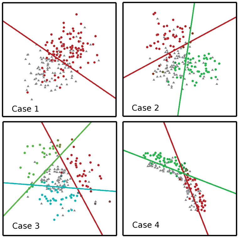
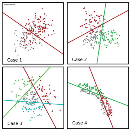
We evaluated the capacity of the proposed method in revealing underlying subgroups using four two-dimensional simulated datasets. These datasets reflected different heterogeneity patterns in the affected subgroups, defined as the subgroups deviating from the reference group:

• Case 1: One affected subgroup with a single pattern of change relative to a reference group. Each group is modeled by an isotropic Gaussian distribution.

• Case 2: Two affected subgroups, with heterogeneous patterns of change relative to a reference group. Each subgroup is modeled by an isotropic Gaussian distribution.

• Case 3: Multiple affected subgroups, with heterogeneous patterns of change relative to a reference group. This is modeled using concentric circles

• Case 4: Multiple affected subgroups, with heterogeneous patterns of change relative to a reference group. This is modeled using arcs of concentric circles For each case, 200 points were simulated, with 100 affected and 100 reference subjects. In each of the four cases above, 20% of the data points were deliberately mis-classified.

3.2. MOE choice of parameters and results

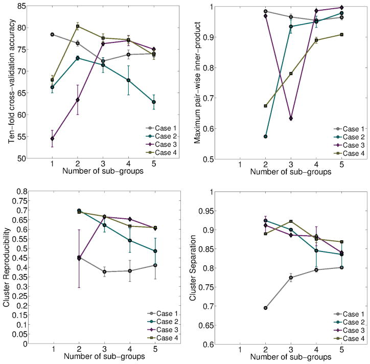
We measured (1) ten-fold cross-validation accuracy (2) maximum normalized inner-product between the resulting $\left(\begin{array}{c}K\\ 2\end{array}\right)$ pairs of hyperplanes (3) reproducibility of the resulting affected subgroups, measured using ARI and (4) separation of the resulting affected subgroups, measured using BPC. These results are shown in Figures 3 and 4. We expect a good model to provide high cross-validated accuracy, low inner-product (large angle between hyperplanes), high reproducibility of the resulting subgroups across runs, and high separability between subgroups.

Figure 3.

Variation in four cross-validated performance measures for K = {1, 2, . . . , 5}, for each of the four simulated cases. From top-left, clockwise: Accuracy, Maximum inner-product, cluster separation and cluster reproducibility. Results from each case is plotted in a different color.

Figure 4.

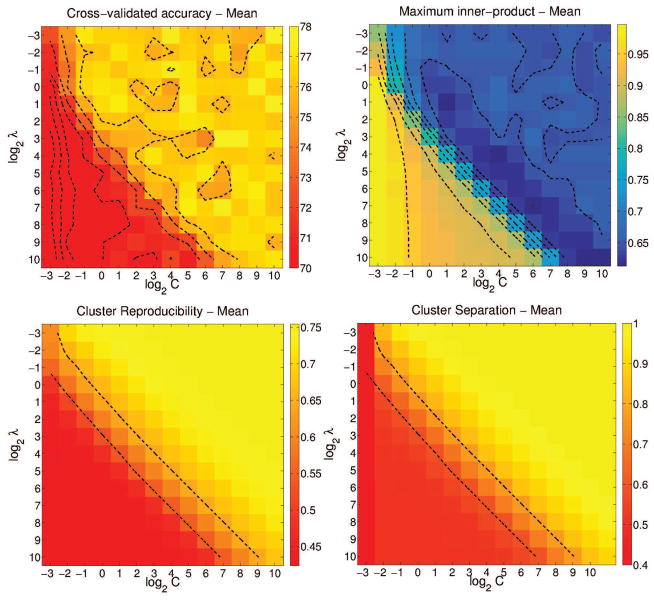
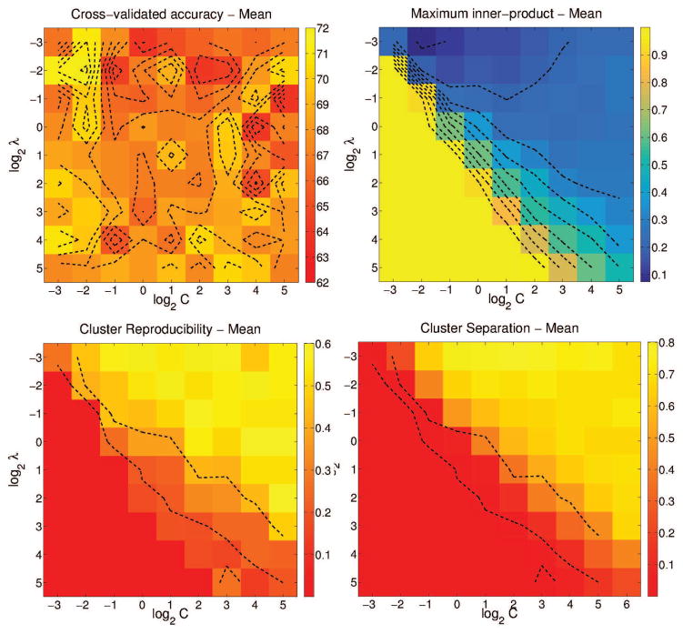
Variation in four cross-validated performance measures for K = 3, C, λ = {2⁻³, 2⁻², . . . , 2¹⁰}, for Case 3. From top-left, clockwise: Accuracy, Maximum inner-product, cluster separation and cluster reproducibility.

From Figure 3, we observe that highest accuracy values are obtained for K values of 2, 3, and 2 for the cases 2, 3, and 4 respectively. For the same three values, the inner-product between the hyper-planes is at a minimum, suggesting that the hyperplanes have rotated to their maximum extent. Cluster reproducibility and separation are also high. Note that in the absence of heterogeneity, as simulated in Case 1, the fuzziness of the clustering algorithm prevents the creation of spurious noise-based clusters; the membership value of each affected subject will be close to 1/K and consequently, the resulting hyperplanes are almost identical, and cluster separation is low, as seen in Case 1.

For Case 3, and for K = 3, we used a grid-based search to evaluate the three measures for C = {2⁻³, 2⁻², . . . , 2¹⁰} and λ = {2⁻³, 2⁻², . . . , 2¹⁰}. In all four plots, the parameter space is clearly split into two: C ≥ λ – 3 and C < λ – 3. When C ≥ λ – 3, the inner-product measure is low and the accuracy, cluster reproducibility and separation indices are high. Considering all these observations together, the values K = 2, C = 2¹⁰ and λ = 2⁻³ seem reasonable, with ten-fold cross-validation accuracy at 78±0.8%, normalized inner-product at 0.5 ± 0.01, ARI at 0.75 ± 0.08 and BPC at 1. Animations showing the convergence of the MOE method for the simulation cases is shown in SI Section 6.

Table 1 shows the ten-fold cross-validation accuracy of MOE model compared with that of an RBF-kernel SVM for each of the four simulated cases. In Cases 2–4, the accuracy of the MOE model is slightly lower than the nonlinear model. This difference in accuracy is highest for Case 3, where the non-linearity is the greatest among all four cases. This decrease is expected, as a piece-wise linear model is used to approximate the non-linearity. The MOE model performed with a small drop in accuracy, when compared to nonlinear models, while providing interpretable results and explicit assignment into a small number of subgroups. Such interpretability is very important for adoption of such methods in clinical environments.

Table 1.

Table comparing ten-fold cross-validation accuracy for MOE method vs. Gaussian-kernel SVM, for four simulated cases.

Simulation Case	1	2	3	4
Gaussian-kernel SVM	79.0 ± 0.54	75.4 ± 1.08	86 ± 0.01	85.3 ± 0.27
MOE	79.0 ± 0.22	74.1 ± 0.74	77.9 ± 0.80	82.5 ± 1.35

3.3. Effect of adding noisy dimensions

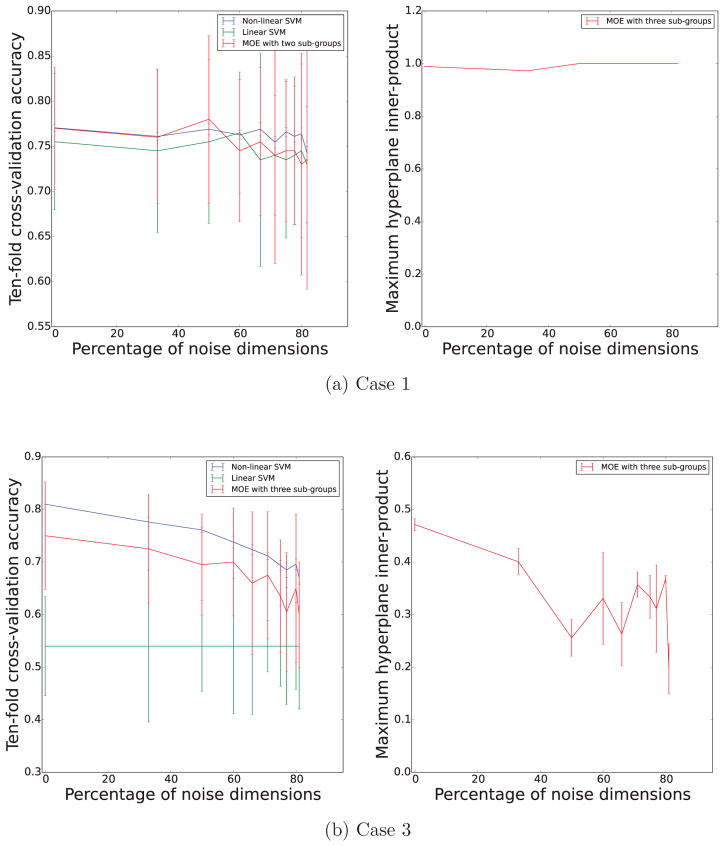
The higher performance of the MOE compared to the linear SVM is a clear indication of the presence of heterogeneity. However, note that the MOE method does not provide a better accuracy when compared to the nonlinear SVM classifier. Even with high-dimensional settings, the piece-wise linear MOE classifier can only approximate a non-linear boundary, therefore can only perform as well as the non-linear classifier, and no more. In order to test this, we ran experiments with increasing amount of noisy dimensions to simulated data (case 3). We evaluated the cross-validated accuracy and maximum hyper-plane inner-product as the the number of noisy dimensions increased. The results are shown in Figure 5. It is clear that the accuracy of the MOE is firmly in between the linear-SVM and the non-linear SVM. This makes sense, as the complexity of the MOE is in between the two methods.

Figure 5.

Plot showing variation in cross-validated accuracy and maximum inner-product values as the number of noisy dimensions is increased.

From these experiments we observed that, for Case 1, when there is no underlying heterogeneity in the data, the accuracy and inner-product values stay almost constant when the number of noisy dimensions are increased. For the non-linear Case 3, as the number of noisy dimensions are increased, accuracy for both the non-linear SVM as well as the MOE drop, and the hyperplanes become increasingly dissimilar. At 100% noise, the accuracy drops to chance (AUC=0.5) and inner-product drops to 0.

For real rsfMRI data, the true dissimilarity value and the number of noisy dimensions is data and modeling specific; the rate at which these values change is dependent on the separation between the groups, constraints imposed by the model and the value of the free parameters (cost and trade-off value). However, for a fixed dataset, the inner-product value is comparable across different parameter choices. In Fig 5, as the number of sub-groups is increased, the inner-product value shows a clear and consistent increase, suggesting that the dissimilarity is highest when K = 2.

4. Capturing heterogeneity in aging using BLSA data

4.1. Data

Demographics

We used data acquired as a part of the Baltimore Longitudinal Study of Aging. We considered around 50 participants at both age extremes. In addition we restricted our sample only to those individuals with low head motion during the acquisition, measured using Mean Relative Displacement - MRD < 0.25mm (Satterthwaite et al., 2012). Further, we excluded subjects who met criteria for onset of Mild Cognitive Impairment or Alzheimer’s disease at time of scan. The final sample we used has 41 older subjects in the age range 83 – 96 years and 46 younger subjects aged 27 – 60 years.

rsfMRI Data

Images were acquired at the NIA clinical research facility on a Philips Achieva 3T MRI scanner, with an in plane resolution of 3 × 3mm, slice thickness of 4 mm, TR/TE=2000/30s and total scan duration of 6 minutes. We used a validated confound regression procedure (Satterthwaite et al., 2012) with non-linear DRAMMS registration (Ou et al., 2011). We used GRaSP (Honnorat et al., 2015), which is a data-driven method used for parcellating the grey matter based on local functional connectivity of the voxels. GRaSP provided a common group parcellation with 596 spatially localized parcels (See SI Section 2 for an image of the parcellation). Using this parcellation, we computed connectivity matrices of size 596 × 596 using Pearson’s correlation coefficient for each subject.

We used sparsity-based dimensionality reduction using a recently published Sparse Learning (SL) approach (Eavani et al., 2015), in order to reduce the high-dimensionality of the correlation data (≈ 178000 connections). SL is a data-driven method that generates multiple whole-brain sparse connectivity patterns (SCPs) that characterize functional connectivity in a group of subjects. Each SCP consists of regions whose average connectivity co-varies across subjects. It also generates scalar measures (SCP coefficients) reflecting the average connectivity within respective SCPs in each individual subject. Unlike seed-based correlation, the SL method is not dependent on a priori knowledge of a seed region, but rather extracts dominant connectivity patterns in an unbiased manner. SCPs are neither orthogonal, nor independent and allow for spatial overlap and anti-correlations among regions. Thus they greatly aid interpretability and visualization of the results, compared to conventional correlation matrix data. Correlation matrices are input as-is to the method which does not require the removal of low and negative correlation values. The SL approach can be applied to the data in a hierarchical manner - each “primary” SCP can be further divided into smaller “secondary” SCPs by reapplying the method to only those regions assigned to the primary SCP. See SI Section 1 for details of the method.

This method requires two user-defined parameters to be specified - the number of SCPs and the sparsity level of SCPs, at each level of the hierarchy. We considered two levels in the hierarchy - primary and secondary. In the primary level, using cross validation to evaluate reproducibility and data fit of the SCPs, we estimated 10 SCPs at a sparsity level of 30% of gray matter coverage. In the secondary level, each SCP was split further into 10 more SCPs, each at a sparsity level of 30% of the primary SCP coverage. In this manner, we obtain 10 primary + 100 secondary SCPs, along with 110 total SCP coefficients for each subject.

Controlling for motion confound

Head motion during acquisition of rsfMRI scans is known to affect functional connectivity in a systematic manner (Power et al., 2012). This is problematic in studies of aging as older subjects generally move more, making motion a nuisance confounder (Mowinckel et al., 2012). In this study, in order to mitigate the effects of motion, we incorporated three corrective steps in various stages of the pre-processing pipeline. First, we restricted our analysis to only those subjects with a summary motion (MRD) value of less than 0.25mm. Second, the global signal was regressed out of the voxel-wise data, as it is known to be a good surrogate measure for the effect of motion and other physiological effects on BOLD signal (Satterthwaite et al., 2012). Performing GSR pre-processing also better delineates SCPs (For SCPs generated without GSR, pleae see SI Section 7). Finally, after the SCPs are computed, the MRD values were regressed out of each SCP’s coefficients at the group-level. These motion-corrected coefficients are used as input to the MOE method.

Cognitive Assessments

BLSA participants receive a battery of cognitive tests at every visit. Participants are assessed in seven cognitive domains, listed below:

1. California Verbal Learning Task (CVLT) was used to assess verbal learning and memory. Higher values indicate better performance.

2. Benton Visual Retention Test (BVRT) quantifies figural memory and visuo-constructional ability. Lower values indicate better performance.

3. CARD Rotation Test (CRT) measure the ability to mentally manipulate figures. Higher values indicate better performance.

4. Letter Fluency (FLULET) measures phonemic fluency. Higher values indicate better performance.

5. Category Fluency (FLUCAT) measures semantic fluency. Higher values indicate better performance.

6. Trail Making Test Part A (TRATS) was used as an indicator of visual attention and processing speed. Lower values indicate better performance.

7. Trail Making Test Part B (TRBTS) was used to evaluate executive function. Lower values indicate better performance.

As BLSA is an ongoing longitudinal study, we have cognitive data from multiple cognitive assessments for each participant over up to a 19 year period prior to, and concurrent with, the time of scan. However, participants have varying numbers of visits and cognitive assessments. Therefore, every participant’s cognitive performance in each of the seven domains is summarized using three measurements. For each of the 3 * 7 = 21 measurements, we evaluate whether the subgroups obtained using the MOE model (using the SCP data alone) showed differences. These analyses are listed below:

• Cross-sectional analysis: We examine cross-sectional effects using cognitive data that was collected concurrent with the rsfMRI scans. This provides us with seven concurrent measurements for each participant. We performed one-way analysis of variance (ANOVA) for each of these seven measurements.

• Longitudinal analysis of cognitive rate of change (slope): As we mentioned earlier, many participants made multiple visits over a 19 year period; using these multiple time-points, we computed the cognitive rate of change for each domain. This provides seven slope measurements for each participant. We use linear mixed models to test whether the slope values are equal across the subgroups.

• Longitudinal analysis of baseline cognitive value (baseline): We also compared the cognitive performance of each participant from their first visit to the BLSA. This provides seven measurements of “baseline” cognitive values for each participant. As before, we use linear mixed models to test whether the baseline values are equal across the subgroups.

4.2. Choice of MOE Parameters K, C and λ for BLSA data

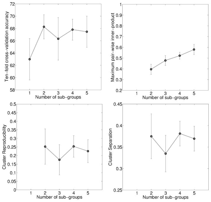
As before, we first evaluated the performance of the method with the parameters λ = C = 1 and the number of experts K was varied between one and five. Figure 6 shows the ten-fold cross-validation accuracy, maximum inner-product, cluster reproducibility and cluster separability plotted as a function of K. It is easily seen that the accuracy increases to 69% for K = 2 and beyond. The inner-product plot also shows the maximum divergence of the hyperplanes at K = 2.

Figure 6.

Variation in four cross-validated performance measures for K = {1, 2, . . . , 5}, for BLSA data. From top-left, clockwise: Accuracy, Maximum inner-product, cluster separation and cluster reproducibility.

With K fixed at 2, we varied the value of the parameters C, λ = {2⁻³, 2⁻², . . . , 2⁵}. The behavior of the MOE method with actual rsfMRI data is similar to that in simulated data (Figures 3, 4). The cross-validated accuracy plot does not show any clear trend. In the other three plots, when C ≥ 0.75(λ – 1), the inner-product measure is lower and the cluster reproducibility and separation indices are higher. Considering all these observations together, a good choice of parameter values is K = 2, C = 2⁻² and λ = 2⁻³, with ten-fold cross-validation accuracy at 70±0.8%, normalized inner-product at 0.15 ± 0.01, ARI at 0.51 ± 0.06 and BPC at 0.44 ± 0.02. Compared to this, the ten-fold cross-validation accuracy for RBF-kernel SVM on the same data is 72.39 ± 1.47%, with optimal RBF-kernel parameters C = 2¹, γ = 2⁻⁵.

4.3. MOE results : Subgroups and discriminant hyper-planes Subgroups identified by MOE model

We binarized the soft membership values provided by the MOE model by assigning each older individual to the cluster with higher membership value. We will call the resulting two older subgroups SG1 and SG2. This yielded 25 participants in SG1, 16 participants in SG2. With these hard assignments, we used a standard linear SVM to classify SG1 from SG2. The resulting ten-fold cross-validated accuracy for SG1 vs. SG2 is 84.87 ± 2.05%.

MOE Hyper-planes w¹,w²

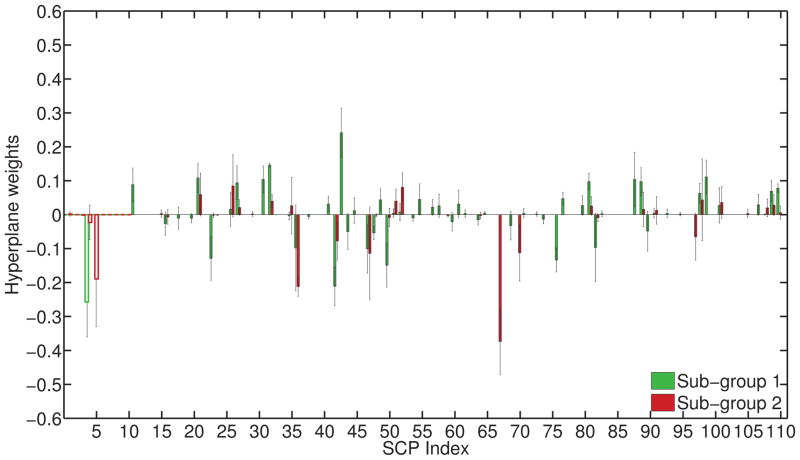
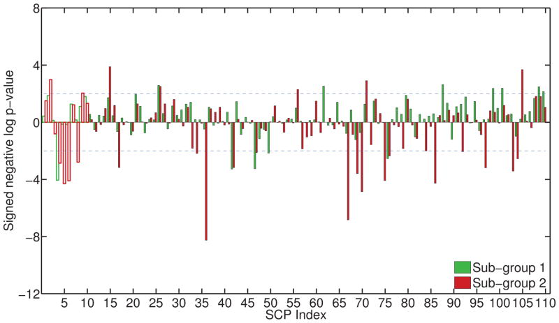
For K = 2, C = 0.25, λ = 0.125, weights of the separating hyperplanes for the two subgroups are plotted in Fig. 8. The hyperplanes are clearly different from each other, as indicated by separability of the two groups (accuracy for SG1 vs. SG2: 84.87%, inner-product b/w hyperplanes: 0.15). Using the binarized assignments, we compared SCP coefficients of the two older subgroups with the younger group using uni-variate t-tests. The resulting p-values are shown in Figure 9. The y-axis plots the negative logarithm of the p-value, multiplied by the sign of the t-value (reflecting the direction of change). On observing the results in Fig. 9, we notice both similarities and differences in the manner in which aging affects both sub-groups. In general, both subgroups show somewhat similar trends of aging related effects; however, SG2 shows significantly higher connectivity in many SCPs, while SG1 does not.

Figure 8.

Hyperplane weights w¹,w², with variation across runs also plotted. A positive hyperplane weight indicates that the corresponding SCP coefficient is reduced in older subjects. SG1 (green) mainly shows connectivity decreases, and a few increases. SG2 (red) predominantly shows connectivity increases. The weights for primary SCPs are shown as an outline.

Figure 9.

Plot showing the result of uni-variate comparison of SCP coefficients between younger subjects and the two older subject groups. The y-axis measures the signed negative log p-value: −log₁₀(p) * sign(t), where t: t-statistic and p: p-value. Decreased connectivity results in a positive value, increased connectivity in a negative value. Comparison of young vs. SG1 is shown in green, young vs. SG2 is shown in red. The p-values for primary SCPs are shown as an outline.

Differences in terms of SCPs

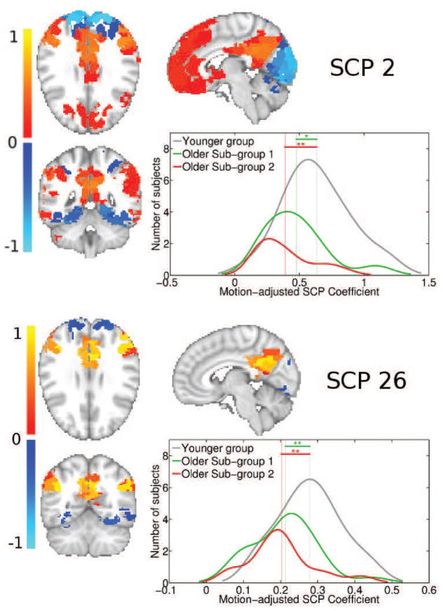
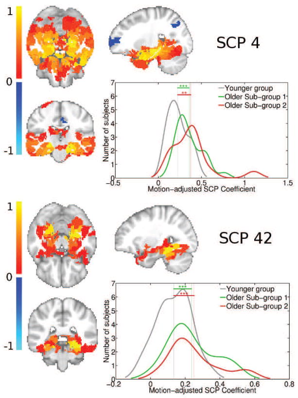
SCPs whose associated coefficients showed high significant differences between young and SG1, and young and SG2 are plotted in Figures 10,11,12 and 13. For each of the primary SCPs, the secondary SCP with the highest significant difference is also shown. As seen in Figure 10, SCP 2 and 26 captures the Default Mode (DM) regions and its anti-correlation with the medial visual regions. The average connection strength between the precuneus and bilateral inferior parietal regions are significantly reduced in both older subgroups.

Figure 10.

Plot showing primary SCP 2, and its associated secondary SCP 26, whose average connectivity is reduced in both older subgroups. SCP 2 shows the Default Mode (DM) regions (red-yellow) and their anti-correlation with the medial visual areas (blue-light blue). SCP 26 captures the posterior regions of SCP 2 - the precuneus and the inferior parietal regions. The distribution fit of the underlying SCP coefficient histograms are also shown, for each SCP and for each subgroup. Significance levels is indicates as follows: ’***’ for p-value < 0.001, ’**’ for p-value < 0.01 and ’*’ for p-value < 0.05.

Figure 11.

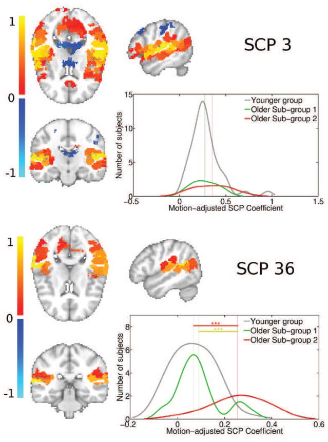
Plot showing primary SCP 3, and its associated secondary SCP 36, whose average connectivity is increased in the second older subgroup, but not the first. SCP 3 highlights most of the bilateral insula. SCP 36 captures the posterior bilateral insula and supramarginal gyrus. The distribution fit of the underlying SCP coefficient histograms are also shown, for each SCP and for each subgroup. Significance levels is indicates as follows: ’***’ for p-value < 0.001, ’**’ for p-value < 0.01 and ’*’ for p-value < 0.05.

Figure 12.

Plot showing primary SCP 4, and its associated secondary SCP 42, whose average connectivity is increased in both older subgroups. SCP 4 delineates most of the temporal lobe. SCP 42 highlights the bilateral para-hippocampal gyri and temporal fusiform cortex. The distribution fit of the underlying SCP coefficient histograms are also shown, for each SCP and for each subgroup. Significance levels is indicates as follows: ’***’ for p-value < 0.001, ’**’ for p-value < 0.01 and ’*’ for p-value < 0.05.

Figure 13.

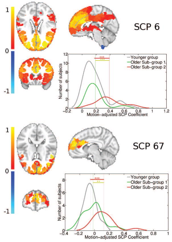
Plot showing primary SCP 6, and its associated secondary SCP 67, whose average connectivity is increased in the second older subgroup, but not the first. SCP 2 highlights most of the pre-frontal cortex. SCP 67 captures the bilateral para-cingulate gyrus and inferior temporal gyrus. The distribution fit of the underlying SCP coefficient histograms are also shown, for each SCP and for each subgroup. Significance levels is indicates as follows: ’***’ for p-value < 0.001, ’**’ for p-value < 0.01 and ’*’ for p-value < 0.05.

Figure 11 shows SCPs 3 and 36, which capture the Sylvian fissure and insula. As SCP 36 shows, the average bilateral connectivity in the bilateral posterior insula and supramarginal gyrus is increased in older SG2 relative the younger group, but not in SG1.

Figure 12 shows SCPs 4 and 42, which delineate areas in the temporal lobe, specifically the bilateral hippocampal and parahippocampal regions. The average connectivity between the bilateral temporal regions is increased in both older subgroups compared to the younger group.

Figure 13 shows primary SCP 6 and associated secondary SCP 67. Both SCPs indicate that the bilateral connectivity between regions within the prefrontal cortex is significantly increased in SG2, but not SG1, relative to the younger group.

Demographic and cognitive differences between subgroups

The older subgroups did not differ significantly in terms of age or sex. Using linear mixed-models, we found that SG2 significantly differed from SG1 in the TRBTS score at time-of-scan (p-value 0.051). In addition, using ANOVA and pair-wise tests, we found that SG2 significantly differed from SG1 in the baseline value of trail-making tests A and B (TRATS and TRBTS), with p-values 0.0078 and < 0.0001 respectively. For both measures, SG2 performed as well as the younger participants, whereas SG1 performed at a significantly lower level. However, analysis of cognitive rates of decline (slope) revealed that for the BVRT test of visual retention, SG2 declined at a significantly faster rate than SG1 (p-value 0.0501). These results are summarized in Tables 2, 3 and 4. Results of all statistical tests for both the concurrent and longitudinal analyses are summarized in SI tables 1, 2 and 3.

Table 2.

Cross-sectional analysis: Table listing significant ANOVA results from cross-sectional analysis of concurrent cognitive scores obtained at time-of scan. The number of subjects for which this data was available, and the mean and standard error estimates for each group are also provided.

Test	Number of subjects	Mean estimate (Std. Error)			p-value	Pair-wise p-value
		Younger subjects	SG1	SG2		Younger vs SG1	Younger vs SG2	SG1 vs SG2
TRBTS	60	57.8(4.9)	110.8(8.5)	84.4(10.2)	< 0.0001	< 0.0001	0.022	0.051

Table 3.

Longitudinal analysis: Table listing significant ANOVA results from analysis of baseline of longitudinal cognitive trajectories. The number of assessments for which this data was available, and the mean and standard error estimates for each group are also provided.

Test	Number of subjects (assessments)	Mean baseline estimate (Std. Error) p-value				Pair-wise p-value
		Younger subjects	SG1	SG2		Younger vs SG1	Younger vs SG2	SG1 vs SG2
TRATS	81(336)	28.0(1.9)	40.1(2.3)	30.4(2.9)	0.0003	< 0.0001	0.48	0.0078
TRBTS	82(336)	60.7(5.4)	105.8(6.6)	62.0(8.5)	< 0.0001	< 0.0001	0.90	< 0.0001

Table 4.

Longitudinal Analysis: Table listing significant ANOVA results from analysis of slope of longitudinal cognitive trajectories. The number of assessments for which this data was available, and the mean and standard error estimates for each group are also provided.

Test	Number of subjects (assessments)	Mean slope estimate (Std. Error)			p-value	Pair-wise p-value
		Younger subjects	SG1	SG2		Younger vs SG1	Younger vs SG2	SG1 vs SG2
BVRT	86(345)	0.058(0.073)	0.099(0.073)	0.32(0.082)	0.049	0.69	0.020	0.0501

Motion differences between sub-groups

Mean MRD values for each sub-group are summarized in Table 5. Results of two-group t-tests comparing MRD values are summarized in Table 6. As expected, older participants move significantly more than the younger participants. However, there is no significant difference in the mean MRD value between the two older sub-groups.

Table 5.

Mean Relative Displacement summarized for each group

Younger subjects	Older subjects	SG1	SG2
0.11 ± 0.04	0.13 ± 0.04	0.12 ± 0.04	0.13 ± 0.05

Table 6.

p-values obtained using two-group t-tests comparing MRD values

Younger vs. Older	Younger vs. SG1	Younger vs. SG2	SG1 vs. SG2
0.03	0.13	0.03	0.44

5. Discussion

In this paper, we proposed the use of a Mixture-of-Experts framework to capture diverse disease or degeneration patterns. This is a general framework that can be applied to any type of data (structural or functional MR data) using any expert (classification or regression-based) and any mixture model (K-Means, fully Gaussian mixtures and others). We used a linear-SVM along with fuzzy c-means clustering to identify multiple subgroups in the heterogeneous population, along with the associated abnormal connectivity pattern for each subgroup. We evaluated the resulting models based on four factors - cross-validated accuracy, maximum hyperplane inner-product, cluster reproducibility and cluster separation.

We tested the performance of the method using multiple 2-D simulation cases. As we stated earlier, multiple linear SVMs are used to approximate the non-linear boundary between the two groups, hence there is some loss of accuracy. This loss in accuracy is traded for a richer description of the data in terms of multiple subgroups and linear hyperplanes associated with each subgroup, that are interpretable in terms of changes to the underlying features. Furthermore, as fuzzy membership values are used, in the absence of heterogeneity in the data, the fuzziness of the model prevents the generation of noisy clusters.

We applied this method to rsfMRI data from the BLSA in order to determine whether heterogeneous patterns of functional connectivity changes occur in the aging brain, relative to younger adults. We found strong evidence for the presence of two older subgroups SG1 and SG2, with a classification accuracy of 84% between them. These subgroups were identified in a completely data driven manner solely from the rsfMRI data, without using any additional demographic or cognitive information. The results show both similarities and differences in the manner in which SCPs were affected in the two older subgroups, SG1 and SG2. While the trend (direction) of differences for the two sub-groups was similar, SG2 showed highly significant increases for certain SCPs, while SG1 did not. Using scores obtained from a battery of cognitive tests, further investigation revealed that SG1 generally had lower cognitive scores at baseline. However, in tests measuring attention and executive function, SG2 performed as well as the younger subjects, while SG1 performed poorly, at baseline and at time-of-scan.

Both older subgroups show decreased connectivity between posterior regions of the default mode network (SCP 26), consistent with other reports in literature linking reduced DM connectivity and aging (Damoiseaux et al., 2008; Andrews-Hanna et al., 2007). In addition, there is evidence that posterior DM regions are vulnerable to early amyloid deposition, which occurs many years before the appearance of cognitive impairment associated with AD (Buckner et al., 2005). These factors could contribute to the connectivity differences observed between the younger and older groups.

The older subgroups also show increased connectivity between the bilateral occipital-fusiform and para-hippocampal regions, which are associated with episodic memory. A recent study supports this finding (Salami et al., 2014). In addition, there is some evidence for increased activation in the MTL in MCI as well (Kircher et al., 2007; Dickerson et al., 2004).

The two older subgroups also show divergent patterns of functional connectivity, relative to younger subjects. SG2 demonstrated increased bilateral connectivity in the pre-frontal areas (SCP 6, 70), whereas SG1 did not. Increased frontal connectivity has been widely reported in other studies of age effects on connectivity (Buckner, 2004; Reuter-Lorenz and Cappell, 2008; Tisserand and Jolles, 2003). The Posterior-Anterior Shift in Aging (PASA) model (Davis et al., 2008) hypothesizes that increased frontal activity compensates for the age-related reduction in activity in posterior regions. These results suggest that a similar posterior to anterior shift in functional connectivity may also occur in some older individuals with increasing age. SG2 also had significantly increased connectivity in the bilateral posterior insular cortex and supramarginal gyrus (Heinzel et al., 2013). This increase was not seen in SG1. The results of the MOE model inform us that not all older subjects show the same patterns of increased and reduced connectivity. Indeed, only older subjects who performed as well as the younger subjects in specific cognitive tests (TRATS and TRBTS) at baseline, and declined faster in others (BVRT), displayed this compensatory effect, while older subjects with lower performance at baseline did not functionally compensate.

In this paper, we have shown several advantages of applying the MOE model to identify heterogeneity using both simulated and real data. However a methodological limitation to consider is that as the MOE model combines classification with a clustering objective, it inherits the drawbacks of clustering as well. High dimensional data, such as voxel wise three-dimensional images is difficult to cluster due to the well known “curse of dimensionality” (Steinbach et al., 2004). The effectiveness of applying our method for voxel-level analysis needs to be investigated further. The Sparse Learning method used in this paper provides an interpretable connectivity-based set of SCP bases, while reducing data dimension, making it applicable for MOE analysis.

Another limitation to consider is the trade-off between higher accuracy and better interpretability. The MOE classifier can only approximate a nonlinear boundary. Therefore, in terms of accuracy, it can only perform as well as the non-linear classifier, and no more. In fact, in both simulated and real rsfMRI data, the MOE classifier slightly under performs the nonlinear classifier. Our motivation behind proposing the MOE classifier as an alternative is for the sake of interpretability, to discover heterogeneous two-group differences.

Our method primarily looks for variation in discriminating direction, and may not directly relate to disease/aging severity. Individuals that are further away from the hyperplane have greater magnitude of changes relative to the reference group, therefore has a more severe disease/aging effect. Thus severity can be estimated by calculating the distance of each subject from the discriminating hyperplane. Such an approach has been been used in prior studies to quantify severity of the disorder, such as Alzhiemers’ and Mild Cognitive Impairment (Davatzikos et al., 2009; Clark et al., 2012) and Autism Spectrum Disorder (Ingalhalikar et al., 2011). Currently, MOE provides information about heterogeneity alone. In addition to the sub-group memberships, severity along each heterogenous aging direction is also potentially very useful; this will be investigated in the future.

A possible extension of this method is to incorporate heterogeneity in the reference group as well, considering that the variability in a typical reference “normal” group can be quite high. Using such an extension, each estimated affected group is associated with its closest set of reference subjects. This is advantageous, as the associated hyperplane weights and associated two-group p-values are more specific to the disease/aging heterogeneity. On the other hand, the hyperplanes are no longer comparable across sub-groups, as the reference group is different for each affected sub-group. The advantages and trade-offs of such an extension need to be investigated further.

6. Conclusion

The proposed Mixture-of-Experts method approximates a non-linear classification boundary with multiple linear hyperplanes. In this manner, it allows identification of sub-groups of individuals in the affected group, each with a different pattern of variation relative to the reference group. Our framework is generic, and it can capture heterogeneous effects in any type of data. The performance of the method was tested and validated on simulated data using multiple performance metrics, which evaluate the behavior of the method. Applied to rsfMRI data from BLSA, we found strong evidence for two subgroups of older individuals. The participants in the first subgroup had lower cognition at baseline, and they showed significant reductions in DM connectivity relative to younger subjects. The participants in the second subgroup were cognitively similar to the younger group at baseline in two of seven cognitive domains, and they showed compensatory increases in pre-frontal cortex, bilateral insula and supramarginal gyri, in addition to decreased DM connectivity. These results demonstrate that our method is a valuable analysis tool that can capture heterogeneity in manifestation of disease or age-related brain changes.

Figure 2.

Four simulated cases used to evaluate the performance of the method. The hyper-planes and subgroups obtained using MOE are also shown using a different color for each hyper-plane and associated subgroup.

Figure 7.

Variation in four cross-validated performance measures for K = 2, C, λ = {2⁻³, 2⁻², . . . , 2⁵}, for BLSA data. From top-left, clockwise: Accuracy, Maximum inner-product, cluster separation and cluster reproducibility.

Highlights.

• Mixture of Experts model for heterogeneity identification

• Approximates a non-linear classification boundary with piece-wise linear boundary

• Identifies multiple affected sub-groups based on variation of the decision boundary

• Using BLSA resting state connectivity data, two distinct older sub-groups were found

• Older sub-group that was cognitively similar to younger at baseline had higher conn. in insula, frontal lobes

References

- Andrews-Hanna JR, Snyder AZ, Vincent JL, Lustig C, Head D, Raichle ME, Buckner RL. Disruption of large-scale brain systems in advanced aging. Neuron. 2007;56(5):924–935. doi: 10.1016/j.neuron.2007.10.038. [DOI] [PMC free article] [PubMed] [Google Scholar]
- Bezdek JC. Pattern recognition with fuzzy objective function algorithms. Kluwer Academic Publishers; 1981. [Google Scholar]
- Bezdek JC, Ehrlich R, Full W. Fcm: The fuzzy c-means clustering algorithm. Computers & Geosciences. 1984;10(2):191–203. [Google Scholar]
- Bishop C, et al. Pattern recognition and machine learning. Vol. 4. Springer; New York: 2006. [Google Scholar]
- Biswal BB, Mennes M, Zuo XN, Gohel S, Kelly C, Smith SM, Beckmann CF, Adelstein JS, Buckner RL, Colcombe S, et al. Toward discovery science of human brain function. Proceedings of the National Academy of Sciences. 2010;107(10):4734–4739. doi: 10.1073/pnas.0911855107. [DOI] [PMC free article] [PubMed] [Google Scholar]
- Brouwer RK. Extending the rand, adjusted rand and jaccard indices to fuzzy partitions. Journal of Intelligent Information Systems. 2009;32(3):213–235. [Google Scholar]
- Buckner RL. Memory and executive function in aging and ad: multiple factors that cause decline and reserve factors that compensate. Neuron. 2004;44(1):195–208. doi: 10.1016/j.neuron.2004.09.006. [DOI] [PubMed] [Google Scholar]
- Buckner RL, Snyder AZ, Shannon BJ, LaRossa G, Sachs R, Fotenos AF, Sheline YI, Klunk WE, Mathis CA, Morris JC, et al. Molecular, structural, and functional characterization of alzheimer’s disease: evidence for a relationship between default activity, amyloid, and memory. The Journal of Neuroscience. 2005;25(34):7709–7717. doi: 10.1523/JNEUROSCI.2177-05.2005. [DOI] [PMC free article] [PubMed] [Google Scholar]
- Clark VH, Resnick SM, Doshi J, Beason-Held LL, Zhou Y, Ferrucci L, Wong DF, Kraut MA, Davatzikos C. Longitudinal imaging pattern analysis (spare-cd index) detects early structural and functional changes before cognitive decline in healthy older adults. Neurobiology of aging. 2012;33(12):2733–2745. doi: 10.1016/j.neurobiolaging.2012.01.010. [DOI] [PMC free article] [PubMed] [Google Scholar]
- Damoiseaux J, Beckmann C, Arigita ES, Barkhof F, Scheltens P, Stam C, Smith S, Rombouts S. Reduced resting-state brain activity in the default network in normal aging. Cerebral Cortex. 2008;18(8):1856–1864. doi: 10.1093/cercor/bhm207. [DOI] [PubMed] [Google Scholar]
- Davatzikos C, Xu F, An Y, Fan Y, Resnick SM. Longitudinal progression of alzheimer’s-like patterns of atrophy in normal older adults: the spare-ad index. Brain. 2009;132(8):2026–2035. doi: 10.1093/brain/awp091. [DOI] [PMC free article] [PubMed] [Google Scholar]
- Dave RN. Validating fuzzy partitions obtained through c-shells clustering. Pattern Recognition Letters. 1996;17(6):613–623. [Google Scholar]
- Davis SW, Dennis NA, Daselaar SM, Fleck MS, Cabeza R. Que pasa? the posterior–anterior shift in aging. Cerebral cortex. 2008;18(5):1201–1209. doi: 10.1093/cercor/bhm155. [DOI] [PMC free article] [PubMed] [Google Scholar]
- Di Martino A, Yan CG, Li Q, Denio E, Castellanos FX, Alaerts K, Anderson JS, Assaf M, Bookheimer SY, Dapretto M, et al. The autism brain imaging data exchange: towards a large-scale evaluation of the intrinsic brain architecture in autism. Molecular psychiatry. 2014;19(6):659–667. doi: 10.1038/mp.2013.78. [DOI] [PMC free article] [PubMed] [Google Scholar]
- Dickerson BC, Salat DH, Bates JF, Atiya M, Killiany RJ, Greve DN, Dale AM, Stern CE, Blacker D, Albert MS, et al. Medial temporal lobe function and structure in mild cognitive impairment. Annals of neurology. 2004;56(1):27–35. doi: 10.1002/ana.20163. [DOI] [PMC free article] [PubMed] [Google Scholar]
- Eavani H, Satterthwaite TD, Filipovych R, Gur RE, Gur RC, Davatzikos C. Identifying sparse connectivity patterns in the brain using resting-state fmri. NeuroImage. 2015;105:286–299. doi: 10.1016/j.neuroimage.2014.09.058. [DOI] [PMC free article] [PubMed] [Google Scholar]
- Fan RE, Chang KW, Hsieh CJ, Wang XR, Lin CJ. Liblinear: A library for large linear classification. The Journal of Machine Learning Research. 2008;9:1871–1874. [Google Scholar]
- Fan Y, Shen D, Gur RC, Gur RE, Davatzikos C. Compare: classification of morphological patterns using adaptive regional elements. Medical Imaging, IEEE Transactions on. 2007;26(1):93–105. doi: 10.1109/TMI.2006.886812. [DOI] [PubMed] [Google Scholar]
- Filipovych R, Davatzikos C, Initiative ADN, et al. Semi-supervised pattern classification of medical images: application to mild cognitive impairment (mci) NeuroImage. 2011;55(3):1109–1119. doi: 10.1016/j.neuroimage.2010.12.066. [DOI] [PMC free article] [PubMed] [Google Scholar]
- Filipovych R, Resnick SM, Davatzikos C. Jointmmcc: joint maximum-margin classification and clustering of imaging data. Medical Imaging, IEEE Transactions on. 2012;31(5):1124–1140. doi: 10.1109/TMI.2012.2186977. [DOI] [PMC free article] [PubMed] [Google Scholar]
- Fu Z, Robles-Kelly A, Zhou J. Mixing linear svms for nonlinear classification. Neural Networks, IEEE Transactions on. 2010;21(12):1963–1975. doi: 10.1109/TNN.2010.2080319. [DOI] [PubMed] [Google Scholar]
- Golland P. Discriminative direction for kernel classifiers. Advances in neural information processing systems. 2001:745–752. [Google Scholar]
- Heinzel S, Metzger FG, Ehlis AC, Korell R, Alboji A, Haeussinger FB, Hagen K, Maetzler W, Eschweiler GW, Berg D, et al. Aging-related cortical reorganization of verbal fluency processing: a functional near-infrared spectroscopy study. Neurobiology of aging. 2013;34(2):439–450. doi: 10.1016/j.neurobiolaging.2012.05.021. [DOI] [PubMed] [Google Scholar]
- Honnorat N, Eavani H, Satterthwaite T, Gur R, Gur R, Davatzikos C. Grasp: Geodesic graph-based segmentation with shape priors for the functional parcellation of the cortex. NeuroImage. 2015;106:207–221. doi: 10.1016/j.neuroimage.2014.11.008. [DOI] [PMC free article] [PubMed] [Google Scholar]
- Ingalhalikar M, Parker D, Bloy L, Roberts TP, Verma R. Diffusion based abnormality markers of pathology: toward learned diagnostic prediction of asd. Neuroimage. 2011;57(3):918–927. doi: 10.1016/j.neuroimage.2011.05.023. [DOI] [PMC free article] [PubMed] [Google Scholar]
- Jacobs RA, Jordan MI, Nowlan SJ, Hinton GE. Adaptive mixtures of local experts. Neural computation. 1991;3(1):79–87. doi: 10.1162/neco.1991.3.1.79. [DOI] [PubMed] [Google Scholar]
- Kircher TT, Weis S, Freymann K, Erb M, Jessen F, Grodd W, Heun R, Leube DT. Hippocampal activation in patients with mild cognitive impairment is necessary for successful memory encoding. Journal of Neurology, Neurosurgery & Psychiatry. 2007;78(8):812–818. doi: 10.1136/jnnp.2006.104877. [DOI] [PMC free article] [PubMed] [Google Scholar]
- Ladicky L, Torr P. Locally linear support vector machines. Proceedings of the 28th International Conference on Machine Learning (ICML-11); 2011. pp. 985–992. [Google Scholar]
- Mowinckel AM, Espeseth T, Westlye LT. Network-specific effects of age and in-scanner subject motion: a resting-state fmri study of 238 healthy adults. Neuroimage. 2012;63(3):1364–1373. doi: 10.1016/j.neuroimage.2012.08.004. [DOI] [PubMed] [Google Scholar]
- Ou Y, Sotiras A, Paragios N, Davatzikos C. Dramms: Deformable registration via attribute matching and mutual-saliency weighting. Medical image analysis. 2011;15(4):622–639. doi: 10.1016/j.media.2010.07.002. [DOI] [PMC free article] [PubMed] [Google Scholar]
- Power JD, Barnes KA, Snyder AZ, Schlaggar BL, Petersen SE. Spurious but systematic correlations in functional connectivity mri networks arise from subject motion. Neuroimage. 2012;59(3):2142–2154. doi: 10.1016/j.neuroimage.2011.10.018. [DOI] [PMC free article] [PubMed] [Google Scholar]
- Rasmussen PM, Madsen KH, Lund TE, Hansen LK. Visualization of nonlinear kernel models in neuroimaging by sensitivity maps. NeuroImage. 2011;55(3):1120–1131. doi: 10.1016/j.neuroimage.2010.12.035. [DOI] [PubMed] [Google Scholar]
- Reuter-Lorenz PA, Cappell KA. Neurocognitive aging and the compensation hypothesis. Current directions in psychological science. 2008;17(3):177–182. [Google Scholar]
- Sabuncu MR, Balci SK, Shenton ME, Golland P. Image-driven population analysis through mixture modeling. Medical Imaging, IEEE Transactions on. 2009;28(9):1473–1487. doi: 10.1109/TMI.2009.2017942. [DOI] [PMC free article] [PubMed] [Google Scholar]
- Salami A, Pudas S, Nyberg L. Elevated hippocampal resting-state connectivity underlies deficient neurocognitive function in aging. Proceedings of the National Academy of Sciences. 2014;111(49):17654–17659. doi: 10.1073/pnas.1410233111. [DOI] [PMC free article] [PubMed] [Google Scholar]
- Satterthwaite TD, Elliott MA, Gerraty RT, Ruparel K, Loughead J, Calkins ME, Eickhoff SB, Hakonarson H, Gur RC, Gur RE, et al. An improved framework for confound regression and filtering for control of motion artifact in the preprocessing of resting-state functional connectivity data. Neuroimage. 2012 doi: 10.1016/j.neuroimage.2012.08.052. [DOI] [PMC free article] [PubMed] [Google Scholar]
- Satterthwaite TD, Elliott MA, Ruparel K, Loughead J, Prabhakaran K, Calkins ME, Hopson R, Jackson C, Keefe J, Riley M, Mentch FD, Sleiman P, Verma R, Davatzikos C, Hakonarson H, Gur RC, Gur RE. Neuroimaging of the philadelphia neurodevelopmental cohort. NeuroImage. 2014;86:544–553. doi: 10.1016/j.neuroimage.2013.07.064. [DOI] [PMC free article] [PubMed] [Google Scholar]
- Shock NW, et al. Normal human aging: The baltimore longitudinal study of aging 1984 [Google Scholar]
- Song Y, Cai W, Huang H, Zhou Y, Feng D, Wang Y, Fulham M, Chen M. Large margin local estimate with applications to medical image classification. 2010 doi: 10.1109/TMI.2015.2393954. [DOI] [PubMed] [Google Scholar]
- Steinbach M, Ertöz L, Kumar V. New Directions in Statistical Physics. Springer; 2004. The challenges of clustering high dimensional data; pp. 273–309. [Google Scholar]
- Tisserand DJ, Jolles J. On the involvement of prefrontal networks in cognitive ageing. Cortex. 2003;39(4):1107–1128. doi: 10.1016/s0010-9452(08)70880-3. [DOI] [PubMed] [Google Scholar]
- Van Essen DC, Ugurbil K, Auerbach E, Barch D, Behrens T, Bucholz R, Chang A, Chen L, Corbetta M, Curtiss S, et al. The human connectome project: a data acquisition perspective. Neuroimage. 2012;62(4):2222–2231. doi: 10.1016/j.neuroimage.2012.02.018. [DOI] [PMC free article] [PubMed] [Google Scholar]
- Varol E, Sotiras A, Davatzikos C. Medical Image Computing and Computer-Assisted Intervention–MICCAI 2015. Springer; 2015. Disentangling disease heterogeneity with max-margin multiple hyperplane classifier; pp. 702–709. [DOI] [PMC free article] [PubMed] [Google Scholar]
- Ylikoski R, Ylikoski A, Keskivaara P, Tilvis R, Sulkava R, Erkinjuntti T. Heterogeneity of congnitive profiles in aging: successful aging, normal aging, and individuals at risks for cognitive decline. European Journal of Neurology. 1999;6(6):645–652. doi: 10.1046/j.1468-1331.1999.660645.x. [DOI] [PubMed] [Google Scholar]
Associated Data
This section collects any data citations, data availability statements, or supplementary materials included in this article.