

Abstract
Goodness of fit evaluation should be a natural step in assessing and reporting dose–response meta‐analyses from aggregated data of binary outcomes. However, little attention has been given to this topic in the epidemiological literature, and goodness of fit is rarely, if ever, assessed in practice. We briefly review the two‐stage and one‐stage methods used to carry out dose–response meta‐analyses. We then illustrate and discuss three tools specifically aimed at testing, quantifying, and graphically evaluating the goodness of fit of dose–response meta‐analyses. These tools are the deviance, the coefficient of determination, and the decorrelated residuals‐versus‐exposure plot. Data from two published meta‐analyses are used to show how these three tools can improve the practice of quantitative synthesis of aggregated dose–response data. In fact, evaluating the degree of agreement between model predictions and empirical data can help the identification of dose–response patterns, the investigation of sources of heterogeneity, and the assessment of whether the pooled dose–response relation adequately summarizes the published results. © 2015 The Authors. Research Synthesis Methods published by John Wiley & Sons, Ltd.
Keywords: dose‐response meta‐analysis, binary outcomes, goodness of fit, deviance, coefficient of determination, visual assessment
1. Introduction
An important goal and challenge in epidemiologic research is to identify the shape of the association between a quantitative exposure and the risk of a binary disease. When the number of published studies reporting summarized results in terms of dose‐specific relative risks (RRs) increases, a meta‐analytical approach is necessary to synthesize the existing information on the overall shape of the dose–response relation, and to examine whether this shape is influenced by study‐level characteristics.
Because of the importance of this topic, during the last 20 years, extensive research has been carried out to develop and extend statistical methods specifically aimed at dose–response meta‐analysis of summarized data. In particular, papers investigated how to model nonlinear dose–response relations (Bagnardi et al., 2004; Berlin et al., 1993; Liu et al., 2009; Orsini et al., 2012; Rota et al., 2010; Takahashi et al., 2013), how to deal with the correlation among the RRs (Greenland and Longnecker, 1992; Hamling et al., 2008), how to assign typical dose values to exposure intervals (Shi and Copas, 2004; Takahashi et al., 2013; Takahashi and Tango, 2010), and how to evaluate the presence of publication bias (Shi and Copas, 2004). However, to the best of our knowledge, the issue of how to assess the goodness of fit of dose–response meta‐analytical models has never been specifically addressed.
In order to summarize the existing information about a certain dose–risk relation, the identification of a model that is a reasonable summary of the published dose‐specific RRs should be a natural, necessary requirement for a dose–response meta‐analysis. Therefore, data analysts should assess and report whether the posited dose–response models provide an adequate description of the data at hand. This can be performed in practice by measuring the degree of agreement between model predictions and empirical data. Although several, equally plausible dose–response models may provide an adequate fit to the data, and although a good fit alone does not necessarily mean that the “correct” model has been identified, a poor fit can raise doubts about the ability of a certain model to summarize the available data.
Despite its importance, however, goodness of fit assessment of dose–response meta‐analytical models is rarely, if ever, performed in practice. More in general, as Sutton and Higgins pointed out “[…] little formal assessment of the goodness‐of‐fit of meta‐analysis models to the data is carried out. This may be partly because many non‐statisticians conduct meta‐analysis, and to such applied researchers meta‐analysis may be seen as a necessary data‐processing procedure rather than a model‐fitting exercise” (Sutton and Higgins, 2008). We searched the PubMed database for articles published from 1 January 2015 to 31 May 2015 using the search query (“meta‐analysis” [Title] and “dose‐response” [Title]). Of the 31 identified dose–response meta‐analyses, only five of them evaluated the aforementioned degree of agreement by graphically overlaying the study‐specific RRs to the pooled dose–response relation (Fu et al., 2015; Liao et al., 2015; Sun et al., 2015; C. Xu et al., 2015; W. Xu et al., 2015). Although praiseworthy, this approach is misleading, as the correlation among the study‐specific RRs implies that even a well‐fitting dose–response curve might not pass through the data points.
The aim of this paper is to present and discuss three tools that, used singularly or in combination, can help to evaluate the goodness of fit of a dose–response meta‐analysis, namely deviance, coefficient of determination, and decorrelated residuals‐versus‐exposure plot. The proposed tools provide a useful framework for testing, quantifying, and graphically assessing the fit of dose–response meta‐analytical models. We show how they can be used in practice by reanalyzing data from two published meta‐analyses.
2. Meta‐analytic models
In this section, we briefly outline the two meta‐analytic methods employed to carry out fixed‐effects dose–response meta‐analysis of binary outcomes from aggregated data.
2.1. Two‐stage method
In the two‐stage approach, the meta‐analysis is carried out in two steps. In the first stage, the dose–response associations between levels of a quantitative exposure and the log(RR)s are estimated for each of the K studies included in the meta‐analysis (Berlin et al., 1993; Greenland and Longnecker, 1992). This is performed by means of the linear model
| (1) |
where y i denotes the vector of log(RR) estimates for each non‐referent category against the referent one. The length of the vector y i, denoted by n i, will generally vary across studies, as indicated by the subscript i (i = 1, …, K).
The (n i × p) design matrix X i contains the values of the exposure for each non‐referent category, possibly including nonlinear transformations such as polynomials or splines (Bagnardi et al., 2004; Harrell, 2001; Orsini et al., 2012). For example, p = 1 for simple linear models (see model 1 from Example [1]), and p = 2 for quadratic or restricted cubic splines (RCS) models with three knots (see model 2 from Example [2]). When the exposure reference varies across studies, care must be taken to rescale the different studies' data to the same reference value (Liu et al., 2009).
Lastly, β i is a vector of unknown regression parameters of length p. Because the same exposure transformations are used for all the K studies, both the number of columns of X i and the length of β i are constant across studies, as reflected by the lack of subscript i from p.
It is important to emphasize two aspects of the first‐stage models: first, the design matrix X i does not include the intercept, as the log(RR) for the reference exposure value is equal to 0; second, the error terms ε i cannot be assumed as independent, because the log(RR)s share a common reference group. This means that the off‐diagonal values of the covariance matrix V(ε i) = S i are different from zero. Two different methods have been proposed to approximate the correlation between the non‐referent log(RR)s (Greenland and Longnecker, 1992; Hamling et al., 2008). For each study, the vector of regression parameters β i and its variance–covariance matrix V(β i) can be efficiently estimated through the generalized least squares (GLS) estimator (Greenland and Longnecker, 1992; Orsini et al., 2012).
In the second stage, the study‐specific parameter estimates are used as outcome in a multivariate fixed‐effects meta‐analysis:
| (2) |
where N p indicates a p‐variate normal distribution. The vector θ defines the pooled dose–response relation and is estimated, together with its variance–covariance matrix V(θ), using GLS (Berkey et al., 1998).
The second stage can be extended to multivariate meta‐regression by including study‐level covariates in Equation (2) (Gasparrini et al., 2012; van Houwelingen et al., 2002). The second stage becomes thus
| (3) |
where Z i is the design matrix containing study‐level covariates. Meta‐regression can be employed to identify sources of variation in study findings, and thus, it can help explaining heterogeneity in the dose–response associations across studies.
Heterogeneity in the dose–response relation across studies can be tested at the second stage by means of the Cochran Q test (Cochran, 1954), but it should be noted that this test suffers from low power, and therefore, it is of “limited use” (Hardy and Thompson, 1998). If the study‐specific dose–response associations are described by more than one parameter, that is, if p > 1, then the multivariate version of the Q test is to be used (Jackson et al., 2012; Ritz et al., 2008).
2.2. One‐stage or “pool‐first” method
An alternative to the two‐stage method is the one‐stage or “pool‐first” method (Bagnardi et al., 2004; Berlin et al., 1993; Greenland and Longnecker, 1992; Orsini et al., 2006). This approach is probably conceptually easier to understand and has a more straightforward notation, because it can be written as a single linear model. It is possible to show that the one‐stage and two‐stage methods are always equivalent, and not only when linear trends are fitted (Bagnardi et al., 2004) (see Supporting Information).
Following this approach, the study‐specific data are combined first and then one single dose–response model is fitted to the pooled data. The data are combined by concatenating the vectors y i and the matrices X i row‐wise, such that and . The fixed‐effects dose–response meta‐analysis model is
| (4) |
where V(ε) = S is a block‐diagonal matrix with the ith diagonal block being S i. The one‐stage model can be rewritten as
| (5) |
where j indexes the study‐specific non‐referent exposures (j = 1, …, n i). The model coefficients θ and their variance–covariance matrix V(θ) are estimated using the GLS estimator. The one‐stage model is easily extended to a meta‐regression model by including interactions between exposure transformations and study‐level covariates in the design matrix X of Equation (4) (Berlin et al., 1993; Orsini et al., 2006).
3. Goodness of fit in dose–response meta‐analysis
3.1. Deviance
In the context of dose–response meta‐analysis, where the data points to be fitted are the non‐referent log(RR)s, the analysis of the estimated residuals is useful to evaluate how close reported and fitted log(RR)s are at each exposure level. A statistic for the absolute goodness of fit is the deviance statistic, which is defined as
| (6) |
and is a measure of the total absolute deviation between reported and predicted log(RR)s, taking into account the covariance structure of the residuals. The smaller the deviation, the closer the reported and fitted log(RR)s will be. The deviance is known, in the context of GLS estimation, as the generalized residual sum of squares (Draper and Smith, 1998).
This statistic provides a test for model specification. When the model is correctly specified, D is asymptotically distributed as a chi‐square random variable with n − p degrees of freedom, where n is the total number of non‐referent log(RR)s for all the K studies, that is, . Testing for model specification corresponds to testing whether, under the null hypothesis that the fitted model is correctly specified, the residual variance is larger than expected. A small p‐value calculated from this statistic is an indication that the model fails in accounting for the observed variation in the reported log(RR)s. A large p‐value, however, does not allow one to conclude that the model adequately explains all the observed variability.
Difference in deviances can also be used to compare the relative goodness of fit of two nested models. Suppose we have two different dose–response models, M 1 and M 2, where M 1 is nested in M 2; that is, M 2 contains the parameters in M 1 plus q additional parameters. Their deviances are D(M 1) and D(M 2), respectively. Under the null hypothesis that M 1 provides as good a fit to the data as the more complex model M 2, D(M 1) − D(M 2) is chi‐square distributed with q degrees of freedom. If the q additional parameters of the more complex model refer to interactions between the exposure and study‐level covariates, this test can be a useful tool for assessing heterogeneity. In particular, if the model with the interaction terms fits better the data, it is an indication that heterogeneity is present and therefore that the shape of the dose–response relation varies according to the values of the study‐level covariate.
3.2. Coefficient of determination R 2
A descriptive goodness of fit statistic that can be used as a complement to the deviance is the coefficient of determination (R 2). R 2 evaluates the degree of agreement between model predictions and empirical data and, unlike the deviance, is a standardized measure (i.e. bounded between 0 and 1) (Hagquist and Stenbeck, 1998; Kvålseth, 1985).
Derivation of the coefficient of determination for dose–response meta‐analysis follows that for GLS estimation. Given that the generalized total sum of squares is y ′ S − 1 y, and given the lack of the intercept term (Eisenhauer, 2003; Hahn, 1977), the coefficient of determination is defined as follows (Buse, 1973; Theil, 1961):
| (7) |
R 2 is a dimensionless measure ranging from 0 to 1 that measures the proportion of the generalized total sum of squares accounted for by the exposure and study‐level covariates. R 2 is 0 if all the estimated coefficients in theta are 0 and therefore if the model explains no variability in the reported log(RR)s. On the other hand, R 2 is 1 if the model fits perfectly the data, which means that the model covariates account for all the observed variability among the reported log(RR)s. A low R 2 might be an indication that a different, possibly more flexible, transformation of the exposure is needed, and/or that there is large variability in the reported log(RR)s given levels of the exposure, which can be addressed through meta‐regression.
By construction, the coefficient of determination will never decrease as additional regression covariates are included in the meta‐analysis. An adjusted version of R 2 that is penalized for the number of covariates included in the model is given by
| (8) |
The adjusted coefficient of determination increases only if the increase in R 2 is greater than what would be expected by chance alone and can be used to compare the fit of non‐nested models.
3.3. Visual assessment
Although deviance and R 2 are useful statistics for evaluating model adequacy, visual inspection of the model fit is strongly recommended, as it could reveal important data features and model shortcomings that would otherwise go undetected (Kvålseth, 1985). Visual examination of the goodness of fit in dose–response meta‐analysis is however complicated by the fact that the log(RR)s are correlated. This means that the fitted dose–response curve, depending on the specific correlation structure of the residuals, might not even pass through the data points. We illustrate this issue in Figure 1 using summarized data reported by Greenland and Longnecker (1992). A plot overlaying the pooled dose–response curve to the reported log(RR)s might therefore be misleading. To circumvent this problem, one can use a scatter plot where the decorrelated residuals are plotted against the exposure.
Figure 1.
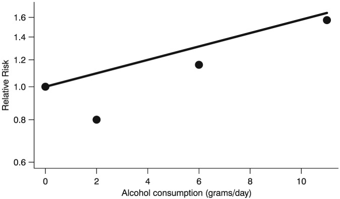
Fitted linear trend (solid line) based on Relative Risks (filled circles) reported in a single study on alcohol consumption and breast cancer risk (Greenland and Longnecker, 1992). Due to the correlation among the Relative Risks, the linear trend does not pass through the data points. The Relative Risks are plotted on the log scale.
To do so, we decompose the covariance matrix S through Cholesky factorization, so that S = CC ′, where C is a lower triangular matrix. We then decorrelate the residuals by multiplying the inverse of C by the difference between reported and fitted log(RR)s, so that . The decorrelated residuals e* are then plotted against the exposure.
The interpretation of this plot is analogous to that of the residual‐versus‐predictor plot that is used as a goodness of fit tool after classic ordinary least squares regression. Although the vertical distances from the reference line are not directly interpretable, from this plot, it is possible to evaluate how the pooled dose–response curve fits the data according to the exposure levels. If the fit is perfect, all the points will lie on the horizontal line e* = 0 (reference line). As the fit gets worse, the points will move away from the reference line. The presence of a pattern might indicate that the fit of the model is adequate only for certain levels of the exposure, suggesting the need of a more complex model. Possible extensions to this plot include overlaying a locally weighted scatterplot smoother (LOWESS) to help discerning possible patterns and, for meta‐regressions, changing the shape of the data points to distinguish them according to study‐level covariates.
3.4. Goodness of fit of study‐specific dose–response models
All the three tools presented so far can be equally employed to assess the goodness of fit of the study‐specific dose–response models (Equation 1). Only minor modifications in the formulas are necessary, which are briefly illustrated in the succeeding text.
The deviance for the ith study is defined as
| (9) |
and when the study‐specific model is correctly specified, it follows a chi‐square distribution with n i − p degrees of freedom. Furthermore, because the K studies are assumed to be independent, it is possible to set up a joint test for model specification for all the K study‐specific models. In fact, under the null hypothesis that all the K models are correctly specified, the sum of the K study‐specific deviances is distributed as a chi‐square random variable with degrees of freedom, that is,
| (10) |
This follows immediately from the fact that the sum of independently distributed chi‐square random variables is again a chi‐square random variable (Forbes et al., 2011).
The coefficient of determination for the ith study is defined as
Lastly, the study‐specific decorrelated residuals are calculated as , where is the inverse of the lower triangular matrix C i obtained from the Cholesky factorization of S i.
4. Examples
We will now illustrate how the deviance, the coefficient of determination, and the residuals‐versus‐exposure plot can help in evaluating and reporting the goodness of fit of dose–response models by using data from two published meta‐analyses. The selected examples are different in terms of number of studies, number of non‐referent log(RR)s, presence of nonlinearity, and/or statistical heterogeneity. We will follow the one‐stage approach to present the meta‐analytical models used in the examples. The complete R code to replicate the results is available at http://github.com/anddis/goodness‐of‐fit‐meta‐analysis.
4.1. Example 1: lactose intake and risk of ovarian cancer
The first example uses data from a meta‐analysis on lactose intake and risk of ovarian cancer (Larsson et al., 2006), including a total of 708 cases among 170 327 participants from three cohort studies and 2253 cases and 3386 controls from six case‐control studies. The analytical dataset comprised therefore nine studies, for a total of 28 non‐referent log(RR)s.
We started by fitting a linear model for the association between the log(RR)s and lactose intake (x ij):
| (11) |
This model was characterized by a particularly poor fit. In particular, the test for model specification showed evidence of lack of fit (D = 41, df = 27, p = 0.04), while the percentage of total variability in the log(RR) explained by model 1 was a mere 1%. Moreover, a large part of between‐study heterogeneity was left unaccounted for (I 2 = 51%) (Table 1). As an additional indication of the poor fit of model 1, the decorrelated residuals of the cohort studies were mostly above 0, while those for case‐control studies were mostly below (Figure 2, panel A). Lastly, the joint test for model specification did not show evidence of lack of fit ( = 24, df = 19, p = 0.18). This might be an indication that study‐specific linear models were indeed adequate to summarize the single dose–response associations. This result strengthened the hypothesis that a study‐level covariate, possibly study design, modified the overall dose–response association.
Table 1.
Goodness of fit and heterogeneity measures for Example 1: lactose intake and risk of ovarian cancer (Larsson et al., 2006).
| Model | Description | Deviance | Degrees of freedoma | p‐valueb | p‐valuec | R 2 (%) | R 2 adj. (%) | Q | Degrees of freedomd | p‐valuee | I 2 (%) |
|---|---|---|---|---|---|---|---|---|---|---|---|
| 1 | Linear model | 41 | 27 | 0.04 | — | 1 | 0 | 16 | 8 | 0.04 | 51 |
| 2 | Linear model + interactionf | 31 | 26 | 0.21 | 0.002 | 24 | 18 | 7 | 7 | 0.43 | 0 |
Degrees of freedom for the deviance statistic.
p‐value from test for model specification.
p‐value for relative goodness of fit with respect to the model on the previous row.
Degrees of freedom for the Q statistic.
p‐value from test for heterogeneity.
Interaction with study‐level binary variable indicating cohort studies versus case‐control studies.
Figure 2.
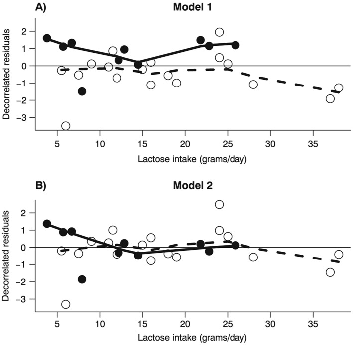
Example 1 (Larsson et al., 2006): decorrelated residuals‐versus‐exposure plots. Decorrelated residuals and LOWESS smoother for Model 1 (Panel A) and for Model 2 (Panel B). Filled circles are the decorrelated residuals of cohort studies; empty circles are the decorrelated residuals for case‐control studies. The solid line is the LOWESS smoother for decorrelated residuals of cohort studies; the dashed line is the LOWESS smoother for decorrelated residuals of case‐control studies.
We therefore employed a meta‐regression model, where we added an interaction term between lactose intake and an indicator variable for the cohort studies (z i):
| (12) |
As a result, the deviance dropped to 31 (D = 31, df = 26, p = 0.21) and the total amount of explained variability in the log(RR), although remained quite low, increased from 1% to 24% (Table 1). The goodness of fit increased significantly relative to model 1 (D = 41–31, df = 27–26, p = 0.002), indicating strong evidence of heterogeneity by study design. Consequently, heterogeneity as measured by I 2 dropped from 51% to 0%. Lastly, the residual‐versus‐exposure plot reflected the improved fit of model 2 (Figure 2, panel B). The pooled RR for every 10 g/day of lactose intake was (95% confidence interval: 0.91, 1.03) for case‐control studies and (95% confidence interval: 1.05, 1.25) for cohort studies. The low overall R 2 coefficient (24%) was due to the lack of association among case‐control studies. On the other hand, the R 2 among the cohort studies indicated an acceptable agreement between observed and fitted log(RR)s (R 2 = 53%).
4.2. Example 2: coffee consumption and risk of stroke
The second example concerns a meta‐analysis on coffee consumption and risk of stroke, including 10 003 cases and 479 689 participants from 11 cohort studies (Larsson and Orsini, 2011). A total of 52 non‐referent log(RR)s were available for the analysis.
We started by considering a linear model for coffee consumption (model 1), which fitted the data poorly, as indicated by a deviance of 140 on 51 df (p < 0.001) (Table 2). The residual‐versus‐exposure plot showed that the fit of the model was unsatisfactory, particularly for higher levels of coffee consumption (Figure 3, panel A). Moreover, model 1 explained only a minimal amount of between‐study heterogeneity (I 2 = 80%).
Table 2.
Goodness of fit and heterogeneity measures for Example 2: coffee consumption and risk of stroke (Larsson and Orsini, 2011).
| Model | Description | Deviance | Degrees of freedoma | p‐valueb | p‐valuec | R 2 (%) | R 2 adj. (%) | Q | Degrees of freedomd | p‐valuee | I 2 (%) |
|---|---|---|---|---|---|---|---|---|---|---|---|
| 1 | Linear model | 140 | 51 | <0.001 | — | 41 | 39 | 76 | 15 | <0.001 | 80 |
| 2 | Restricted cubic spline model | 75 | 50 | 0.01 | <0.001 | 68 | 67 | 54 | 30 | 0.005 | 44 |
| 3 | Restricted cubic spline model + interactionf | 64 | 48 | 0.06 | 0.005 | 73 | 70 | 44 | 28 | 0.03 | 36 |
Degrees of freedom for the deviance statistic.
p‐value from test for model specification.
p‐value for relative goodness of fit with respect to the model on the previous row.
Degrees of freedom for the Q statistic.
p‐value from test for heterogeneity.
Interaction with study‐level binary variable indicating studies conducted in the Nordic countries versus studies conducted elsewhere.
Figure 3.
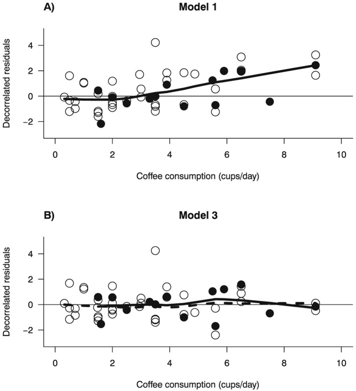
Example 2 (Larsson and Orsini, 2011): decorrelated residuals‐versus‐exposure plots. Filled circles are the decorrelated residuals of studies conducted in the Nordic countries; empty circles are the decorrelated residuals for studies conducted elsewhere. The solid line is the LOWESS smoother for decorrelated residuals of studies conducted in the Nordic countries; the dashed line is the LOWESS smoother for decorrelated residuals of studies conducted elsewhere.
To address the lack of fit of model 1, we modeled coffee consumption using RCS with three knots at fixed percentiles (25%, 50%, and 75%) of the exposure distribution:
| (2) |
where x ij1 and x ij2 are the two RCS transformations of coffee consumption. The improvement in the goodness of fit of the RCS model was reflected by the increase in the R 2 coefficient from 41% to 68%, and by the large difference in the deviances between model 1 and model 2 (D = 140–75 = 65, df = 51–50, p < 0.001) (Table 2).
We next investigated whether a possible interaction between coffee consumption and study location could at least partly explain the statistical heterogeneity and provide a better fit of the log(RR)s. Therefore, we added to model 2 the interactions terms between the two RCS transformations and a dummy variable (z i) identifying the four studies conducted in the Nordic countries (Sweden and Finland):
| (3) |
The deviance decreased to 64 on 48 df (p = 0.06), while the percentage of total explained variability increased to R 2 = 73%. Even after introducing a penalty term for the two extra parameters to be estimated, model 3 fitted the data better than model 2 as indicated by the (70% vs. 67%). Moreover, the residuals‐versus‐exposure plot no longer showed indication of lack of fit at high exposure levels (Figure 3, panel B). Finally, the test for heterogeneity of the dose–response relation between the two groups of studies was statistically significant (D = 75–64, df = 50–48, p = 0.005), and heterogeneity decreased to I 2 = 36% (Table 2). Using nondrinkers as the reference group, the estimated dose–response relation between coffee consumption and relative risk of stroke for the studies conducted in the Nordic countries (z i = 1) was , while for the studies conducted elsewhere (z i = 0), it was (Figure 4). Lastly, we calculated the RR for individuals who drank eight cups per day versus nondrinkers. The values of the first and second RCS transformation for a coffee consumption of eight cups per day were x ij1 = 8 and x ij2 = 8.2, respectively. Therefore, for the studies conducted in the Nordic countries, the estimated RR was exp(−0.079 × 8 + 0.04 × 8.2) = 0.74, while it was exp(−0.087 × 8 + 0.077 × 8.2) = 0.94 for the studies conducted elsewhere.
Figure 4.
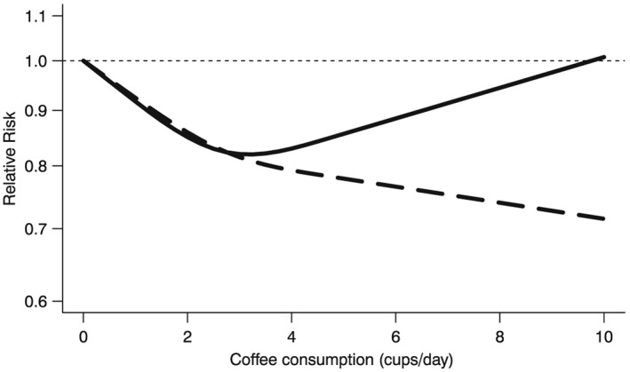
Example 2 (Larsson and Orsini, 2011): pooled dose‐response relation between coffee consumption (cups/day) and risk of stroke from Model 3 for studies conducted in the Nordic countries (dashed line) and for studies conducted elsewhere (solid line). The Relative Risks are plotted on the log scale.
Overall, even though a large amount of variability in the log(RR)s was explained, there was still some evidence that the remaining variability was larger than one would expect if model 3 was indeed correctly specified (p = 0.06). Moreover, even after accounting for study location via meta‐regression, remaining between‐study heterogeneity was still significant (p = 0.03). Therefore, one might think that a better fitting model is needed.
5. Discussion
The main objective of this paper was to present and discuss three tools (deviance, coefficient of determination, and decorrelated residuals‐versus‐exposure plot) that can be used for testing, quantifying, and visually displaying the fit of dose–response meta‐analytical models. To the best of our knowledge, the R 2 coefficient and the decorrelated residuals‐versus‐exposure plot have never been used in the context of dose–response meta‐analysis. Furthermore, we reviewed the methods employed in the estimation of fixed‐effects dose–response meta‐analysis and showed analytically that one‐stage and two‐stage approaches are equivalent.
To illustrate how these tools can be applied in practice, we reanalyzed data from two published meta‐analyses that differed in terms of presence of nonlinearity and/or heterogeneity. These examples showed how careful scrutiny of the candidate models using the tools presented in this paper can give important indications regarding their fit.
The tools presented in this paper can be equally employed to assess the adequacy of the study‐specific models. This can be potentially useful to further examine the dose–response relation and to investigate how its shape changes across studies, thus helping to identify sources of heterogeneity. However, one limitation related to this use of the proposed tools is that the number of non‐referent log(RR) estimates reported by the single studies is generally small. As a result, the ability to assess the study‐specific models' goodness of fit is often limited.
The decorrelated residuals‐versus‐exposure plot is extendable to random‐effects dose–response models by including the covariance matrix of the random effects in the Cholesky factorization (Fitzmaurice et al., 2011). On the other hand, deviance and coefficient of determination R 2 are motivated via the fixed‐effects framework and lack a direct equivalent for random‐effects models. Their use for diagnostic purposes is, however, independent of the inclusion of random effects in the final model.
In conclusion, we think that the use of the goodness of fit tools presented in this paper can improve the practice of quantitative review of aggregated dose–response data. In fact, they can help the identification of dose–response patterns, the investigation of sources of heterogeneity, and the assessment of whether the pooled dose–response relation adequately summarizes the published results. By doing so, their use can yield important insights that either strengthen the conclusions drawn from a dose–response meta‐analysis, or, conversely, raise doubts about its ability to adequately summarize the available evidence.
Supporting information
Supporting info item
Acknowledgements
The authors would like to thank two anonymous reviewers for their useful comments that contributed to improve the final version of the paper.
This work was supported by Karolinska Institutet's funding for doctoral students (KID‐funding) (A.D. and A.C.) and by a Young Scholar Award from the Karolinska Institutet's Strategic Program in Epidemiology (SfoEpi) (N.O.).
Discacciati, A. , Crippa, A. , and Orsini, N. (2017) Goodness of fit tools for dose–response meta‐analysis of binary outcomes. Res. Syn. Meth., 8: 149–160. doi: 10.1002/jrsm.1194.
References
- Bagnardi V, Zambon A, Quatto P, Corrao G 2004. Flexible meta‐regression functions for modeling aggregate dose–response data, with an application to alcohol and mortality. American Journal of Epidemiology 159: 1077–1086. [DOI] [PubMed] [Google Scholar]
- Berkey CS, Hoaglin DC, Antczak‐Bouckoms A, Mosteller F, Colditz GA 1998. Meta‐analysis of multiple outcomes by regression with random effects. Statistics in Medicine 17: 2537–2550. [DOI] [PubMed] [Google Scholar]
- Berlin JA, Longnecker MP, Greenland S 1993. Meta‐analysis of epidemiologic dose–response data. Epidemiology (Cambridge, Mass.) 4: 218–228. [DOI] [PubMed] [Google Scholar]
- Buse A 1973. Goodness of fit in generalized least squares estimation. American Statistician 27: 106–108. [Google Scholar]
- Cochran WG 1954. The combination of estimates from different experiments. Biometrics 10: 101–129. [Google Scholar]
- Draper NR, Smith H 1998. Applied Regression Analysis. Third ed. edn.John Wiley & Sons: Hoboken, New Jersey. [Google Scholar]
- Eisenhauer JG 2003. Regression through the origin. Teaching Statistics 25: 76–80. [Google Scholar]
- Fitzmaurice GM, Laird NM, Ware JH 2011. Applied Longitudinal Analysis. Second ed edn.John Wiley & Sons: Hoboken, New Jersey. [Google Scholar]
- Forbes C, Evans M, Hastings N, Peacock B 2011. Statistical Distributions. Fourth ed edn.John Wiley & Sons: Hoboken, New Jersey. [Google Scholar]
- Fu Y‐Q, Zheng J‐S, Yang B, Li D 2015. Effect of individual omega‐3 fatty acids on the risk of prostate cancer: a systematic review and dose–response meta‐analysis of prospective cohort studies. Journal of the Epidemiology/Japan Epidemiological Association 25: 261–274. [DOI] [PMC free article] [PubMed] [Google Scholar]
- Gasparrini A, Armstrong B, Kenward MG 2012. Multivariate meta‐analysis for non‐linear and other multi‐parameter associations. Statistics in Medicine 31: 3821–3839. [DOI] [PMC free article] [PubMed] [Google Scholar]
- Greenland S, Longnecker MP 1992. Methods for trend estimation from summarized dose–response data, with applications to meta‐analysis. American Journal of Epidemiology 135: 1301–1309. [DOI] [PubMed] [Google Scholar]
- Hagquist C, Stenbeck M 1998. Goodness of fit in regression analysis – R 2 and G 2 reconsidered. Quality and Quantity 32: 229–245. [Google Scholar]
- Hahn GJ 1977. Fitting regression models with no intercept term. Journal of Quality Technology 9: 56–61. [Google Scholar]
- Hamling J, Lee P, Weitkunat R, Ambühl M 2008. Facilitating meta‐analyses by deriving relative effect and precision estimates for alternative comparisons from a set of estimates presented by exposure level or disease category. Statistics in Medicine 27: 954–970. [DOI] [PubMed] [Google Scholar]
- Hardy RJ, Thompson SG 1998. Detecting and describing heterogeneity in meta‐analysis. Statistics in Medicine 17: 841–856. [DOI] [PubMed] [Google Scholar]
- Harrell FE 2001. Regression Modeling Strategies: With Applications to Linear Models, Logistic Regression, and Survival Analysis. New York, NY: Springer. [Google Scholar]
- Jackson D, White IR, Riley RD 2012. Quantifying the impact of between‐study heterogeneity in multivariate meta‐analyses. Statistics in Medicine 31: 3805–3820. DOI:10.1002/sim.5453. [DOI] [PMC free article] [PubMed] [Google Scholar]
- Kvålseth TO 1985. Cautionary note about R 2 . American Statistician 39: 279–285. [Google Scholar]
- Larsson SC, Orsini N 2011. Coffee consumption and risk of stroke: a dose–response meta‐analysis of prospective studies. American Journal of Epidemiology 174: 993–1001. [DOI] [PubMed] [Google Scholar]
- Larsson SC, Orsini N, Wolk A 2006. Milk, milk products and lactose intake and ovarian cancer risk: a meta‐analysis of epidemiological studies. International Journal of Cancer 118: 431–441. [DOI] [PubMed] [Google Scholar]
- Liao W‐C, Tu Y‐K, Wu M‐S, Lin J‐T, Wang H‐P, Chien K‐L 2015. Blood glucose concentration and risk of pancreatic cancer: systematic review and dose–response meta‐analysis. BMJ 349: g7371. [DOI] [PMC free article] [PubMed] [Google Scholar]
- Liu Q, Cook NR, Bergström A, Hsieh C‐C 2009. A two‐stage hierarchical regression model for meta‐analysis of epidemiologic nonlinear dose–response data. Computational Statistics and Data Analysis 53: 4157–4167. [Google Scholar]
- Orsini N, Bellocco R, Greenland S 2006. Generalized least squares for trend estimation from summarized dose–response data. Stata Journal 6: 40–57. [Google Scholar]
- Orsini N, Li R, Wolk A, Khudyakov P, Spiegelman D 2012. Meta‐analysis for linear and nonlinear dose–response relations: examples, an evaluation of approximations, and software. American Journal of Epidemiology 175: 66–73. [DOI] [PMC free article] [PubMed] [Google Scholar]
- Ritz J, Demidenko E, Spiegelman D 2008. Multivariate meta‐analysis for data consortia, individual patient meta‐analysis, and pooling projects. The Journal of Statistical Planning and Inference 138: 1919–1933. [Google Scholar]
- Rota M, Bellocco R, Scotti L, Tramacere I, Jenab M, Corrao G, La Vecchia C, Boffetta P, Bagnardi V 2010. Random‐effects meta‐regression models for studying nonlinear dose–response relationship, with an application to alcohol and esophageal squamous cell carcinoma. Statistics in Medicine 29: 2679–2687. [DOI] [PubMed] [Google Scholar]
- Shi JQ, Copas JB 2004. Meta‐analysis for trend estimation. Statistics in Medicine 23: 3–19; discussion 159–162. [DOI] [PubMed] [Google Scholar]
- Sun J‐W, Zhao L‐G, Yang Y, Ma X, Wang Y‐Y, Xiang Y‐B 2015. Obesity and risk of bladder cancer: a dose–response meta‐analysis of 15 cohort studies. PloS One 10, e0119313. [DOI] [PMC free article] [PubMed] [Google Scholar]
- Sutton AJ, Higgins JPT 2008. Recent developments in meta‐analysis. Statistics in Medicine 27: 625–650. DOI:10.1002/sim.2934. [DOI] [PubMed] [Google Scholar]
- Takahashi K, Nakao H, Hattori S 2013. Cubic spline regression of J‐shaped dose–response curves with likelihood‐based assignments of grouped exposure levels. Journal of Biometrics & Biostatistics 4: 181. [Google Scholar]
- Takahashi K, Tango T 2010. Assignment of grouped exposure levels for trend estimation in a regression analysis of summarized data. Statistics in Medicine 29: 2605–2616. [DOI] [PubMed] [Google Scholar]
- Theil H 1961. Economic Forecasts and Policy. Amsterdam: North‐Holland Publishing Company. [Google Scholar]
- van Houwelingen HC, Arends LR, Stijnen T 2002. Advanced methods in meta‐analysis: multivariate approach and meta‐regression. Statistics in Medicine 21: 589–624. [DOI] [PubMed] [Google Scholar]
- Xu C, Zeng X‐T, Liu T‐Z, Zhang C, Yang Z‐H, Li S, Chen X‐Y 2015. Fruits and vegetables intake and risk of bladder cancer: a PRISMA‐compliant systematic review and dose–response meta‐analysis of prospective cohort studies. Medicine (Baltimore) 94: e759. [DOI] [PMC free article] [PubMed] [Google Scholar]
- Xu W, Tan L, Wang H‐F, Tan M‐S, Tan L, Li J‐Q, Zhao Q‐F, Yu J‐T 2015. Education and risk of dementia: dose–response meta‐analysis of prospective cohort studies. Molecular Neurobiology. [DOI] [PubMed] [Google Scholar]
Associated Data
This section collects any data citations, data availability statements, or supplementary materials included in this article.
Supplementary Materials
Supporting info item