Design of nucleic acid sequences for DNA computing based on a thermodynamic approach

Abstract

We have developed an algorithm for designing multiple sequences of nucleic acids that have a uniform melting temperature between the sequence and its complement and that do not hybridize non-specifically with each other based on the minimum free energy (ΔG_min). Sequences that satisfy these constraints can be utilized in computations, various engineering applications such as microarrays, and nano-fabrications. Our algorithm is a random generate-and-test algorithm: it generates a candidate sequence randomly and tests whether the sequence satisfies the constraints. The novelty of our algorithm is that the filtering method uses a greedy search to calculate ΔG_min. This effectively excludes inappropriate sequences before ΔG_min is calculated, thereby reducing computation time drastically when compared with an algorithm without the filtering. Experimental results in silico showed the superiority of the greedy search over the traditional approach based on the hamming distance. In addition, experimental results in vitro demonstrated that the experimental free energy (ΔG_exp) of 126 sequences correlated well with ΔG_min (|R| = 0.90) than with the hamming distance (|R| = 0.80). These results validate the rationality of a thermodynamic approach. We implemented our algorithm in a graphic user interface-based program written in Java.

INTRODUCTION

Nucleic acids are now being utilized in computations (1–3), various engineering applications such as microarrays (4–6), and nano-fabrications (7–9). In these fields of research, called ‘DNA computing’, nucleic acid design or sequence design is a crucial problem in engineering using nucleic acids. Nucleic acid design is deciding the base sequences (e.g. ‘GCTAGCTAGGTTTA’,…,‘ATCGTACGCTATGTGCA’ in DNA) in order to satisfy the constraints based on the physicochemical properties of nucleic acids. In particular, it is essential to prevent undesired hybridization. In DNA computing, multiple sequences need to be designed that do not hybridize non-specifically with each other (10,11), while in RNA secondary structure design, a single sequence needs to be designed that folds into the desired secondary structure (12–15). For example, 40 DNA sequences of length 15 were designed to prevent undesired hybridization and used for solving a 20-variable instance of a three-satisfiability problem (2). In the field of microarrays, 69 122 DNA sequences of length 45–47 were designed to hybridize specifically to 24 502 transcripts from Arabidopsis thaliana (4). Furthermore, four DNA sequences of length 26 and four DNA sequences of length 48 were used to construct a periodic two-dimensional crystalline lattice (7). These sequences were carefully designed for the intended hybridization. Thus, an algorithm/program that generates multiple sequences, which do not hybridize non-specifically with each other, is useful for various applications of nucleic acid.

We applied a thermodynamic approach to the nucleic acid design for DNA computing. In particular, we focused on designing a pool P containing n sequences of length l for which (i) the duplex melting temperature (T_M) is in the range $T_{\text{M}}^{-}$ to $T_{\text{M}}^{+}$ for any pairwise duplex of a sequence in P and its complement and (ii) the minimum free energy (ΔG_min) is greater than a threshold ($\Delta G_{\text{min}}^{*}$) in any pairwise duplex of sequences in P and any concatenation of two sequences in P plus their complements except for the pairwise duplex of a sequence in P and its complement. Traditional approaches to the sequence design in DNA computing have approximated the stability between two sequences using the hamming distance (i.e. the number of base pairs) rather than ΔG_min. However, since the hamming distance is only an approximation of the stability, ΔG_min is preferable for predicting the stability. In practice, an RNA secondary structure can be adequately predicted using ΔG_min rather than the number of base pairs (16). However, the algorithm for calculating the ΔG_min for double-stranded DNA requires time complexity O(l³), where l is the length of the sequence, as is the case with secondary structure prediction for single-stranded RNA. Since all the combinations of three sequences must be evaluated in this design, dozens of sequences cannot be designed within a reasonable computation time. Another approach that reduces the computation time is thus needed. Andronescu et al. (13) overcame this drawback in the secondary structure design by hierarchically decomposing the secondary structure into smaller substructures and integrating the partial sequences. By using this method, they designed sequences that a traditional program cannot.

We have developed a random generate-and-test algorithm that generates a candidate sequence randomly and tests whether the sequence satisfies the constraints. It stores the sequence in a sequence pool if and only if it satisfies all the constraints. To reduce the difficulty in computation time, we use a greedy search to calculate ΔG_min. The advantage of a greedy search is that it approximates ΔG_min in less time, with time complexity O(l²), than a rigorous algorithm, which calculates ΔG_min with time complexity O(l³). The ΔG_min approximated using the greedy search (denoted by ΔG_gre) correlated well with ΔG_min. The correlation coefficients were 0.95, 0.85 and 0.76 at 20mer, 40mer and 60mer lengths, respectively. Furthermore, since ΔG_gre is the upper bound for ΔG_min (i.e. ΔG_min≤ΔG_gre), the sequence such that $\Delta G_{\text{gre}}\le \Delta G_{\text{min}}^{*}$ is sure to satisfy $\Delta G_{\text{min}}\le \Delta G_{\text{min}}^{*}$. Therefore, using a greedy search excludes in advance most inappropriate sequences before ΔG_min is calculated without excluding an appropriate sequence. With this approach, our algorithm reduces computation time.

To evaluate our algorithm, we investigated the effectiveness of the greedy search filtering. We compared the computation time of our algorithm with that of the same algorithm but without the greedy search filtering. The experimental results showed that the greedy search filtering reduces the total computation time drastically. For example, using the filtering reduced the computation time to 83% for 30 sequences with length 20 and to 87% for 20 sequences with length 15 when $T_{\text{M}}^{-}=69.58$, $T_{\text{M}}^{+}=72.58$ and $\Delta G_{\text{min}}^{*}=-10.0$, and $T_{\text{M}}^{-}=60.49$, $T_{\text{M}}^{+}=63.49$ and $\Delta G_{\text{min}}^{*}=-7.0$, respectively. In addition, we compared the greedy search with the traditional approach based on a hamming distance in terms of the filtering performance. We demonstrated that the greedy search can filter out inappropriate sequences better than using the hamming distance. In a laboratory experiment, we investigated the correlation coefficient between ΔG_min and the experimental free energy (ΔG_exp) and that between the hamming distance and the ΔG_exp using 126 duplexes. The ΔG_exp correlated better with ΔG_min (|R| = 0.90) than with the hamming distance (|R| = 0.80).

To implement our algorithm, we developed a computer program called DNA-SDT, a graphic user interface (GUI)-based application written in Java. This program enables users to design DNA sequences with our algorithm and can be downloaded freely from the web site (http://ses3.complex.eng.hokudai.ac.jp/~fumi95/DNA-SDT/index.html).

ALGORITHM

Definition

Let n be the number of sequences to be designed and l_i (0 ≤ i ≤ n − 1) be the length of each sequence. In this paper, we formulated l_i such that l_i = l_j = l (0 ≤ i, j ≤ n − 1), although we can extend our algorithm easily for l_i ≠ l_j (0 ≤ i ≠ j ≤ n − 1). We define P as the pool of n sequences, with length l, to be designed. Furthermore, let P = {U₀, U₁,…, U_n−1} and Q = {V₀, V₁,…, V_n−1} such that V_i (0 ≤ i ≤ n − 1) is the complement of U_i. $T_{\text{M}}^{-}$ and $T_{\text{M}}^{+}$ are defined as the lower and upper thresholds of T_M for the duplex between a sequence and its complement. Moreover, $\Delta G_{\text{min}}^{*}$ is defined as the threshold of ΔG_min given by the sequence designer. Thus, our algorithm designs a pool P containing n sequences of length l for which (i) the duplex T_M is in the range from $T_{\text{M}}^{-}$ to $T_{\text{M}}^{+}$ for any duplex of U_i (0 ≤ i ≤ n − 1) and V_i, and (ii) ΔG_min is greater than $\Delta G_{\text{min}}^{*}$ for any pairwise duplex of sequences in P and any concatenation of two sequences in P ∪ Q except for the pairwise duplex of U_i and V_i.

Here, we describe more specifically the combination of sequences to be calculated using the ΔG_min. The sequence U_i (0 ≤ i ≤ n − 1) is denoted by a string of bases such as $u_i^0{u}_i^1\cdots u_i^{l-1}$ (5′ to 3′ direction), and similarly, V_i (0 ≤ i ≤ n − 1) is denoted as $v_i^0{v}_i^1\cdots v_i^{l-1}$ (5′ to 3′ direction). For example, if U_i = 5′-AAATTTCCCGGG-3′, then V_i = 5′-CCCGGGAAATTT-3′. Furthermore, let 〈X, Y〉 be the combination of sequences X and Y, and XY be the concatenation of sequences X and Y in that order. For example, if U_i, U_j and U_k (0 ≤ i, j, k ≤ n − 1) are 5′-AAATTT-3′, 5′-CCCGGG-3′ and 5′-TCTCTC-3′, respectively, then 〈U_iU_j,U_k〉 means the combination of sequences 5′-AAATTTCCCGGG-3′ and 5′-TCTCTC-3′. In our algorithm, the following combinations are considered for the ΔG_min calculation.

1. 〈U_i U_j U_k 〉 (0 ≤ i, j, k ≤ n − 1)

2. 〈U_i U_j V_k 〉 (0 ≤ i, j, k ≤ n − 1), i ≠ k

3. 〈U_i V_j U_k 〉 (0 ≤ i, j, k ≤ n − 1), i ≠ j

4. 〈U_i V_j V_k 〉 (0 ≤ i, j, k ≤ n − 1), (i ≠ j)∧(i ≠ k).

For generality, we use two sequences, S(=s₀s₁⋯s_N−1) (5′ to 3′ direction) and T(=t₀ t₁⋯t_M−1) (3′ to 5′ direction), to describe the ΔG_min calculation in detail. The sequences are defined to be antiparallel to each other. Note that any two sequences can be represented by S and T. In this paper, S and T represent U_i and the reverse sequence of X_jY_k (X_j ∈ {U_j, V_j}, X_k ∈ {U_k, V_k}).

The notation s_i · t_j represents the base pair between the i-th base in sequence S and the j-th base in sequence T, hence the structure between S and T is a set of base pairs such that each base is paired at most once. In addition, (s_i · t_j, s_i′ · t_j′) $\left\{\right(0\le i<i^{\prime }\le N-1)\wedge (0\le j<j^{\prime }\le M-1\left)\right\}$ is defined as a structure in which base pairs s_i · t_j and s_i′ · t_j′ are formed and the sequences $s_{i+1}{s}_{i+2}\cdots s_{i^{\prime }-1}$ and $t_{j+1}{t}_{j+2}\cdots t_{j^{\prime }-1}$ do not form any base pairs. The term $(x,s_{i^{\prime }}·t_{j^{\prime }})$ $\{x\in \{s_i,t_j\},(0\le i<i^{\prime }\le N-1)\wedge (0\le j<j^{\prime }\le M-1\left)\right\}$ is defined as a structure in which base pair s_i′ · t_j′ is formed and sequence $s_i{s}_{i+1}\cdots s_{i^{\prime }-1}$ in the case $x=s_i$ ($t_j{t}_{j+1}\cdots t_{j^{\prime }-1}$ in the case $x=t_j$) do not form any base pair. Similarly, $(s_i·t_j,x)$ $\{x\in \{s_{i^{\prime }},t_{j^{\prime }}\},(0\le i<i^{\prime }\le N-1)\wedge (0\le j<j^{\prime }\le M-1\left)\right\}$ is defined as a structure in which base pair s_i · t_j is formed and the sequence $s_{i+1}{s}_{i+2}\cdots s_{i^{\prime }}$ in the case $x=s_{i^{\prime }}$ ($t_{j+1}{t}_{j+2}\cdots t_{j^{\prime }}$ in the case $x=t_{j^{\prime }}$) do not form any base pair.

Outline

Our algorithm is a random generate-and-test algorithm that generates a sequence randomly and then stores it in the pool if and only if the sequence satisfies all the constraints. The main feature of our algorithm is that it uses a greedy search for calculating ΔG_min to filter out inappropriate sequences. The advantage of a greedy search is that it approximates ΔG_min in less time when compared with a well-known dynamic programming algorithm (17). Therefore, using the greedy search before the ΔG_min calculation to exclude inappropriate sequences reduces the computation time. Hereafter, the approximated ΔG_min using a greedy search is denoted by ΔG_gre.

The algorithm uses three filters:

1. T_M filter: checks whether the T_M of candidate sequence U_c $(0\le c\le n-1)$ and V_c is in the range from $T_{\text{M}}^{-}$ to $T_{\text{M}}^{+}$. If not, U_c is rejected.

2. ΔG_gre filter: checks whether ΔG_gre is greater than the threshold, $\Delta G_{\text{gre}}^{*}$, for all the combinations above in P, provided that the candidate sequence U_c $(0\le c\le n-1)$ or V_c is included in that combination. If the ΔG_gre of any combination is less than or equal to $\Delta G_{\text{gre}}^{*}$, U_c is rejected.

3. ΔG_min filter: checks whether ΔG_min is greater than the threshold, $\Delta G_{\text{min}}^{*}$, for all the combinations above in P, provided that the candidate sequence U_c $(0\le c\le n-1)$ or V_c is included in that combination. If the ΔG_min of any combination is less than or equal to $\Delta G_{\text{min}}^{*}$, U_c is rejected.

The T_M and ΔG_min filters are necessary for satisfying the constraints of sequence design, while the ΔG_gre filter reduces the computation time. The use of the ΔG_gre filter is based on the hypothesis that it can exclude most sequences that cannot pass through the ΔG_min filter. If this hypothesis is true, the ΔG_gre filter can exclude the inappropriate sequences in less time, resulting in reduced total computation time.

The algorithm is defined as follows:

• Input: n, l, $T_{\text{M}}^{-}$, $T_{\text{M}}^{+}$, $\Delta G_{\text{gre}}^{*}$, $\Delta G_{\text{min}}^{*}$

• Output: pool P consisting of n sequences with length l.

• Procedure:

  1. Initialize pool P as an empty set.
  2. Iterate the following procedure until P has n sequences.

     1. Generate candidate sequence U_c $\left(0\le c\le n-1\right)$ with length l randomly, then add U_c to P.
     2. Evaluate U_c with T_M filter. If U_c is rejected, exclude U_c from P and return to ii(a).
     3. Evaluate U_c with ΔG_gre filter. If U_c is rejected, exclude U_c from P and return to ii(a).
     4. Evaluate U_c with ΔG_min filter. If U_c passes, leave U_c in P; else exclude U_c from P and return to ii(a).

The order of the filters is important. Each candidate sequence should be evaluated in this order to reduce the computation time. If pool P has m sequences, the time complexities to evaluate the (m + 1)-th candidate sequence are O(l), O(m²l²) and O(m²l³) at the T_M, ΔG_gre and ΔG_min filters, respectively. By evaluating the candidate sequences in ascending order of time complexity, the inappropriate ones can be excluded sooner.

Energy model

The ΔG_min between S and T is calculated using a dynamic programming algorithm (17), while the ΔG_gre between S and T is calculated using a greedy search. Both ΔG_min and ΔG_gre are calculated based on the nearest-neighbor model, which calculates the total free energy as the summation of the contributions of various elementary structures (18,19). The elementary structures considered in this paper are stacking base pairs, bulge loops, internal loops, dangling ends and free ends.

The contributions of the stacking base pairs, defined as $(s_i·t_j,s_{i+1}·t_{j+1})$, to the free energy are calculated using 12 parameters reported previously (19). The free energy contributions of the loop regions are sequence dependent (15,16,20). The free energies of single bulge loops, defined as $(s_i·t_j,s_{i+2}·t_{j+1})$ or $(s_i·t_j,s_{i+1}·t_{j+2})$, are calculated using 64 parameters covering all the possible combinations of bulged base and flanking base pairs (19). The free energies of the other loops, bulge loops longer than one and internal loops, are calculated using conventional parameters and equations (20,21). Bulge loops longer than one are defined as $\left\{(s_i·t_j,s_{i+l}·t_{j+1})\wedge (l\ge 3)\right\}$ or $(s_i·t_j,s_{i+1}·t_{j+l})\wedge (l\ge 3)$, and the internal loops are defined as $(s_i·t_j,s_{i+l}·t_{j+m})\wedge (l,m\ge 2)$. The free energies of dangling ends, defined as $(s_0,s_1·t_0)$, $(t_0,s_0·t_1)$, $(s_{N-2}·t_{M-1},s_{N-1})$ or $(s_{N-1}·t_{M-2},t_{M-1})$, are calculated using 32 parameters covering all the possible combinations (22). The free ends are defined as the sequences $s_0\cdots s_i$ and $t_0\cdots t_j$ closing with $s_i·t_j$ such that both $s_{i^{\prime }(<i)}$ and $t_{j^{\prime }(<j)}$ do not form a base pair or $s_i\cdots s_{N-1}$ and $t_j\cdots t_{M-1}$ closing with $s_i·t_j$ such that both $s_{(i<)i^{\prime }}$ and $t_{(j<)j^{\prime }}$ do not form a base pair. The free energies of the free ends are also calculated using conventional parameters (20).

The crossing base pairs are defined as a pair of base pairs $s_i·t_j$ and $s_{i\prime }·t_{j\prime }$ in a structure with {(i < i′) ∧ (j′ < j)} or {(i′ < i) ∧ (j < j′)}. We prohibit crossing base pairs because of the computation time and the lack of thermodynamic data. This constraint is equivalent to the pseudoknot-free constraint in the RNA secondary structure prediction. At this point, we do not consider intra-molecular base pairs or the interactions between loop regions.

T_M filter

This filter checks whether a candidate sequence paired to its complement has a T_M in the range $T_{\text{M}}^{-}$ to $T_{\text{M}}^{+}$.

$$T_{\text{M}}=\frac{\Delta H^{°}}{Rln(C_{\text{T}}/\alpha )}+\Delta S^{°},$$ 1

where R is the gas constant, C_T is the concentration, ΔH° is the enthalpy and ΔS° is the entropy. Parameter α is set to 1 for self-complementary and to 4 for non-self-complementary. Parameters ΔH° and ΔS° are calculated based on the nearest-neighbor model (18,19).

ΔG_gre filter

This filter checks whether ΔG_gre is greater than $\Delta G_{\text{gre}}^{*}$ for all the combinations as mentioned in Algorithm.

Using a ‘greedy search’ reduces the computation time for calculating ΔG_min. The greedy search works well because a structure with ΔG_min tends to include stable helices (i.e. continuous complementary regions). Therefore, the greedy search approximates ΔG_min by iteratively searching for the most stable helix and fixing the helix.

The greedy search algorithm is as follows:

1. First, calculate the free energies of all helices over the structure between sequence $s_0{s}_1\cdots s_{N-1}$ and sequence $t_0{t}_1\cdots t_{M-1}$. Calculate the free energies of the helices with free ends using the following equations. Here, a helix is denoted by $s_i{s}_{i+1}\cdots s_k$ (5′ → 3′) and $t_j{t}_{j+1}\cdots t_{l(=j+k-i)}$ (3′ → 5′).

   • $\Delta G_{\text{freeEnd}}=\Delta G_{\text{core}}+D(s_0,s_i,t_0,t_j)+D(t_{M-1},t_l,s_{N-1},s_k)$
   • $\Delta G_{\text{core}}={\sum }_{a=i}^{k-1}eS(s_a,s_{a+1},t_{j+a-i},t_{j+a-i+1})$

   ΔG_freeEnd is the free energy of a helix with free ends; ΔG_core is that without free ends. $D(s_0,s_i,t_0,t_j)$ represents the free energy contribution of the dangling or free end between sequence $5^{\prime }\text{-}{s}_0{s}_1\cdots s_i\text{-}{3}^{\prime }$ and sequence $3^{\prime }\text{-}{t}_0{t}_1\cdots t_j\text{-}{5}^{\prime }$ closing with base pair $s_i·t_j$. For $(i=0)\wedge (j=0)$, $D(s_0,s_i,t_0,t_j)$ is zero because there is no dangling or free end. $eS(s_a,s_{a+1},t_{j+a-i},t_{j+a-i+1})$ is the free energy of the stacked base pair between sequence $5^{\prime }\text{-}{s}_a{s}_{a+1}\text{-}{3}^{\prime }$ and sequence $3^{\prime }\text{-}{t}_{j+a-i}{t}_{j+a-i+1}\text{-}{5}^{\prime }$.

2. Search for a minimal value of ΔG_freeEnd over all helices. Then, fix the base pairs in the helix where ΔG_freeEnd is minimum. This region is freshly denoted as $s_i{s}_{i+1}\cdots s_k$ (5′ → 3′) and $t_j{t}_{j+1}\cdots t_{l(=j+k-i)}$ (3′ → 5′). Furthermore, the free energies of the regions with and without free ends are freshly denoted as ΔG_freeEnd and ΔG_core, respectively.

3. Iterate the following procedure d times, where d is a parameter defined below.

   1. If $(0<i-1)\wedge (0<j-1)$ holds, calculate the free energies of all helices with the loop closing with base pair $s_i·t_j$ over the structure between sequence $s_0{s}_1\cdots s_{i-1}$ and the sequence $t_0{t}_1\cdots t_{j-1}$. Thus, the free energy of helix, denoted as $s_{i^{\prime }}{s}_{i^{\prime }+1}\cdots s_{k^{\prime }}$ (5′ → 3′) and $t_{j^{\prime }}{t}_{j^{\prime }+1}\cdots t_{l^{\prime }(=j^{\prime }+k^{\prime }-i^{\prime })}$ (3′ → 5′), is calculated as follows:

      • $\Delta G_{\text{freeEnd}}^L=\Delta G_{\text{core}}^L+D(s_0,s_{i^{\prime }},t_0,t_{j^{\prime }})$
      • $\Delta G_{\text{core}}^L={\sum }_{a=i^{\prime }}^{k^{\prime }-1}eS(s_a,s_{a+1},t_{j^{\prime }+a-i^{\prime }},t_{j^{\prime }+a-i^{\prime }+1})+eL(s_{k^{\prime }},s_i,t_{l^{\prime }},t_j),$

      where $\Delta G_{\text{freeEnd}}^L$ is the free energy of the helix with a free end, $\Delta G_{\text{core}}^L$ is that of one without a free end and $eL(s_{k^{\prime }},s_i,t_{l^{\prime }},t_j)$ is the free energy contribution of a bulge or internal loop between sequence $s_{k^{\prime }}{s}_{k^{\prime }+1}\cdots s_i$ and sequence $t_{l^{\prime }}{t}_{l^{\prime }+1}\cdots t_j$ closing with base pairs $s_{k^{\prime }}·t_{l^{\prime }}$ and $s_i·t_j$.
   2. Search for a region where $\Delta G_{\text{freeEnd}}^L$ is minimum over all helices. This region is freshly denoted as $s_{i^{\prime }}{s}_{i^{\prime }+1}\cdots s_{k^{\prime }}$ (5′ → 3′) and $t_{j^{\prime }}{t}_{j^{\prime }+1}\cdots t_{l^{\prime }(=j^{\prime }+k^{\prime }-i^{\prime })}$ (3′ → 5′). Furthermore, the free energies of the regions with and without a free end are freshly denoted as $\Delta G_{\text{freeEnd}}^L$ and $\Delta G_{\text{core}}^L$, respectively. If $\Delta G_{\text{freeEnd}}^L\le D(s_0,s_i,t_0,t_j)$ holds, fix the base pairs, $s_{i^{\prime }}·t_{j^{\prime }},s_{i^{\prime }+1}·t_{j^{\prime }+1},\dots ,s_{k^{\prime }}·t_{l^{\prime }}$, and update i, j and ΔG_core to i′, j′ and $\Delta G_{\text{core}}+\Delta G_{\text{core}}^L$, respectively. This means that the base pairs in the region are energetically favorable.
   3. If $(k+1<N-1)\wedge (l+1<M-1)$ holds, calculate the free energies of all helices with a loop closing with base pair $s_k·t_l$ over the structure between sequence $s_{k+1}$ $s_{k+2}\cdots s_{N-1}$ and sequence $t_{l+1}{t}_{l+2}\cdots t_{M-1}$. Thus, the free energy of helix, denoted as $s_{i^{″}}{s}_{i^{″}+1}\cdots s_{k^{″}}$ (5′ → 3′) and $t_{j^{″}}{t}_{j^{″}+1}\cdots t_{l^{″}(=j^{″}+k^{″}-i^{″})}$ (3′ → 5′), is calculated as follows:

      • $\Delta G_{\text{freeEnd}}^R=\Delta G_{\text{core}}^R+D(t_{M-1},t_{l^{″}},s_{N-1},s_{k^{″}})$
      • $\Delta G_{\text{core}}^R={\sum }_{a=i^{″}}^{k^{″}-1}eS(s_a,s_{a+1},t_{j^{″}+a-i^{″}},t_{j^{″}+a-i^{″}+1})+eL(s_k,s_{i^{″}},t_l,t_{j^{″}}),$

      where $\Delta G_{\text{freeEnd}}^R$ is the free energy of the helix with a free end and $\Delta G_{\text{core}}^R$ is that of one without a free end.
   4. Search for a region where $\Delta G_{\text{freeEnd}}^R$ is minimum over all helices. This region is freshly denoted as $s_{i^{″}}{s}_{i^{″}+1}\cdots s_{k^{″}}$ (5′ → 3′) and $t_{j^{″}}{t}_{j^{″}+1}\cdots t_{l^{″}(=j^{″}+k^{″}-i^{″})}$ (3′ → 5′). Furthermore, the free energies of the regions with and without a free end are freshly denoted as $\Delta G_{\text{freeEnd}}^R$ and $\Delta G_{\text{core}}^R$, respectively. If $\Delta G_{\text{freeEnd}}^R\le D(t_{M-1},t_l,s_{N-1},s_k)$ holds, fix the base pairs, $s_{i^{″}}·t_{j^{″}},s_{i^{″}+1}·t_{j^{″}+1},\dots ,s_{k^{″}}·t_{l^{″}}$, and update k, l and ΔG_core to k″, l″ and $\Delta G_{\text{core}}+\Delta G_{\text{core}}^R$, respectively. This means that the base pairs in the region are energetically favorable.
4. Calculate ΔG_gre using

   $$\Delta G_{\text{gre}}=\Delta G_{\text{core}}+D(s_0,s_i,t_0,t_j)+D(t_{M-1},t_l,s_{N-1},s_k)+\text{init},$$

   where init is the energy penalty for forming double-stranded DNA. If $\Delta G_{\text{gre}}>0$, however, set ΔG_gre = 0. This is because the free energies are calculated relative to two non-interacting sequences, for which the free energy is defined as zero. Thus, two sequences must remain separate with zero free energy rather than form a structure with positive free energy.

In the above procedure, the number of iterations for a search, d, is defined as ‘degree’. A structure with degree = 0 has at most one helix. Note that base pairing does not occur during a greedy search when more than two continuous complementary bases do not exist between two sequences. For degree = 1, there are at most three helices. Eventually, for degree = d, there are at most $(1+2·d)$ helices. If the length of sequences S and T are l and $2·l$, respectively, the number of iterations is at most $(l-1)/3$. Thus, the time complexity of greedy search $O(\text{degree}·l^2)$ is $O\left(l^3\right)$ at worst. However, because the degree increases slowly with the sequence length, the time complexity of a greedy search can be in practice regarded as $O\left(l^2\right)$. To confirm this, we calculated the degree for 10 000 random pairs of sequences from 10mer to 100mer in steps of 10mer. As shown in Table 1, degree was at most 9 at 80mer and 90mer, while it was 33 [=(100 − 1)/3]) at 100mer in the worst case. Furthermore, degree was rarely >6 (<1%), and, for >98% of the 10 000 random pairs, degree was in the range 0–4 at any length. Therefore, degree was nearly constant regardless of the sequence length on average, indicating that the time complexity of a greedy search is $O\left(l^2\right)$ in practice.

Table 1.

Distribution of degree for greedy search for 10 000 random pairs of sequences from 10mer to 100mer in steps of 10mer

Degree	Sequence length (mer)
	10	20	30	40	50	60	70	80	90	100
0	9426	7941	6679	5813	5032	4544	3973	3575	3196	2931
1	560	1838	2783	3238	3638	3723	3953	3856	3861	3863
2	14	204	471	767	1040	1301	1467	1752	1959	2067
3	0	17	57	161	244	336	458	596	698	770
4	0	0	10	16	38	78	106	165	206	242
5	0	0	0	4	7	13	28	43	48	89
6	0	0	0	1	1	5	15	12	24	30
7	0	0	0	0	0	0	0	0	4	7
8	0	0	0	0	0	0	0	0	3	1
9	0	0	0	0	0	0	0	1	1	0

ΔG_min filter

This filter checks whether the ΔG_min is greater than $\Delta G_{\text{min}}^{*}$ for all the combinations as mentioned in Algorithm.

ΔG_min between S and T can be decomposed into two terms:

$$\Delta G_{\text{min}}=\underset{\begin{array}{c}0\le i\le N-1\\ 0\le j\le M-1\end{array}}{min}\left\{D\left(s_0,s_i,t_0,t_j\right)+V\left(s_i,t_j\right)\right\},$$ 2

where $V\left(s_i,t_j\right)$ represents the minimum value of the free energy between sequence $s_i{s}_{i+1}\cdots s_{N-1}$ (5′ → 3′ direction) and sequence $t_j{t}_{j+1}\cdots t_{M-1}$ (3′ → 5′ direction) closing with $s_i·t_j$. Recall that $D\left(s_0,s_i,t_0,t_j\right)$ represents the free energy of the dangling or free ends between sequence $s_0{s}_1\cdots s_i$ (5′ → 3′ direction) and sequence $t_0{t}_1\cdots t_j$ (3′ → 5′ direction) closing with base pair $s_i·t_j$.

Furthermore, $V\left(s_i,t_j\right)$ is calculated using

$$V\left(s_i,t_j\right)=min\left\{D\left(t_{M-1},t_j,s_{N-1},s_i\right),eS\left(s_i,s_{i+1},t_j,t_{j+1}\right)+V\left(s_{i+1},t_{j+1}\right),\text{VBI}\left(s_i,t_j\right)\right\},$$ 3

where $\text{VBI}\left(s_i,t_j\right)$ represents the minimum value of the free energy forming a bulge or internal loops closing with base pair $s_i·t_j$. Recall that $eS\left(s_i,s_{i+1},t_j,t_{j+1}\right)$ is the free energy of the stacked base pair between sequence $s_i{s}_{i+1}$ (5′ → 3′ direction) and sequence $t_j{t}_{j+1}$ (3′ → 5′ direction). The first term represents the case in which the unpaired end consists of sequences $t_{M-1}{t}_{M-2}\cdots t_j$ (5′ → 3′ direction) and $s_{N-1}{s}_{N-2}\cdots s_i$ (3′ → 5′ direction) closing with base pair $t_j·s_i$. The second term corresponds to the case in which the stacked base pair is energetically favorable. In this case, $V\left(s_{i+1},t_{j+1}\right)$ is calculated recursively. The third term is calculated using

$$\text{VBI}\left(s_i,t_j\right)=\underset{\begin{array}{c}i<i^{\prime },j<j^{\prime }\\ i^{\prime }-i+j^{\prime }-j>2\end{array}}{min}\left\{eL\left(s_i,s_{i^{\prime }},t_j,t_{j^{\prime }}\right)+V\left(s_{i^{\prime }},t_{j^{\prime }}\right)\right\}.$$ 4

Recall that $eL\left(s_i,s_{i^{\prime }},t_j,t_{j^{\prime }}\right)$ represents the free energy contribution of the loops between sequence $s_i{s}_{i+1}\cdots s_{i^{\prime }}$ and sequence $t_j{t}_{j+1}\cdots t_{j^{\prime }}$ closing with base pairs $s_i·t_j$ and $s_{i^{\prime }}·t_{j^{\prime }}$. The ΔG_min is calculated recursively using Equations 2–4 by dynamic programming. If we compute the VBI term in a straightforward manner, its time complexity is $O\left(l^4\right)$. However, this can be reduced to $O\left(l^3\right)$ using the algorithm of Lyngsø et al. (23).

RESULTS

Effectiveness of ΔG_gre filter

To evaluate the effectiveness of the ΔG_gre filter, we compared the computation time of our algorithm with that of the algorithm without the ΔG_gre filter. That algorithm checks a randomly generated sequence by using the T_M and ΔG_min filters and then stores the sequence in the pool if and only if the sequence passes both filters. All the computational experiments described in this section were performed using Windows 2000 on a computer with an Athlon 1.4 GHz CPU and 256 MB of memory. The results are shown in Figure 1. The computation time grew exponentially because the number of three-sequence combinations increased exponentially with the number of sequences.

Figure 1.

Number of sequences designed versus computation time for two design strategies up to 10 h. In (a) and (b), l = 20, $T_{\text{M}}^{-}=69.58$ and $T_{\text{M}}^{+}=72.58$. In (a), $\Delta G_{\text{gre}}^{*}=\Delta G_{\text{min}}^{*}=-10.0$; and in (b), $\Delta G_{\text{gre}}^{*}=\Delta G_{\text{min}}^{*}=-13.0$. In (c) and (d), l = 15, $T_{\text{M}}^{-}=60.49$ and $T_{\text{M}}^{+}=63.49$. In (c), $\Delta G_{\text{gre}}^{*}=\Delta G_{\text{min}}^{*}=-7.0$; and in (d), $\Delta G_{\text{gre}}^{*}=\Delta G_{\text{min}}^{*}=-11.0$.

Figure 1 shows that using our algorithm reduced the computation time drastically. For example, our algorithm needed ∼1.3 h to design 30 sequences with length 20 for $\Delta G_{\text{min}}^{*}=-10.0$, while the algorithm without the ΔG_gre filter needed ∼7.7 h (Figure 1a and b). This means that the ΔG_gre filter effectively excludes the sequences that cannot pass through the ΔG_min filter.

A comparison of Figure 1a and b clearly shows the primacy of our algorithm for $\Delta G_{\text{min}}^{*}=-10.0$ versus $\Delta G_{\text{min}}^{*}=-13.0$. For instance, our algorithm reduced computation time to 83% (7.7 → 1.3 h) for 30 sequences and $\Delta G_{\text{min}}^{*}=-10.0$ while it reduced computation time to 57% (9.1 → 3.9 h) for 69 sequences and $\Delta G_{\text{min}}^{*}=-13.0$. This is because both algorithms can find sequences that satisfy the constraints more easily for $\Delta G_{\text{min}}^{*}=-13.0$ than for $\Delta G_{\text{min}}^{*}=-10.0$. A similar trend is seen in the sequences with length 15 (Figure 1c and d). Therefore, using the ΔG_gre filter enables sequences to be designed in less time, particularly when the threshold is high.

Filtering performance of ΔG_gre filter versus hamming distance

The function of the ΔG_gre filter is to filter out the inappropriate sequences from many sequences generated randomly; the promising sequences are then checked using the ΔG_min filter. This means that the filtering performance of the ΔG_gre filter can be evaluated using four terms: the number of sequences with both ΔG_min and ΔG_gre higher than the threshold (true positive: TP), that with ΔG_min higher but not with ΔG_gre (false negative: FN), that with ΔG_gre higher but not with ΔG_min (false positive: FP) and that with neither ΔG_min nor with ΔG_gre higher (true negative: TN) (Figure 2). There is a trade-off between FN and FP, which are the number of sequences incorrectly excluded by the ΔG_gre filter and that incorrectly passing through the ΔG_gre filter, respectively. To evaluate the ΔG_gre filter, we compared the filtering performance of the ΔG_gre filter with that using the hamming distance (called hamming filter) with respect to FN such that FP = 0 and to FP such that FN = 0 for 10 000 random pairs of sequences with length 20. Setting FP to 0 means that the ΔG_gre or hamming filter certainly excludes inappropriate sequences with a ΔG_min less than or equal to $\Delta G_{\text{min}}^{*}$. Therefore, the lower the number in FN such that FP = 0, the better the filter. Similarly, because FN = 0 means that the ΔG_gre or hamming filter never excludes appropriate sequences with a ΔG_min greater than $\Delta G_{\text{min}}^{*}$, the filter should have fewer sequences in FP such that FN = 0.

Figure 2.

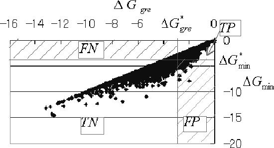
Plot of ΔG_gre versus ΔG_min for 10 000 random pairs of sequences with length 20; $\Delta G_{\text{gre}*}$ and $\Delta G_{\text{min}*}$ represent threshold of ΔG_gre and that of ΔG_min, respectively. Four terms were used for evaluating filtering performance: TP, $\left\{\left(\Delta G_{\text{gre}*}<\Delta G_{\text{gre}}\right)\wedge \left(\Delta G_{\text{min}*}<\Delta G_{\text{min}}\right)\right\}$; FN, $\left\{\left(\Delta G_{\text{gre}}\le \Delta G_{\text{gre}*}\right)\wedge \left(\Delta G_{\text{min}*}<\Delta G_{\text{min}}\right)\right\}$; FP, $\left\{\left(\Delta G_{\text{gre}*}<\Delta G_{\text{gre}}\right)\wedge \left(\Delta G_{\text{min}}\le \Delta G_{\text{min}*}\right)\right\}$; and TN, $\left\{\left(\Delta G_{\text{gre}}\le \Delta G_{\text{gre}*}\right)\wedge \left(\Delta G_{\text{min}}\le \Delta G_{\text{min}*}\right)\right\}$.

As shown in Figure 3, for FN = 0, the number of sequences classified into FP by the ΔG_gre filter was much smaller than that by the hamming filter. Because most sequences have a ΔG_min of more than −10.0 kcal/mol (Figure 2), the FP converged to zero for both the hamming filter and ΔG_gre filter for less than −10.0 kcal/mol. Similarly, for FP = 0, the number of sequences classified into FN by the ΔG_gre filter was smaller than that by the hamming filter. The reason there is little difference for greater than −5.0 kcal/mol is that a small number of sequences with the ΔG_gre actually had a ΔG_min such that $\Delta G_{\text{min}}\ll \Delta G_{\text{gre}}$. For example, sequences GGTCACCCTGGGCTACCGGA (5′ → 3′ direction) and TTAAGGTCGCGTGCTATCTT (3′ → 5′ direction) had a ΔG_min of −7.92 kcal/mol while the ΔG_gre was −1.96 kcal/mol. Because such sequences are rare, however, the primacy of the ΔG_gre filter over the hamming filter is clear for less than −5.0 kcal/mol.

Figure 3.

Threshold of ΔG_min versus number of sequences classified as FP and FN. (a) FP such that FN is zero and (b) FN such that FP is zero.

Another advantage of the ΔG_gre filter is that it guarantees having the threshold where the number of FN is zero because the ΔG_gre is the upper bound for the ΔG_min (i.e. $\Delta G_{\text{min}}\le \Delta G_{\text{gre}}$). For example, a pair of sequences having a ΔG_gre less than or equal to −5.0 kcal/mol is guaranteed to have a ΔG_min of at most −5.0 kcal/mol. Thus, the sequences with a ΔG_gre of more than −5.0 kcal/mol include all sequences with a ΔG_min of more than −5.0 kcal/mol. Therefore, setting the threshold for a ΔG_gre filter ($\Delta G_{\text{gre}}^{*}$) to that for the ΔG_min filter ($\Delta G_{\text{min}}^{*}$) (i.e. $\Delta G_{\text{gre}}^{*}=\Delta G_{\text{min}}^{*}$) guarantees that the number of FN is zero. This is not the case for hamming filter.

Comparison between hamming distance and ΔG_min in vitro

We investigated the validity of the ΔG_min based approach compared with the traditional approach based on the hamming distance by using an in vitro experiment. First, to address the validity of the ΔG_min calculation, we calculated the average deviations from the experimental free energies (ΔG_exp). The average deviations were derived from 126 sequences (31 complementary sequences, 83 sequences with a single bulge loop and 12 sequences with free ends). The average deviations, calculated using $\frac{1}{126}{\sum }_{i=1}^{126}\left|100(\Delta G_{\text{min}}^i-\Delta G_{\text{exp}}^i)\Delta /G_{\text{exp}}^i\right|$ ($\Delta G_{\text{min}}^i$ and $\Delta G_{\text{exp}}^i$ represent the i-th ΔG_min and ΔG_exp, respectively), were 3.2% (3.0, 2.8 and 6.5% for the complementary sequences, single bulges and free ends, respectively). These average deviations are within the limits of what can be expected for a nearest-neighbor model (18,19). Thus, we confirmed that our algorithm can predict the ΔG_min adequately. The 126 sequences with their ΔG_min and ΔG_exp are provided in the Supplementary Material. The number of complementary bases for each pair of sequences is also provided.

Then, to compare the hamming distance with ΔG_min, we investigated the correlation coefficient with ΔG_exp. To fairly compare different length sequences, we used the number of complementary bases but not the hamming distance. For example, although sequences 5′-GGG-3′ and 3′-CCC-5′ with three complementary bases and sequences 5′-GGGGG-3′ and 3′-CCCCC-5′ with five complementary bases both have zero hamming distance, the stability of the latter must be higher than that of the former. Thus, the number of complementary bases is appropriate for comparing the stability of sequences with different lengths. Note that the number of complementary bases is equivalent to the hamming distance for sequences with the same length. The results are shown in Figure 4a and b. In Figure 4a, BP represents the number of complementary bases. The correlation coefficient, |R|, between −BP and ΔG_exp was 0.80, while that between ΔG_min and ΔG_exp was 0.90, indicating that the ΔG_min is better than the number of complementary bases (i.e. hamming distance) as a predictor of stability.

Figure 4.

(a) −BP versus experimental free energy. BP represents the number of complementary bases. (b) Predicted minimum versus experimental free energy. In (a) and (b), values and lines are correlation coefficients and regression lines, respectively.

Bozdech et al. (5) compared the number of complementary bases with the binding energy (the calculation method and nearest-neighbor parameters differed from ours) by using 70mer oligonucleotides on microarray. They found that |R| between the binding energy and relative intensity of hybridization (= intensity of fluorescence) was 0.91, while it was 0.72 between the number of complementary bases and the relative intensity of hybridization. This is consistent with our findings, especially with respect to the correlation between the predicted energy (binding energy in theirs, ΔG_min in ours) and the stability derived from the experimental results (their |R| was 0.91, while ours was 0.90). With respect to the correlation between the number of complementary bases and the experimental stability, their |R| was 0.72, while ours was 0.80. This is because our data were derived from only sequences with a simple structure, i.e. with at most one loop (single bulge loop). In general, the more loops, the higher the discrepancy between the number of complementary bases and the experimental stability. Therefore, the correlation between the number of complementary bases and the experimental stability will be close to theirs with respect to more complex sequences, i.e. with more than two loops. These results demonstrate the ability of our program to approximate the experimental stability of double-stranded DNA based on the ΔG_min calculation.

DISCUSSION

In the previous section, we showed the effectiveness of the ΔG_gre filter for filtering out the sequences that cannot pass through the ΔG_min filter. To further address the question how the ΔG_gre is close to the ΔG_min, we investigated the average prediction error of ΔG_gre, calculated using ${\sum }_{i=1}^{10000}\left(G_{\text{gre}}^i-G_{\text{min}}^i\right)/10000$. Figure 5 shows that the average prediction error can be restricted to <1.0 kcal/mol for sequences shorter than 50mer, which are frequently used in DNA computing.

Figure 5.

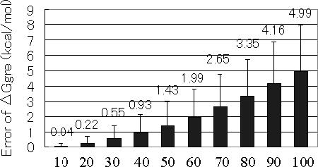
Average prediction error of ΔG_gre, calculated using ${\sum }_{i=1}^{10000}\left(\Delta G_{\text{gre}}^i-\Delta G_{min}^i\right)/10000$.

Figure 6 shows the number of sequences such that ΔG_min is equal to ΔG_gre. The number decreased as the sequences became longer. For example, $\Delta G_{\text{min}}=\Delta G_{\text{gre}}$ in 9250 pairs from 10 000 pairs of sequences at 10mer, while $\Delta G_{\text{min}}=\Delta G_{\text{gre}}$ in 157 pairs from 10 000 pairs at 100mer. Therefore, ΔG_gre is a good predictor of ΔG_min for short sequences, while it is only an approximation for long sequences.

Figure 6.

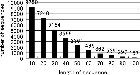
Number of sequences such that $\Delta G_{\text{min}}=\Delta G_{\text{gre}}$.

For comparison with the hamming distance, the correlation coefficient (|R|) was also calculated. The correlation between ΔG_min and ΔG_gre decreased almost linearly from 0.99 at 10mer to 0.63 at 100mer. Because long sequences tend to have more helices, the discrepancy increased as the sequences became longer. The correlation coefficient between ΔG_min and the hamming distance, which decreased almost linearly from 0.46 at 10mer to 0.12 at 100mer, was much less than that between ΔG_min and ΔG_gre.

IMPLEMENTATION

We implemented our algorithm in a program called ‘DNA Sequence Design Tool (DNA-SDT)’. DNA-SDT can be downloaded freely from the web site (http://ses3.complex.eng.hokudai.ac.jp/~fumi95/DNA-SDT/index.html). It has two functions: sequence design and structure prediction.

In sequence design, the program solves the problem of designing a pool P containing n sequences of length l for which (i) the duplex T_M is in the range $T_{\text{M}}^{-}$ to $T_{\text{M}}^{+}$ for any duplex of U_i $(0\le i\le n-1)$ and V_i and (ii) ΔG_min is greater than $\Delta G_{\text{min}}^{*}$ in any pairwise duplex of sequences in P and any concatenation of two sequences in $P\cup Q$ except for the pairwise duplex of U_i and V_i. This problem is solved using our algorithm with the threshold for a ΔG_gre filter, $\Delta G_{\text{gre}}^{*}$. The parameters, n, l, $T_{\text{M}}^{-}$, $T_{\text{M}}^{+}$, $\Delta G_{\text{gre}}^{*}$ and $\Delta G_{\text{min}}^{*}$, are user-defined. DNA-SDT has a table of average T_M values at length l $(8\le l\le 50)$ [$T_{\text{M}}^{\text{ave}}\left(l\right)$] calculated from 10 000 sequences generated randomly. Parameters $T_{\text{M}}^{-}$ and $T_{\text{M}}^{+}$ are set to $\left[T_{\text{M}}^{\text{ave}}\left(l\right)-1.5\right]$ and $\left[T_{\text{M}}^{\text{ave}}\left(l\right)+1.5\right]$, respectively, by default. The T_M is calculated at 1 μM.

In structure prediction, the program calculates the ΔG_min between two sequences, then displays the structure with the ΔG_min using a traceback algorithm. Users can thus determine the structure of any combination of sequences from the pool designed by the program. Of course, for any given combination of sequences, users can also determine the structure with the ΔG_min.

The program is a GUI-based application written in Java, hence it can be executed on any computer that has the Java Runtime Environment (JRE) installed. Although older versions of JRE supposedly run without problem, the latest version is preferable. We tested the program with JRE 1.4.2 on a Windows 2000 workstation, JRE 1.4.1 on a Windows XP workstation and JRE 1.4.2 on a Turbolinux Workstation 7.0.

The program interface consists of two screens: one for structure prediction and one for sequence design. The left-hand side of the window is the screen for structure prediction, which outputs the structure with the ΔG_min from the two sequences input in the text box. The sequences in the text box can be converted into reverse or complementary sequences. The right-hand side is the screen for sequence design, which outputs the sequences, GC content and T_M based on the constraints input in the text boxes.

To avoid impossible operations during design, the procedure for sequence design is executed as a separate thread. Therefore, the structure-prediction screen can be operated freely when sequences are being designed. Furthermore, the design procedure can be monitored and interrupted anytime, and the interim results can be output. However, because the button for running the sequence design procedure is locked during design, users cannot design another pool of sequences in parallel.

The number of sequences can be set up to 100. If more than 100 sequences need to be designed, the user can choose ‘Unlimited’. In this case, the design procedure iterates until the user interrupts it. The sequence length is restricted at 8mer to 50mer because of the computation time. Although the thresholds for ΔG_min and ΔG_gre can be set freely, using irrelevant values resulting in zero sequences. We recommend setting these thresholds such that $\Delta G_{\text{min}}^{*}=\Delta G_{\text{gre}}^{*}(<0)$ to guarantee zero false negatives (see Results).

SUPPLEMENTARY MATERIAL

Supplementary Material is available at NAR Online.

REFERENCES

- 1.Adleman L.M. Molecular computation of solutions to combinatorial problems. Science. 1994;266:1021–1024. doi: 10.1126/science.7973651. [DOI] [PubMed] [Google Scholar]
- 2.Braich R.S., Chelyapov N., Johnson C., Rothemund P.W., Adleman L. Solution of a 20-variable 3-SAT problem on a DNA computer. Science. 2002;296:499–502. doi: 10.1126/science.1069528. [DOI] [PubMed] [Google Scholar]
- 3.Faulhammer D., Cukras A.R., Lipton R.J., Landweber L.F. Molecular computation: RNA solutions to chess problems. Proc. Natl Acad. Sci. USA. 2000;97:1385–1389. doi: 10.1073/pnas.97.4.1385. [DOI] [PMC free article] [PubMed] [Google Scholar]
- 4.Rouillard J.M., Zuker M., Gulari E. OligoArray 2.0: design of oligonucleotide probes for DNA microarrays using a thermodynamic approach. Nucleic Acids Res. 2003;31:3057–3062. doi: 10.1093/nar/gkg426. [DOI] [PMC free article] [PubMed] [Google Scholar]
- 5.Bozdech Z., Zhu J., Joachimiak M.P., Cohen F.E., Pulliam B., DeRisi J.L. Expression profiling of the schizont and trophozoite stages of Plasmodium falciparum with a long-oligonucleotide microarray. Genome Biol. 2003;4:R9. doi: 10.1186/gb-2003-4-2-r9. [DOI] [PMC free article] [PubMed] [Google Scholar]
- 6.Kane M.D., Jatkoe T.A., Stumpf C.R., Lu J., Thomas J.D., Madore S.J. Assessment of the sensitivity and specificity of oligonucleotide (50mer) microarrays. Nucleic Acids Res. 2000;28:4552–4557. doi: 10.1093/nar/28.22.4552. [DOI] [PMC free article] [PubMed] [Google Scholar]
- 7.Winfree E., Liu F., Wenzler L.A., Seeman N.C. Design and self-assembly of two-dimensional DNA crystals. Nature. 1998;394:539–544. doi: 10.1038/28998. [DOI] [PubMed] [Google Scholar]
- 8.Shih W.M., Quispe J.D., Joyce G.F. A 1.7-kilobase single-stranded DNA that folds into a nanoscale octahedron. Nature. 2004;427:618–621. doi: 10.1038/nature02307. [DOI] [PubMed] [Google Scholar]
- 9.Yan H., Zhang X., Shen Z., Seeman N.C. A robust DNA mechanical device controlled by hybridization topology. Nature. 2002;415:62–65. doi: 10.1038/415062a. [DOI] [PubMed] [Google Scholar]
- 10.Arita M., Kobayashi S. DNA sequence design using templates. New Gen. Comput. 2002;20:263–277. [Google Scholar]
- 11.Arita M., Nishikawa A., Hagiya M., Komiya K., Gouzu H., Sakamoto K. Improving sequence design for DNA computing. In Proceedings of the Genetic and Evolutionary Computation Conference (GECCO-2000); 2000. pp. 875–882. [Google Scholar]
- 12.Dirks R.M., Lin M., Winfree E., Pierce N.A. Paradigms for computational nucleic acid design. Nucleic Acids Res. 2004;32:1392–1403. doi: 10.1093/nar/gkh291. [DOI] [PMC free article] [PubMed] [Google Scholar]
- 13.Andronescu M., Fejes A.P., Hutter F., Hoos H.H., Condon A. A new algorithm for RNA secondary structure design. J. Mol. Biol. 2004;336:607–624. doi: 10.1016/j.jmb.2003.12.041. [DOI] [PubMed] [Google Scholar]
- 14.Andronescu M., Aguirre-Hernandez R., Condon A., Hoos H.H. RNAsoft: a suite of RNA secondary structure prediction and design software tools. Nucleic Acids Res. 2003;31:3416–3422. doi: 10.1093/nar/gkg612. [DOI] [PMC free article] [PubMed] [Google Scholar]
- 15.Hofacker I.L. Vienna RNA secondary structure server. Nucleic Acids Res. 2003;31:3429–3431. doi: 10.1093/nar/gkg599. [DOI] [PMC free article] [PubMed] [Google Scholar]
- 16.Mathews D.H., Sabina J., Zuker M., Turner D.H. Expanded sequence dependence of thermodynamic parameters improves prediction of RNA secondary structure. J. Mol. Biol. 1999;288:911–940. doi: 10.1006/jmbi.1999.2700. [DOI] [PubMed] [Google Scholar]
- 17.Zuker M., Stiegler P. Optimal computer folding of large RNA sequences using thermodynamics and auxiliary information. Nucleic Acids Res. 1981;9:133–148. doi: 10.1093/nar/9.1.133. [DOI] [PMC free article] [PubMed] [Google Scholar]
- 18.SantaLucia J., Jr A unified view of polymer, dumbbell, and oligonucleotide DNA nearest-neighbor thermodynamics. Proc. Natl Acad. Sci. USA. 1998;95:1460–1465. doi: 10.1073/pnas.95.4.1460. [DOI] [PMC free article] [PubMed] [Google Scholar]
- 19.Tanaka F., Kameda A., Yamamoto M., Ohuchi A. Thermodynamic parameters based on a nearest-neighbor model for DNA sequences with a single-bulge loop. Biochemistry. 2004;43:7143–7150. doi: 10.1021/bi036188r. [DOI] [PubMed] [Google Scholar]
- 20.Zuker M. Mfold web server for nucleic acid folding and hybridization prediction. Nucleic Acids Res. 2003;31:3406–3415. doi: 10.1093/nar/gkg595. [DOI] [PMC free article] [PubMed] [Google Scholar]
- 21.Peritz A.E., Kierzek R., Sugimoto N., Turner D.H. Thermodynamic study of internal loops in oligoribonucleotides: symmetric loops are more stable than asymmetric loops. Biochemistry. 1991;30:6428–6436. doi: 10.1021/bi00240a013. [DOI] [PubMed] [Google Scholar]
- 22.Bommarito S., Peyret N., SantaLucia J., Jr Thermodynamic parameters for DNA sequences with dangling ends. Nucleic Acids Res. 2000;28:1929–1934. doi: 10.1093/nar/28.9.1929. [DOI] [PMC free article] [PubMed] [Google Scholar]
- 23.Lyngsø R.B., Zuker M., Pedersen C.N.S. Fast evaluation of internal loops in RNA secondary structure prediction. Bioinformatics. 1999;15:440–445. doi: 10.1093/bioinformatics/15.6.440. [DOI] [PubMed] [Google Scholar]
Associated Data
This section collects any data citations, data availability statements, or supplementary materials included in this article.