The Generalized Higher Criticism for Testing SNP-Set Effects in Genetic Association Studies

Abstract

It is of substantial interest to study the effects of genes, genetic pathways, and networks on the risk of complex diseases. These genetic constructs each contain multiple SNPs, which are often correlated and function jointly, and might be large in number. However, only a sparse subset of SNPs in a genetic construct is generally associated with the disease of interest. In this article, we propose the generalized higher criticism (GHC) to test for the association between an SNP set and a disease outcome. The higher criticism is a test traditionally used in high-dimensional signal detection settings when marginal test statistics are independent and the number of parameters is very large. However, these assumptions do not always hold in genetic association studies, due to linkage disequilibrium among SNPs and the finite number of SNPs in an SNP set in each genetic construct. The proposed GHC overcomes the limitations of the higher criticism by allowing for arbitrary correlation structures among the SNPs in an SNP-set, while performing accurate analytic p-value calculations for any finite number of SNPs in the SNP-set. We obtain the detection boundary of the GHC test. We compared empirically using simulations the power of the GHC method with existing SNP-set tests over a range of genetic regions with varied correlation structures and signal sparsity. We apply the proposed methods to analyze the CGEM breast cancer genome-wide association study. Supplementary materials for this article are available online.

1. Introduction

With the abundance of genome-wide association studies (GWAS) and with the increase in large-scale sequencing studies, there is an increasing demand for development of advanced methodology capable of improving our chance for detecting genetic associations for complex diseases and traits. Common analysis of GWAS data tests single nucleotide polymorphisms (SNPs) individually (Manolio et al. 2009; Visscher et al. 2012). GWAS has been successful in identifying thousands of SNPs associated with complex diseases and traits. However, it has been shown that individual SNP effects are generally weak, and the disease/trait associated SNPs identified in GWAS are insufficient in explaining much of the heritability of complex diseases and traits, even for highly heritable traits, such as height (Visscher et al. 2012).

These findings suggest that single SNP analysis may be underpowered. This is particularly the case for low-frequency SNPs in sequencing association studies (Lee et al. 2014). Region-based analyses have recently become more popular in genetic association studies as a complementary approach to individual SNP analysis by combining information from multiple SNPs in a genetic construct (Li and Leal 2008; Lee et al. 2014). Genes, gene networks, and pathways are examples of genetic constructs that are likely to have multiple SNPs that function simultaneously to affect diseases and traits, for example, due to functional similarity or interaction. The signal SNPs in a genetic construct are likely to be sparse and have weak signals. Hence, a methodology that does not require strong marginal SNP effects but is capable of aggregating these weak and sparse SNP effects together into a detectable signal at the genetic construct level, such as a gene, is needed to help increase the chance of detecting the effects of these genetic constructs and find the causes of the missing heritability.

Motivating data examples are the data from the Cancer Genetic Markers of Susceptibility (CGEM) GWAS breast cancer study, which is a case-control study with postmenopausal women of European ancestry that was aimed at identifying genetic variants that are associated with breast cancer risk (Hunter et al. 2007). These authors analyzed the data by examining the effects of individual SNPs across the genome. They found that several SNPs in the FGFR2 region showed strong evidence of association with breast cancer risk using individual SNP analysis. These results were validated in a separate study sample. However, none of these SNPs reached genome-wide significance when analyzing the CGEM GWAS data using the traditional individual SNP analysis.

In an effort to gain more power by studying genetic constructs (SNP sets), for example, genes, instead of individual SNPs, Wu et al. (2010) scanned the genome at the gene level and found the FGFR2 region to be more significantly associated with breast cancer. Though the region contained 35 SNPs, the signal was sparse with only four of the SNPs showing evidence of any association with disease. Indeed, marginally, none of those four SNPs were at genome-wide significance levels due to the large multiple testing problem. However, when the signals from all SNPs in the region were treated as a unit, then the association became more significant. The approach of Wu et al. (2010) equally uses all the SNPs in FGFR2 and does not take into account the fact that the signals are sparse in this region. It is hence of substantial interest to develop a test that can be more powerful in the presence of sparse signals.

Sparse signals in an SNP set, present a particularly difficult problem for detection. As will be shown, the current methodology for SNP-set testing excels when signals are dense and prevalent, but is greatly affected by loss of power when sparsity is high. Given this, the likely existence of undiscovered disease-associated genes and other SNP-sets requires new methodology that is better capable of detecting sparse signals. In addition, due to their close proximity, it is common for SNPs within the same gene to be correlated, also known as being in linkage disequilibrium (LD). As an example, Figure 1 shows the LD map of the FGFR2 gene region, which demonstrates that some SNPs in this region are in high and moderate LD. This demonstrates the importance of having a methodology for testing SNP-sets that is powerful when the signal is sparse while also accounting for the LD between SNPs.

Figure 1.

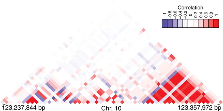
The LD plot of the FGFR2 gene based on the CGEM genetic association study of breast cancer data. Pearson correlations are displayed, with negative correlations in blue and positive correlations in red.

Several methods have been proposed for SNP-set testing, such as MinP and variance-component tests. MinP calculates the marginal test statistic for each SNP in an SNP-set and then uses the maximum (or most extreme) marginal test statistic as the representative test statistic while adjusting for correlation among the test statistics within the SNP-set (Conneely and Boehnke 2007; Moskvina and Schmidt 2008; Zhang and Liu 2011). MinP has low power when multiple SNPs do not have strong signals and instead combine together to form a strong signal. Variance-component tests such as the Sequence Kernel Association Test (SKAT) offer an alternative to MinP for detecting SNP-set associations by combining all SNP information over the SNP-set (Wu et al. 2010; Chen, Meigs, and Dupuis 2013; Ionita-Laza et al. 2013). However, it equally aggregates information across all the SNPs and does not take into account that signals might be sparse. Hence, if the signal in the region is sparse, then SKAT can have low power due to giving equal weight to noncausal SNPs in the region, which can cover up the signal with noise.

The higher criticism is a global test that combines information over all the marginal test statistics of a set of variables (Donoho and Jin 2004). It provides an attractive approach for testing for the effect of an SNP set by combining information across a sparse few disease-associated SNPs out of a large pool of unassociated SNPs if the SNPs were independent or sparsely and weakly correlated (Arias-Castro, Candès, and Plan 2011). Wu et al. (2014) studied the asymptotic power of the higher criticism of Donoho and Jin (2004) and showed its value in the sparse signal regime for testing the effect of an SNP-set in genetic association studies. These results rely on asymptotic p-values and assume the SNPs to be independent or sparsely weak correlated (Arias-Castro, Candès, and Plan 2011), which generally do not hold in GWAS.

There are several limitations of directly applying the higher criticism to testing for the SNP set effect in GWAS. First, some SNPs in an SNP set are strongly correlated due to LD. Second, the asymptotics of the higher criticism requires the number of SNPs (p) in a genetic construct to be extremely large, for example, p > 10⁶. However, the number of SNPs in a genetic construct is finite and not very large. For example, p is usually in tens to thousands in a gene and in hundreds to thousands in a genetic pathway or a network. Hence, these implementations of the higher criticism based on asymptotic results give quite biased p-values in practice (Barnett and Lin 2014), and one often has to rely on simulations to calculate p-values more accurately for testing for genetic constructs. However, these simulation-based p-value calculations for genes are computationally unpractical when used to scan the genome at the gene-level in GWAS. Recently, methods for obtaining accurate p-values of the higher criticism analytically for any finite number of SNPs in a SNP set have been developed for the case when test statistics are independent (Barnett and Lin 2014; Moscovich-Eiger, Nadler, and Spiegelman 2013). However, these methods are not directly applicable to GWAS and will yield biased p-values as SNPs in a genetic construct are commonly correlated due to LD.

To handle an arbitrary correlation structure among individual tests in a global test of a set of variables, Hall and Jin (2010) proposed the innovated higher criticism (iHC), which first transforms the test statistics to independent test statistics using the Cholesky decomposition of the correlation matrix and then applies the higher criticism after the transformation. We will show that iHC based on this transformation can be unstable when SNPs are in high LD, and is also subject to considerable loss of power in the presence of correlation among the SNPs, as shown in our numerical studies.

In this article, we propose the generalized higher criticism (GHC) test statistic that is suitable for testing for the effect of an SNP-set in GWAS containing any finite number of correlated SNP markers. The GHC method accounts for sparse signals and the correlation among the SNPs in both the construction of the test statistic and analytic p-value calculations. It does not require any transformation of the original test statistics. In contrast to prior treatments of the higher criticism, the GHC is both flexible to any correlation structure while obtaining its analytic p-values in an accurate and computationally efficient manner without requiring simulation of the null distribution. Hence, it is computationally feasible and accurate when scanning the whole genome in GWAS by adapting to varying LD structures in different genes. We also studied the asymptotic properties of GHC.

The power of GHC relative to iHC, SKAT, and MinP is compared over extensive simulations using SNP-sets with varied correlation structures by generating genotype data similar to GWAS. While MinP and SKAT are sensitive to sparsity, the robustness of GHC is demonstrated through simulation over regions with varying degrees of sparsity and LD structures. With a wide variety of LD patterns across the genome, it is not only important for a test to be robust to signal sparsity, but a reliable test must also be robust to a wide range of correlation structures. Many tests, such as SKAT, can lose power if a strong LD block in an SNP-set does not contain the causal SNPs. The GHC avoids this problem by thresholding the marginal test statistics. As a result, its power is robust to the correlation structure. We show in some situations SKAT and MinP can be more powerful than GHC. Hence, to increase the power for detecting the effects of genes across the genome that have a wide range of sparsity and correlation structures, we also propose the omnibus test by combining the GHC, MinP, and SKAT, and show it is robust and powerful.

We applied the GHC to perform a gene-based genome-wide analysis of the GWAS data of the Cancer Genetic Markers of Susceptibility breast cancer study. We compared the performance of GHC with the competing methods for their ability to detect the genetic associations with breast cancer risk across the full spectrum of correlation structures and sparsity levels that the genome has to offer. In addition to p-value comparison, the Type I error rates for GHC are shown to be accurate in both high LD and low LD SNP-sets, as well as through simulations across a wide range of randomly selected genes taken from the CGEM data.

The remainder of the article is organized as follows. In Section 2, we introduce the SNP-set generalized linear model. In Section 3, we briefly review the higher criticism as well as the problems it has in accounting for correlation among SNPs in SNP-sets. In Section 4, we propose the GHC and an analytic accurate procedure for obtaining p-values using the GHC for any arbitrary correlation structure and size of a SNP set. In Section 5, some results of the asymptotic detection boundary for GHC are established. In Section 6, the omnibus test combining SKAT, MinP, and GHC is introduced. In Section 7, we evaluate the performance of the GHC relative to competing methods using extensive simulations. In Section 8, the GHC and competing methods are used to analyze the CGEM breast cancer GWAS data. Finally, we conclude with discussions in Section 9.

2. Generalized Linear Model and Marginal SNP Score Test Statistics

We consider a sample of N individuals genotyped over a region with p observed SNPs in a SNP-set. Possible SNP-sets include genes, gene networks, or genetic pathways. Individuals have phenotypes Y = [Y₁, …,Y_N]^T. The N by p genotype matrix G is constructed such that G_i = [G_i1, …, G_ip]^T with ${\mathit{G}}_i^T$ as the ith row vector of G containing the genotypes in a genetic construct for the ith individual. The N by q matrix X contains covariates, with X_i = [X_i1, …, X_iq]^T and ${\mathit{X}}_{\mathit{i}}^T$ being the ith row vector of X containing the covariate values for the ith individual. Suppose that conditional on (X_i, G_i), Y_i follows a distribution in the exponential family (MacCullagh and Nelder 1989) f (Y_i) =exp{(Y_iθ_i − b(θ_i))/a_i(ϕ) + c(Y_i, ϕ)}, where f (Y_i) is the conditional distribution of Y_i|(X_i, G_i), a(·), b(·), and c(·) are known functions, θ_i is the canonical parameter, and ϕ is the dispersion parameter. To construct a marginal test between the jth SNP and Y, we model μ_i = E(Y_i|G_i, X_i) = b^′(θ_i) using the generalized linear model (GLM) (MacCullagh and Nelder 1989)

$$g\left({\mu }_i\right)={\mathit{X}}_{\mathit{i}}^T\mathit{\alpha }+{\mathit{G}}_{\mathit{i}}^T\mathit{\beta },$$ (1)

where g(·) is a link function and (α, β) are the regression coefficients. For simplicity, we here restrict to the canonical link. The variance of Y_i is Var(Y_i) = a_i(ϕ)v(μ_i), where v(μ_i) = b^″(θ_i) is a variance function. The dispersion parameter ϕ is replaced by its estimate for normally distributed outcomes but needs not be estimated for dichotomous outcomes. We are interested in testing for the overall effect of the SNP set G_i, which corresponds to the global null H₀ : β = 0.

The dimension p of β might be large. In a genetic construct, SNPs are often correlated and generally only a small subset of SNPs are signals, that is, a sparse set of the β_j are not zero. The proposed GHC test aims at accounting for both sparse signals and correlation among SNPs when combining individual marker test statistics.

Letting $\mathit{W}=\text{diag}\{a_1(\widehat{\varphi })\upsilon ({\widehat{\mu }}_{01}),\dots ,a_n(\widehat{\varphi })\upsilon ({\widehat{\mu }}_{0n})\}$ and P = W − WX(X^TWX)⁻¹X^TW, the marginal score test statistic for β_j under the global null is

$$Z_j=\frac{{\mathit{G}}_{\mathit{j}}^T(\mathit{Y}-{\widehat{\mathit{\mu }}}_0)}{\sqrt{{\mathit{G}}_{\mathit{j}}^T\mathit{P}{\mathit{G}}_{\mathit{j}}}},$$ (2)

where ${\widehat{\mathit{\mu }}}_0=\mathit{\mu }\left(\mathit{X}\widehat{\mathit{\mu }}\right),\widehat{\mathit{\alpha }}$ is the MLE of α under the null model of $g\left({\mu }_i\right)={\mathit{X}}_{\mathit{i}}^T\mathit{\alpha }$, and G_j denotes the jth column vector of G. These individual SNP test statistics are asymptotically jointly distributed as $\mathit{Z}~\text{MVN}\left(\mathbf{0},\sum \right)$, where we estimate cov(Z_j, Z_k) = σ_jk, the (j, k)th component of Σ by

$${\widehat{\sigma }}_{jk}=\frac{{\mathit{G}}_{\mathit{j}}^T\mathit{P}{\mathit{G}}_{\mathit{k}}}{\sqrt{{\mathit{G}}_{\mathit{j}}^T\mathit{P}{\mathit{G}}_j}\sqrt{{\mathit{G}}_{\mathit{k}}^T\mathit{P}{\mathit{G}}_{\mathit{k}}}}.$$

While the Z are correlated, we define the uncorrelated transformed test statistics Z^∗ to be

$$\mathit{Z}\ast ={\mathit{U}}^{-1}\mathit{Z}~\mathit{MVN}\left(\mathbf{0},{\mathit{I}}_p\right),$$

where $\mathit{U}{\mathit{U}}^T=\widehat{\mathbf{\sum }}$ is the Cholesky decomposition.

3. The Higher Criticism Test

The higher criticism tests H₀ : β = 0 from model (1) against the alternative that a sparse set of the β_j are nonzero. An idea proposed first in passing by Tukey, the higher criticism was developed by Donoho and Jin (2004) for summary statistics in the setting where under the alternative the marginal test statistics come from a mixture of normal random variables, as well as by Arias-Castro, Candès, and Plan (2011) in the regression setting. Because the Z are correlated, Hall and Jin (2010) proposed a higher criticism test based on the transformed Z^∗. To do so, let

$$S\ast \left(t\right)={\displaystyle \sum _{j=1}^p{\mathbf{1}}_{\left\{|Z_j^{\ast }|\ge t\right\}}.}$$

Note that under H₀, S^∗(t) ∼ Binomial $\left(p,2\overline{\mathrm{\Phi }}\left(t\right)\right)$, where $2\overline{\mathrm{\Phi }}\left(t\right)=1-\mathrm{\Phi }\left(t\right)$ is the survival function of the normal distribution. The innovated Higher Criticism (iHC) test statistic is defined as

$$\mathit{iHC}={\sup }_{t\ge t_0}\left\{\frac{S\ast \left(t\right)-2p\overline{\mathrm{\Phi }}\left(t\right)}{\sqrt{2p\overline{\mathrm{\Phi }}\left(t\right)\left(1-2\overline{\mathrm{\Phi }}\left(t\right)\right)}}\right\}$$

for some t₀ ≥ 0. This test rejects H₀ for large values of iHC.

There are drawbacks to iHC due to having to first transform the marginal test statistics from Z into Z^∗. In the presence of even moderately small correlation, there can be a significant loss of power due to the noise diluting the sparse signals after being mixed in the transformation. For example, alleles in the FGFR2 gene have been linked to breast cancer risk (Hunter et al. 2007). The CGEM breast cancer data has 35 SNPs in the gene, four of which have marginal test statistics greater than 4.3 in absolute value indicating a strong association between FGFR2 and breast cancer incidence. However, after transforming these test statistics to become Z^∗, none of the transformed statistics exceed 2.6 in absolute value (Figure 2). These transformed test statistics are so attenuated toward the null that it can lead to a significant loss in power. This motivates our generalization of the higher criticism to accommodate the use of the original untransformed correlated test statistics Z to avoid this loss of power.

Figure 2.

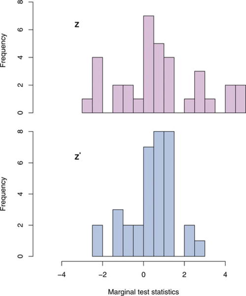
The marginal test statistics for 35 SNPs from the FGFR2 gene, each with MAF > 0.05, from the CGEM genetic association study of breast cancer are plotted. The original test statistics Z are in the top histogram, while the transformed test statistics Z^∗ = U⁻¹Z are in the bottom histogram.

If we allow p → ∞, the higher criticism has been shown to be powerful for high sparsity situations (i.e., when the number of β_j ≠ 0 are less than $\sqrt{p}$) with low dependence (Donoho and Jin 2004; Hall and Jin 2010). For very large p, iHC can be viewed as the supremum of a normalized empirical process which converges asymptotically to a Gumbel distribution at a very slow rate of O{(log p)^−1/2} (Jaeschke 1979). With such a slow rate of convergence, the size of the test is drastically incorrect when using the asymptotic distribution to calculate p-values for p as large as a million (Barnett and Lin 2014). Around 92% of genes in GWAS have p < 50, and with most functional networks and pathways containing a few hundred genes, the size of SNP-sets in both gene-level and pathway-level analyses are generally not large enough for the asymptotic distribution of the iHC to be of any practical use.

For finite p, a different analytic approach to finding the distribution of the iHC statistic must be taken. As the transformed test statistics Z^∗ used in iHC are independent, the exact p-value calculation that was developed for the original higher criticism for independent marginal test statistics (Barnett and Lin 2014) can be used for p-value calculation for iHC without relying on asymptotics. This p-value calculation is an exact and computationally efficient method for all finite p, and therefore ideal for testing SNP-sets in genetic association studies. We build on this approach to further accomodate correlation to avoid the power loss that results from using the decorrelated Z^∗.

4. The Generalized Higher Criticism Test

If the LD structure in a gene or SNP-set is even moderately weak, it is likely that transforming Z by U⁻¹ can result in the transformed test statistics Z^∗ being underpowered. In addition, for stronger LD, which is common between some SNPs, the matrix inverse operation of U⁻¹ can be quite unstable. To avoid the drawbacks of such a transformation, we propose the generalized higher criticism (GHC) test statistic based on the original Z.

4.1. Definition of the Generalized Higher Criticism (GHC) Test

Define S(t) as

$$S\left(t\right)={\displaystyle \sum _{j=1}^p{\mathbf{1}}_{\left\{\left|Z_j\right|\ge t\right\}}.}$$

For general Σ ≠ I_p, S(t) is no longer binomial. The correlation among the SNPs in a SNP set, whether positive or negative, increases the variance. Using the original higher criticism in this case would result in standardizing with the incorrect variance. Furthermore, analytic p-value calculations of the original higher criticism using Barnett and Lin (2014) when applied to the original Z statistics, fail to account for the correlation among the original Z statistics, and will hence result in biased p-values and incorrect Type I error rates. Instead, we estimate cov(S(t_j), S(t_k)) using the sample correlation $\widehat{\mathbf{\sum }}$ using Theorem 1, and account for the correlation among the marginal Z statistics when deriving the distribution of the proposed generalized higher criticism (GHC).

Theorem 1

Let $\overline{r^n}=\frac{2}{p\left(p-1\right)}{{\displaystyle {\sum }_{1\le k<l\le p}\left({\sum }_{kl}\right)}}^n$ and let ${\mathscr{H}}_i\left(t\right)$ be the Hermite polynomials: ${\mathscr{H}}_0\left(t\right)=1,{\mathscr{H}}_1\left(t\right)=t,{\mathscr{H}}_2\left(t\right)=t^2-1$, and so on. Then

$$\begin{array}{c}\text{cov}\left\{S\left(t_k\right)\right\}=p\left[2\overline{\mathrm{\Phi }}(max\{t_j,t_k\}\right)-4\overline{\mathrm{\Phi }}\left(t_j\right)\overline{\mathrm{\Phi }}\left(t_k\right)]\\ +4p\left(p-1\right)\varphi \left(t_j\right)\varphi \left(t_k\right)\\ \times {\displaystyle \sum _{i=1}^{\infty }\frac{{\mathscr{H}}_{2i-1}\left(t_j\right){\mathscr{H}}_{2i-1}\left(t_k\right)\overline{r^{2i}}}{\left(2i\right)!}}.\end{array}$$

The proof of Theorem 1 is left to the supplementary materials. Using Theorem 1 with $\widehat{\mathbf{\sum }}$ instead of Σ we obtain estimates of var(S(t)). Though Theorem 1 involves an infinite sum, the terms tend to zero so rapidly that in practice we suggest that only the first few terms are necessary for estimating the covariance with great accuracy. For example, in simulation studies, we have found first eight terms will provide sufficient accuracy. With these estimates, we define the generalized higher criticism test statistic to be:

$$\text{GHC}=\underset{t\ge t_0}{\sup }\left\{\frac{S\left(t\right)-p\cdot 2\overline{\mathrm{\Phi }}\left(t\right)}{\sqrt{\widehat{\mathrm{var}}\left(S\left(t\right)\right)}}\right\}.$$ (3)

For simplicity, we will assume t₀ = 0. In the independent case when $\widehat{\mathbf{\sum }}={\mathit{I}}_p$, the GHC statistic reduces to the original higher criticism. The stronger the correlation structure, the larger the denominator (3) becomes. However the GHC numerator tends to be larger than the iHC numerator due to the transformed Z^∗ being attenuated toward the null. If the Z_j’s were normally distributed and Σ_jk = 0 for $\left|j-k\right|>b$ for some fixed bandwidth b, which usually holds in GW|AS, then as N, p → ∞, Hoeffding and Robbins (1948) show using the central limit theorem for dependent random variables that $\left(S\left(t\right)-p\cdot 2\overline{\mathrm{\Phi }}\left(t\right)\right){\left(\widehat{\mathit{Var}}\left(S\left(t\right)\right)\right)}^{-1/2}$ converges to the standard normal distribution.

Convergence of the GHC under the null can be established under suitable mixing conditions (Doukhan 1991) following ideas from Andrews and Pollard (1994) and Leadbetter, Lindgren, and Rootzén (1983). Refer to Zhong et al. (2013) for more details. In Section 5, we establish the asymptotic minimax detection boundary for GHC under weak correlation conditions similar to Arias-Castro, Candès, and Plan (2011) for Gaussian outcomes. Since mixing conditions do not necessarily translate into weak correlation conditions, we do not pursue establishing the asymptotic null distribution of GHC under mixing conditions. However, it is worth noting, that the slow convergence to the asymptotic null distribution of iHC is present for GHC as well, under suitable mixing conditions.

Parallel to the results of the higher criticism (Barnett and Lin 2014), the asymptotic distribution of GHC requires an extremely large p for the approximation to work. As the number of SNPs in a genetic construct is finite and is not extremely large, asymptotic-based p-value calculations of GHC are not accurate in genetic association studies. Hence, in the next section, we propose a more accurate p-value calculation for GHC in finite p settings that does not rely on asymptotics.

4.2. Calculation of the Generalized Higher Criticism p-value for Finite p

For a given observed GHC statistic, h, we show in the supplementary materials that the corresponding p-value is

$$\text{pr}\left(\text{GHC}\ge h\right)=1-{\displaystyle \prod _{k=1}^p{\displaystyle \sum _{a=0}^{p-k}{q}_{k,a},}}$$ (4)

where, for k > 1,

$$\begin{array}{l}{q}_{k,a}={\displaystyle \sum _{m=0}^{p-k+1}\text{pr}\left(S\left(t_k\right)=a|S\left(t_{k-1}\right)=m,{\displaystyle \underset{l=1}{\overset{k-2}{\cap }}\left\{S\left(t_l\right)\le p-l\right\}}\right)}\\ \times \frac{q_{k-1,m}}{{\displaystyle {\sum }_{l=0}^{p-k+1}qk-1,l}},\end{array}$$

for k = 1, q_1,a = pr(S(t₁) = a), and t_k is solved for in the equation

$$h\sqrt{\widehat{\mathrm{var}}\left(S\left(t_k\right)\right)}+2p\overline{\mathrm{\Phi }}\left(t_k\right)=p-k+1$$ (5)

for each k ∈ {1, …, p.

When the test statistics are independent Σ= I_p, then S(t) is the sum of independent indicator variables and the distribution of S(t_k) conditional on S(k_t−1) = m and ${\displaystyle {\cap }_{l=1}^{k-2}\left\{S\left(t_l\right)\le p-l\right\}}$ is binomial with m events and probability of success $\overline{\mathrm{\Phi }}\left(t_k\right)/\overline{\mathrm{\Phi }}\left(t_{k-1}\right)$. When calculating the p-value for GHC for general Σ, S(t) is not binomially distributed. Since S(t) is a sum of correlated binary random variables, S(t) follows an overdispersed binomial distribution (MacCullagh and Nelder 1989). Hence, to account for overdispersion, the distribution of S(t_k) conditional on S(t_{k − 1}) = m and ${\displaystyle {\cap }_{l=1}^{k-2}\left\{S\left(t_l\right)\le p-l\right\}}$ is approximated with a beta-binomial distribution (Crowder 1978).

The condition distribution of S(t_k) is approximated by

$$\begin{array}{l}\text{pr}\left(S\left(t_k\right)=a|S\left(t_{k-1}\right)=m,{\displaystyle \underset{l=1}{\overset{k-2}{\cap }}\left\{S\left(t_l\right)\le p-l\right\}}\right)\\ \approx \text{pr}\left(S\left(t_k\right)=a|S\left(t_{k-1}\right)=m\right).\end{array}$$

This approximation is an equality if the marginal test statistics are independent due to the Markov property of empirical processes (Gaenssler 1983). The approximation accuracy decreases as correlation increases, and we show in through a simulation study that this approximation works well in practice when analyzing GWAS data. The variance of S(t_k) conditional on S(t_k−1) = m is obtained by conditioning on which of the m different |Z_j| are greater than t_k−1. The expectation is $m\cdot \overline{\mathrm{\Phi }}\left(t_k\right)/\overline{\mathrm{\Phi }}\left(t_{k-1}\right)$ just like in the independent case. Using these first two moments, the parameters of the beta-binomial distribution (α and β) are solved for numerically using moment matching in the equations

$$\begin{array}{l}m\frac{\overline{\mathrm{\Phi }}\left(t_k\right)}{\overline{\mathrm{\Phi }}\left(t_{k-1}\right)}=\frac{m\alpha }{\alpha +\beta },2\frac{\left(\begin{array}{c}m\\ 2\end{array}\right)}{\left(\begin{array}{c}p\\ 2\end{array}\right)}{\displaystyle \sum _{j<l}\frac{\text{pr}\left(\left|Z_j\right|,\left|Z_l\right|>t_k\right)}{\text{pr}\left(\left|Z_j\right|,\left|Z_l\right|>t_{k-1}\right)}}\\ +m\frac{\overline{\mathrm{\Phi }}\left(t_k\right)}{\overline{\mathrm{\Phi }}\left(t_{k-1}\right)}-{\left(m\frac{\overline{\mathrm{\Phi }}\left(t_k\right)}{\overline{\mathrm{\Phi }}\left(t_{k-1}\right)}\right)}^2\\ =\frac{m\alpha \beta \left(\alpha +\beta +m\right)}{{\left(\alpha +\beta \right)}^2\left(\alpha +\beta +1\right)},\end{array}$$

where pr(|Z_j|, |Z_l| > t_k) can be obtained as in Schwartzman and Lin 2011) (see the supplementary materials). The unconditional distribution of S(t_k) can be obtained in the same way by substituting t_k−1 = 0 and m = p.

5. The Detection Boundary of GHC

In this section, we examine the asymptotic properties of GHC with hopes that its asymptotic properties can help inform us about the performance of GHC in a more general setting. Asymptotic results, in particular, the detection boundary, for the higher criticism have been well studied in the context of Gaussian linear regression for low-coherence design matrices (Arias-Castro, Candès, and Plan 2011). The detection boundary refers to a function of sparsity that defines the minimum signal strength required for a test to be asymptotically powerful (Ingster, Tsybakov, and Verzelen 2010). Recall that, from Equation (2) we have that the score vector Z is approximately multivariate normal in large samples. Hence, it is worth exploring, if the proposed GHC test attains the detection boundaries obtained in Arias-Castro, Candès, and Plan (2011) and Ingster, Tsybakov, and Verzelen (2010) under the same regularity conditions for linear regression of normally distributed outcomes. Since in large samples, the Z-statistic approaches a multivariate normal distribution, this is likely to provide one intuition with validity of the proposed method in an asymptotic sense under suitable regularity conditions. Indeed, the degree of closeness to a normal experiment in some sense, is crucial to decide sharp detection limits for the problem in a GLM.

For a general class of design matrices and in the GLM framework, it is a subtle problem and does not follow directly from the Gaussian linear regression results. In particular, Mukherjee, Pillai, and Lin (2015) demonstrated that for binary regression models under certain sparsity structures on discrete design matrices, there exists an extra phase transition for the detection limits of sparse signals. However, it was also argued (without proof) that for more a general class of dense and not necessarily discrete design matrices, the phase transition behavior for detection limits is similar to the Gaussian regime, modulo sharp constants. Indeed, for GWAS-type studies, the theory demands a study of relatively dense design matrices as GWAS deals with common variants. Since the theory of sharp detection limits for the original higher criticism under a GLM is still under development, we wanted to gauge the performance of the suggested GHC against the established detection limits in Gaussian linear regression—for which the theory is well understood under low coherence conditions on the design matrix. In the same vein, we only consider asymptotic properties of GHC in Gaussian linear regression framework and for design matrices satisfying low coherence conditions similar to Arias-Castro, Candès, and Plan (2011).

We show in this section that GHC has the detection boundary as low as the higher criticism in Gaussian linear regression under some assumptions. We first study the situation in the absence of covariates for the sake of simplicity of notation, and then extend the results to the situations with covariates. Following the notation of Section 2, for simplicity, we assume no covariates with each column of G_j standardized and Y centered. The individual marker test statistics can be written as $Z_j={\mathit{G}}_{\mathit{j}}^T\mathit{Y}$. To mimic the regression setting of (Arias-Castro, Candès, and Plan 2011), we consider the case where the individual marker test statistics Z = (Z₁, …, Z_p)^T follow a $N\left({\mathit{G}}^T\mathit{G}\mathit{\beta },\widehat{\mathbf{\sum }}\right)$ distribution, where $\widehat{\mathbf{\sum }}={\mathit{G}}^T\mathit{G}$.

Let $M\left(\mathit{\beta }\right)={\displaystyle {\sum }_{j=1}^{p}I\left({\beta }_j\ne 0\right)}$ and let $R_k^p=\left\{\mathit{\beta }\in {ℝ}^p:M\left(\mathit{\beta }\right)\ge k\right\}$. For some A > 0, we are interested in testing the global null hypothesis

$$\begin{array}{l}{H}_0:\mathit{\beta }=0\text{vs}{H}_1:\mathit{\beta }\in {\Theta }_k^A\\ =\left\{\mathit{\beta }\in {\displaystyle \underset{k^{\prime }\ge k}{\cup }{R}_{k^{\prime }}^p}:min\{|{\beta }_j|:{\beta }_j\ne 0\}\ge A\right\}.\end{array}$$ (6)

Set k = p^1−α with α ∈ (0, 1]. We note that this types of alternativ has been considered by Arias-Castro, Candès, and Plan (2011), referred to as the “Sparse Fixed Effects Model” or SFEM. We say a test is asymptotically powerful if the worst sum of the Type I error and Type II error over β ∈ H₁ tends to 0 as p → ∞ and a test is asymptotically powerless if the sum tends to 1. In the following theorem, we show that the GHC attains the same detection boundary as the higher criticism under the same relatively weak correlation structure and the supremum as considered by Arias-Castro, Candès, and Plan (2011):

Theorem 2

Let ${\widehat{\mathbf{\sum }}}_{jk}<1-{\left(\log p\right)}^{-1}$ for every j ≠ k and $|\{k:|{\widehat{\mathbf{\sum }}}_{jk}|>\gamma \}|\le \Delta$ for all j where $\mathrm{\Delta }=O\left(p^{\epsilon }\right),{\gamma }^2{p}^{1-\alpha }{\left(\log p\right)}^3\to 0$ O(p), and ${\gamma }^3=O\left(p^{\epsilon +5\alpha -4}\right)$ for all ε > 0. Then the test based on GHC with the supremum taken over $[\sqrt{2min\left(1,4c\ast \left(\alpha \right)\right)\log p},\sqrt{5\log p]\cap \mathbb{N}}$ is asymptotically powerful against alternatives defined by sparsity $p^{1-\alpha },\alpha >1/2,A=\sqrt{2r\log p}$ p^1−α, and r > c^∗(α), where

$$c\ast \left(\alpha \right)=\{\begin{array}{ll}\alpha -1/2\hfill & \text{if}1/2<\alpha <3/4,\hfill \\ (1-\sqrt{{1-\alpha )}^2}\hfill & \text{if}3/4\le \alpha <1.\hfill \end{array}$$ (7)

A few remarks:

1. The conditions on $\widehat{\mathbf{\sum }}$ imply a weak correlation structure among the genotypes, though it does satisfy a banded correlation structure. These conditions are the same as those assumed by Arias-Castro, Candès, and Plan (2011) in their derivation of detection boundary for the usual higher criticism test. Our results therefore demonstrate that under similar conditions in the presence of sparse alternative, the GHC attains the optimal detection boundary and therefore is asymptotically as good as the higher criticism under weak dependence among the genotypes. However, as demonstrated in our simulation results, GHC has a nonasymptotic advantage over iHC by accounting for correlation among SNPs (LD) in an SNP set, especially in the presence of possibly stronger correlations among a subset of SNPs in a SNP set and in finite samples.

2. Although Theorem 2 is derived under no covariates assumptions, it is worth noting that as discussed by Arias-Castro, Candès, and Plan (2011), the same results go through provided $P_{\mathit{X}}^{\perp }G$ satisfies the conditions on G imposed by Theorem 2, where $P_{\mathit{X}}^{\perp }G$ is the orthogonal projection of G onto the null space of X with the intercept included in X. In other words, controlling for covariates in the regression should not alter this result.

The proof of Theorem 2 is given in the supplementary materials. The implications of Theorem 2 are that the same asymptotic properties that hold for higher criticism also hold for GHC under the same assumptions made for the higher criticism. It also suggests that the GHC test can have greater power than comparable methods when there are a sparse few SNPs associated with disease in large p settings. However it is important to note that this large p performance will not necessarily translate to finite p situations with moderate and stronger correlation structures among some SNPs in a genetic construct that are frequently encountered in genome-wide association studies, which are accounted for by the finite sample p-value calculations for GHC. Next, we introduce the omnibus test which provides a robust test for different scenarios, and then evaluate the finite p performance of all competing methods through simulation.

6. Omnibus Test

Testing for the effect of an SNP set concerns a composite null hypothesis. The alternatives are unknown and vary from one genetic construct to another in the genome. Indeed, sparsity of signals and LD structures vary across different genes in the genome. For example, signals can be sparse in some genes but dense in other genes. Some genes might have high LD and some might have low LD. Hence, as will be seen in Section 7.2, no single test is the most powerful in every correlation and sparsity setting. SKAT is a variance component score test that rejects the null hypothesis of β = 0 for large values of the quadratic form ${\left(\mathit{Y}-{\widehat{\mathit{\mu }}}_0\right)}^{\prime }\mathit{G}{\mathit{R}}_{\tau }{\mathit{G}}^{\prime }\left(\mathit{Y}-{\widehat{\mathit{\mu }}}_0\right)$ where ${\mathit{R}}_{\tau }=\left(1-\tau \right)\mathit{I}+\tau \mathbf{1}{\mathbf{1}}^{\prime }$ and τ is selected to minimize the p-value (Wu et al. 2011; Lee, Wu, and Lin 2012). The power of SKAT is sensitive to the correlation structure. MinP, defined by the test statistic max_j |Z_j|, and GHC are less affected by the correlation structure but could lose power in the presence of dense signals. For very sparse signals, MinP outperforms GHC, whereas for moderate sparsity GHC is more powerful.

Given the wide variety of signal sparsity and LD structures that can be encountered over the entire genome, a powerful test that is adaptive to different sparsity and LD structure is desirable when scanning the genome. Indeed, it is very likely that SKAT would be a more powerful test for some genes, while GHC or MinP would be a more powerful test for others. Because we do not know where the causal SNPs are located a priori, we cannot know which test will best detect the presence of causal SNPs in a gene. This motivates the usage of an omnibus test, which performs each of MinP, SKAT, and GHC for each gene, and uses the test with the most significant p-value as the test statistics, on a gene-by-gene basis.

To leverage the strengths of all three of these complementary tests, letting pval_SKAT, pval_GHC, and pval_MinP be the p-values for SKAT, GHC, and MinP, respectively, we define the omnibus test statistic to be

$$\text{OMNI}=min\{p{\text{val}}_{\text{SKAT}},p{\text{val}}_{\text{GHC}},p{\text{val}}_{\text{MinP}}\}$$

The distribution of OMNI is difficult to obtain analytically due to the high dependence between the three p-values, so instead p-values for OMNI are obtained through simulation of the null distribution. To generate its null distribution, we produce $Z^{\left(b\right)}~\text{MVN}\left(\mathbf{0},\widehat{\mathbf{\sum }}\right)$ for b = 1, …, B. For each Z^(b) the MinP p-value is defined as $\frac{1}{B}{\displaystyle {\sum }_{k=1}^B{I}_{\left\{{max}_j\left|Z_j^{\left(k\right)}\right|\ge {max}_j\left|Z_J^{\left(b\right)}\right|\right\}}}$, whereas the corresponding p-values for SKAT and GHC are obtained analytically. The minimum of these three p-values belongs to the null distribution of OMNI and so this process is repeated for each b ∈ {1, …, B} to construct the null distribution of OMNI.

Simulating the null distribution of OMNI for each gene at genome-wide significance levels is prohibively slow, especially given different genes have different sizes (p), sparsity, and LD structures. However, this computational burden is alleviated somewhat by using the following scheme for each gene: First use B = 10³ and if p-value is greater than 0.10, stop here. Otherwise, repeat with B = 10⁴, and if the p-value is greater than 0.01, stop here. Otherwise, repeat with B = 10⁷. This approach will save time by not simulating the null distribution of genes with insignificant p-values with unnecessary accuracy. Despite this improvement, these simulation-based p-values were still much slower than methods with analytic p-value calculations used for calculating GHC and SKAT p-values.

7. Simulation Studies

7.1. Type I Error of GHC

To determine the accuracy of the p-value calculation for the GHC, the Type I error of the method is estimated through simulation. To mimic the CGEM breast cancer data, a subset of 35 common HapMap SNPs with minor allele frequency (MAF) greater than 0.05 in the FGFR2 gene were simulated using the LD structure from the CEU population in the HapMap project using HapGen2 (Su, Marchini, and Donnelly 2011). Because the accuracy of the p-value approximation for GHC is possibly dependent on the strength of the LD in the region being tested, two subsets of FGFR2 are separately considered. The subset of 8 SNPs in the strongest LD with each other (see Figure 1) and the subset of 8 SNPS with the lowest LD between each other are used separately to estimate the Type I error in high and low LD cases, respectively.

For each subset, the 8 SNPs are treated as an SNP-set and 1000 cases and 1000 controls are generated from logistic regression model (1) with β = 0, X_i = 1, and α = −0.5. The GHC p-value in (4) is calculated for each simulated dataset and this is repeated 50 million times to have Type I error estimates for genome-wide significance levels as small as 10⁻⁶. To see that the size of the GHC is correct in the more general case beyond FGFR2, we also simulated Type I error in the same way except by using randomly selected genes from chromosome 5 for each iteration. In each setting, Type I error of GHC is accurate at all significance levels, though slightly conservative for stronger correlation structures (Table 1). In contrast, the Type I error rate of the original higher criticism calculated by ignoring the LD among the SNPs using the analytic method of (Barnett and Lin 2014) is considerably anticonservative.

Table 1.

Type I error of GHC is estimated in each setting with 50 million simulations. The strong LD setting is based on a subset of eight FGFR2 HapMap SNPs that are in high LD with one another. The weak LD setting is based on a subset of eight FGFR2 HapMap SNPs that are in weak LD with one another. For reference, we also include the Type I error of the original higher criticism ignoring the presence of correlation, with p-values computed as in Barnett and Lin (2014).

Significance Level	Strong LD (FGFR2 subset)	Weak LD (FGFR2 subset)	Random chr5 genes	Random chr5 genes (original higher criticism)
α = 5.0 · 10−2	4.62 · 10−2	4.91 · 10−2	4.64 · 10−2	7.23 · 10−2
α = 1.0 · 10−2	9.59 · 10−3	1.04 · 10−2	9.53 · 10−3	1.38 · 10−2
α = 1.0 · 10−3	9.63 · 10−4	1.08 · 10−3	9.80 · 10−4	1.19 · 10−3
α = 1.0 · 10−4	9.51 · 10−5	1.00 · 10−4	9.63 · 10−5	1.26 · 10−4
α = 1.0 · 10−5	9.70 · 10−6	9.50 · 10−6	8.05 · 10−6	1.26 · 10−5
α = 1.0 · 10−6	8.60 · 10−7	7.00 · 10−7	8.63 · 10−7	1.30 · 10−6

7.2. Power Comparisons for Different LD and Sparsity Settings in Hypothetical Genes

The power of GHC, iHC, SKAT, and MinP is compared in situations where the sparsity and LD structure of the SNP-set vary. The package SKAT in the statistical computing software, R, is used to calculate the p-values (Lee, Wu, and Lin 2012). For each setting in the power simulations, the MinP test statistic is also simulated 5000 times assuming the null distribution so that p-values can be obtained by comparing to the null distribution. p-values for iHC are calculated using the method of Barnett and Lin (2014). In addition, we also consider the test, OMNI, the omnibus test statistic which is the minimum p-value from GHC, MinP, and SKAT.

Genotype matrices were generated with N = 2000 (1000 cases and 1000 controls) and p = 40 with each SNP having MAF = 0.30. The genotype matrices are generated such that all causal variants have pairwise correlation ρ₁ with each other, all noncausal variants have pairwise correlation ρ₃ with each other, and each causal variant has pairwise correlation of ρ₂ with each noncausal variant. Power is simulated for ρ₁ = 0, 0.4, ρ₃ = 0, 0.4, and for ρ₂ for all nonnegative multiples of 0.01 that result in positive definite Σ This structure gives enough flexibility to test a wide variety of correlation structures while being simple enough to be able to isolate clear aspects of the correlation structure that influence power. Two sparsity settings are considered, 2(5%) causal variants and 4(10%) causal variants, and in the case where ρ₁ = 0 the causal SNPs are given effect sizes of β = 0.20 for both causal SNPs and β = 0.18 for each of the four causal SNPs, respectively. When ρ₁ = 0.4, then for 2 and 4 causal variants the effect sizes are reduced to β = 0.15 and β = 0.09, respectively, to avoid the powers from being too close to 1 to be comparable. Noncausal SNPs have β = 0.

The dichotomous traits are generated according to

$$\text{logit}\left(P\left(Y_i=1|{\mathit{X}}_i,{\mathit{G}}_i\right)\right)=-1.8+0.05X_{i1}+0.01X_{i2}+{\displaystyle \sum _{j=1}^p{\beta }_j{G}_{ij},}$$ (8)

where X_i1 and X_i2 are independent standard normal random variables. Cases and controls are generated in this fashion until 1000 cases and 1000 controls are obtained. In each sparsity and correlation setting, 500 simulations are performed and power is reported at the 0.01 significance level. The results are displayed for ρ₁ = 0 in Figure 3 and for ρ₁ = 0.4 in Figure 4.

Figure 3.

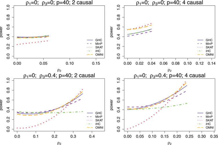
Power comparison of GHC, iHC, SKAT, MinP, and OMNI in hypothetical gene situations where there is no correlation within the causal variants (ρ₁ 0), for different correlations among the noncausal variants ρ₃, as a function of the correlation between the causal and noncausal variants ρ₂. Two sparsity levels were considered. Starting with ρ₂ = 0, power is estimated from 500 simulations for each possible ρ₂ > 0 that is a multiple of 0.01. There is a limit on how large ρ₂ can be relative to ρ₁ and ρ₃ so that the correlation matrix remains positive definite, and for this reason the range of ρ₂ values that power is estimated for varies with ρ₁ and ρ₃.

Figure 4.

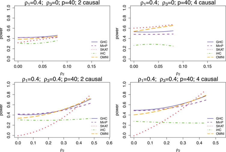
Power comparison of GHC, iHC, SKAT, MinP, and OMNI in hypothetical gene situations where the correlation within the causal variants is ρ₁ = 0.4 for different correlations among the noncausal variants ρ₃, as a function of the correlation between the causal and noncausal variants ρ₂. Two sparsity levels were considered. Starting with ρ₂ = 0, power is estimated from 500 simulations for each possible ρ₂ > 0 that is a multiple of 0.01. There is a limit on how large ρ₂ can be relative to ρ₁ and ρ₃ so that the correlation matrix remains positive definite, and for this reason the range of ρ₂ values that power is estimated for varies with ρ₁ and ρ₃.

Figures 3 and 4 GHC and MinP are more similar in performance to each other in most settings than they are to either SKAT or iHC. This is expected, because they are both tests designed for testing for a sparse alternative based on the extreme marginal test statistics while ignoring the less significant test statistics except for taking correlation of the region into account. On the other hand, iHC is based on the extreme transformed marginal test statistics, which tend to be quite different, and SKAT is a weighted sum of the squares of all the marginal test statistics. GHC improves in performance relative to MinP when ρ₁ increases, ρ₂ increases, or sparsity decreases. The iHC test has considerably lower power than GHC in most settings with correlation present. SKAT improves relative to MinP and GHC as sparsity decreases, but has very low power when ρ₂ is low while ρ₃ is large. The reason for this is because in this situation the noncausal variant block represents the direction of the first eigenvector of Σ, and the power of SKAT is very sensitive to this principal eigenvector direction, being nearly powerless when the signals are orthogonal to it. GHC and MinP do not rely heavily on the first few principal components of Σ and are robust due to their reliance on only the extreme test statistics. They receive only a slight penalty in power when taking the LD into account.

Overall, MinP is ideal when there are few causal variants and no LD in the region, and diminishes in power relative to other methods as sparsity decreases and the correlations between causal variants and noncausal variants (ρ₂) increase. SKAT does very well in low sparsity settings, but requires the causal variants to be in good correlation with the noncausal variants (ρ₂ ≫ 0). In fact, if the correlations between causal variants and noncausal variants (ρ₂) are sufficiently high, SKAT also works well even for high sparsity settings. However, where the correlation between causal variants and noncausal variants ρ₂ is weak and the correlation among the noncausal variants ρ₃ is not small, SKAT is subject to substantial power loss.

In contrast, GHC is very robust to all correlation structures and all sparsity levels. It outperforms iHC in the presence of correlation between SNPs in the region. GHC has a much higher power than SKAT especially in sparse settings when there are weak LDs between causal and noncausal variants (ρ₂ is small) and good LDs among noncausal variants (ρ₃ ≫ 0). GHC also outperforms MinP when sparsity decreases and the correlations between causal and noncausal variants (ρ₂) increase.

The omnibus test OMNI, as a pick-the-winner test, is also very robust. While it rarely is the strongest method, it always performs well in every setting. This is expected because in general an omnibus test should not be able to outperform the tests that contribute to it when the assumption of the contributing test is correct. While OMNI loses a little power compared to the most powerful candidate method, it is certainly the most robust choice when scanning the genome in the absence of prior knowledge of sparsity and LDs, as it can always borrow some of the strengths from GHC, MinP, and SKAT by adaptively accommodating different sparsity and LD structures of different genes across the genome.

7.3. Power Comparisons for a Large Number of Real Genes in a Chromosome

To compare power in a more realistic setting with more complex LD structures, power simulations are repeated on randomly selected genes from chromosome 5 using the 1000 cases and 1000 controls generated in the same fashion as (8). Genotype data are generated from common HapMap SNPs using the LD structure from the CEU population in the HapMap project using HapGen2 (Su, Marchini, and Donnelly 2011). Causal SNPs are selected at random from within each gene and the two sparsity settings considered are 2 causal variant and 4 causal variants, with each causal SNP given an effect size of β = 0.30 and β = 0.18, respectively. For each of the 839 genes inchromosome 5 containing more than 1 SNP, 100 simulations are used to estimate the power. Because the power will depend on the size of each gene, p, as well as the minor allele frequency of the causal SNPs, Figure 5 shows a smoothed power curve to represent the power averaged over all genes. In this case, ρ₂ is the median pairwise correlation between causal and noncausal variants. These results mirror the results from the block diagonal correlation structures in Figures 3 and 4 with the only difference being that power for all methods is lower for smaller ρ₂ in Figure 5 because in these realistic data lower correlation is often an artifact of low allele frequency which, in turn, leads to low power. This trend is not present in the block exchangeable setting considered in Figures 3 and 4, where allele frequency is fixed for all SNPs regardless of the correlation.

Figure 5.

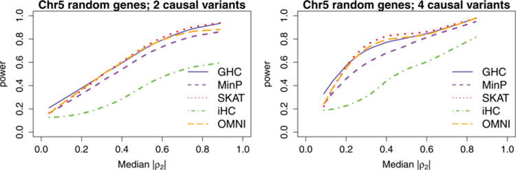
Power comparison of GHC, iHC, SKAT, and MinP for all the genes in Chromosome 5. For each of the 839 genes in chromosome 5, causal SNPs are selected at random and power is estimated at the α = 0.05 level based on 100 simulations. Additionally, the median correlation between causal SNPs and noncausal SNPs (ρ₂) is recorded. The smoothed curves to each of these power estimates is displayed.

Despite this, Figure 5 shows the results similar to those observed in Figures 3 and 4. As the LD between causal and non-causal variants increases, the powers of all the tests increase. GHC outperforms SKAT when signals are sparse and a gene has a weak LD, especially when the LDs between causal variants and noncausal variants (ρ₂) are weak. SKAT slightly outperforms GHC when signals become denser and a gene has stronger LD, especially when the LDs between causal variants and noncausal variants are strong. Both GHC and SKAT outperform MinP and iHC. GHC is robust to all correlation structures and sparsity levels. The omnibus test, as the pick-the-winner method, is more robust and performs well in all settings.

8. Application to the CGEM Breast Cancer Genetic Data

We compared the effectiveness of GHC to detect disease-associated genes with comparable methods using the breast cancer CGEM GWAS dataset described in the Introduction section. A total of 1145 postmenopausal women of Euro-pean ancestry with breast cancer and 1142 controls were included in the CGEM genome-wide association study (Hunter et al. 2007). These women were genotyped at 528,173 loci using an Illumina HumanHap500 array. The logistic regression model (1) was used while controlling for the covariates: age, post-menopausal hormone usage, and the top three principal components to correct for population stratification (Price et al. 2006).

Hunter et al. (2007) performed individual SNP analysis for this GWAS. Four SNPs in the FGFR2 region had marginal p-values less than 1.7 · 10⁻⁵ and none of them were close to genome-wide significance levels. The most significantly associated SNP in FGFR2 (rs1219648) was validated in further studies (Hunter et al. 2007; Stevens et al. 2006; Hayes et al. 2000; Eliassen et al. 2007). An SNP-set analysis can capture the amplified signal given off by multiple SNPs associated within the same gene.

To perform genome-wide gene-level analysis, for each gene, we group the SNPs within the gene as well as those in the 20 kb buffer region of the gene into an SNP-set. We applied five methods, GHC, iHC, SKAT, MinP, and OMNI, to analyze the GWAS data for gene-level analysis. The p-values for the five methods are displayed in Table 2 for genes with the most significant breast cancer associations. Only for these most significant genes was simulation of the null distribution used for calculating both OMNI and MinP p-values. To avoid the computational burden that simulation of the null distribution would require over a genome-wide analysis, OMNI was omitted and p-values for MinP were approximated using Moskvina and Schmidt (2008) in the Q–Q plot (Figure 6).

Table 2.

p-values of the most significant genes in analysis of the CGEM breast cancer GWAS using several gene-based tests: GHC, iHC, MinP, SKAT, and OMNI tests. The list is sorted in increasing order based on the smallest of the p-values of the tests that OMNI comprises of.

Gene	p	GHC	iHC	SKAT	MinP	OMNI
FGFR2	35	2.41 × 10−5	1.07 × 10−1	3.56 × 10−5	8.05 × 10−5	6.05 × 10−5
TBK1	11	3.47 × 10−4	3.86 × 10−3	5.63 × 10−5	8.39 × 10−4	1.02 × 10−4
PTCD3	12	5.77 × 10−5	1.11 × 10−3	1.15 × 10−4	2.18 × 10−4	1.04 × 10−4
POLR1A	16	6.90 × 10−5	1.35 × 10−2	3.97 × 10−4	3.10 × 10−4	3.09 × 10−4
CNGA3	26	2.37 × 10−4	1.14 × 10−3	1.09 × 10−4	1.12 × 10−3	2.68 × 10−4
XPOT	9	5.53 × 10−4	1.76 × 10−2	1.60 × 10−4	9.93 × 10−4	4.84 × 10−4
VWA3B	51	6.06 × 10−4	9.39 × 10−2	2.06 × 10−4	1.86 × 10−3	8.05 × 10−4
C11orf49	24	2.39 × 10−4	3.49 × 10−3	3.84 × 10−4	3.41 × 10−3	9.05 × 10−4
MMRN1	10	4.54 × 10−4	9.35 × 10−3	3.83 × 10−2	2.86 × 10−4	2.86 × 10−4
DGKQ	9	3.98 × 10−4	6.45 × 10−3	7.41 × 10−3	2.95 × 10−4	3.74 × 10−4
SCARB2	22	5.62 × 10−4	6.80 × 10−2	7.08 × 10−4	4.19 × 10−4	4.82 × 10−4
TMEM175	10	5.76 × 10−4	1.11 × 10−2	3.52 × 10−3	4.22 × 10−4	3.30 × 10−4
HCN1	36	8.65 × 10−4	8.14 × 10−3	1.85 × 10−2	4.24 × 10−4	4.25 × 10−4
AGMAT	5	4.83 × 10−4	3.26 × 10−3	4.62 × 10−4	5.62 × 10−4	5.62 × 10−4
NTSR1	32	4.74 × 10−4	7.17 × 10−3	7.13 × 10−3	2.43 × 10−3	9.10 × 10−4

Figure 6.

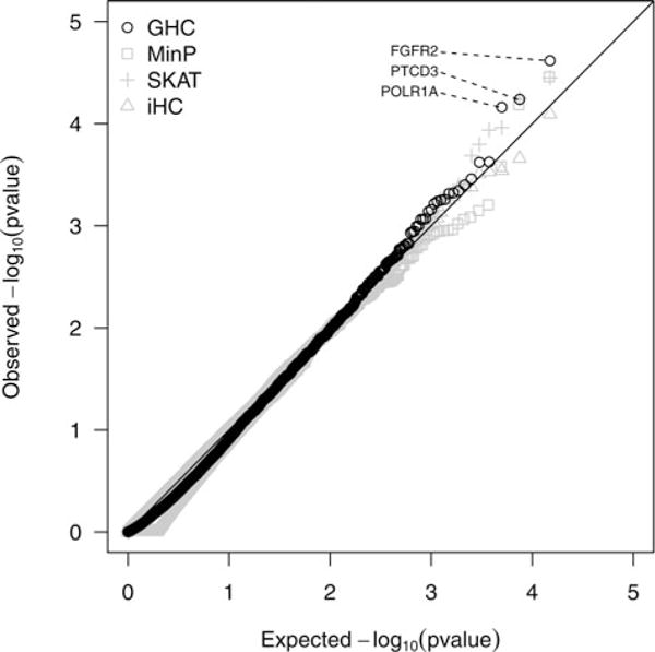
Q–Q plot of p-values for the SNP-set tests on the CGEM breast cancer GWAS data. SNP-sets were constructed at the gene-level, also including SNPs within 20 kb from the border of each gene. SNP-sets with 4 or fewer SNPs were not included in the analysis leading to total of 14,991 SNP-sets evaluated.

For the most significant gene, FGFR2, the GHC had the smallest p-value of 2.41 × 10⁻⁵. This p-value should not be directly compared with SNP-level p-values because there is less of a multiple testing problem (528,173 SNPs compared to 14,991 genes, which give a Bonferroni genome-wide SNP significance level 9.5 × 10⁻⁸ versus gene significance level 3.3 × 10⁻⁶). It should also be noted that the iHC p-value for FGFR2 is 0.107 which reflects the attenuated marginal test statistics seen in Figure 2. The second most significant gene, TBK1, is closely related to IKBKE, a known breast cancer oncogene (Boehm et al. 2007). For TBK1, SKAT detected the association with the smallest p-value of 5.63 × 10⁻⁵. The third most significant gene, PTCD3, has previously been identified in a gene network signifi-cantly associated with breast cancer (Jia et al. 2011). For PTCD3, the GHC had the most significant p-value of 5.77 × 10⁻⁵.

The FGFR2 gene is located on 10q26, and has a relatively weak LD structure overall, containing just one small LD block located between 123.35 Mb and 123.45 Mb. The four SNPs identified by Hunter et al. (2007) were not in this LD block, and although these SNPs were all in low LD with the rest of gene, the pairwise correlations among the four SNPs were all very strong (r² > 0.84). Due to the strong LD between these breast cancer-associated SNPs, it was concluded that there was a single breast cancer risk locus among them. In this case, iHC may not do well to detect the FGFR2 association because decorrelating the marginal test statistics would greatly deflate the signal given off by these four SNPs due to their strong LD. In contrast, this same correlation greatly benefits GHC as the noncausal SNPs are in high LD with the risk locus inherit and amplify the signal given off by the gene. The advantage gained by having four significant marginal test statistics in the numerator of (3) far outweighs the slight inflation of the variance term in the denominator. These differences are evidenced by the large disparity in the p-values of iHC and GHC for the FGFR2 gene. This is also similar to the situation with ρ₂ being small, and explains why GHC outperforms SKAT here. The signal is relatively dense with four strong marginal test statistics, and MinP is hurt by its failure to combine the strength of all four strong signals.

Overall, for the most significant genes (ordered by the minimum p-value of all four methods), MinP and iHC tended to yield less significant p-values than GHC and SKAT. SKAT and GHC both showed similar strength in detecting these top associations, but SKAT had some very insignificant p-values greater than 0.01 for a few of the top 15 genes (MMRN1 and HCN1) whereas GHC never had a p-value greater than 8.7 × 10⁻⁴. This difference demonstrates how GHC is more robust than SKAT to the LD in the top genes and is a safer bet in genome-wide association studies where there is a great variety of LD structures encountered. As expected, OMNI was the most robust method, whose p-values were closer to the most significant test (Table 2).

9. Discussion

In this article, we proposed the generalized higher criticism (GHC) test for testing for the effect of a genetic construct, such as a gene or a genetic pathway or network in genome-wide association studies. The GHC extends the higher criticism, an attractive detection method originally designed for testing for the global null hypothesis against a sparse alternative for independent data for high-dimensional problems, by accounting for correlation among SNPs in an SNP set. Unlike the original higher criticism, the GHC is flexible to SNP sets of arbitrary size and LD structure. We propose an analytic method to compute the p-values of GHC by accounting for correlation among the SNPs in an SNP set for finite samples that is computationally efficient and requires neither simulation nor asymptotics in p to obtain its p-values. This is advantageous when scanning a large number of genes in GWAS. An implementation of the method is freely available for use in the R package, GHC. We showed through simulation and analysis of the CGEM breast cancer GWAS data that the GHC is more robust to varied LD structures than competing methods, while ensuring appropriate Type I error control. In particular, we show that the GHC is more powerful than the iHC regardless of the LD structure.

As demonstrated by the simulation studies and the analysis of the breast cancer GWAS data, both GHC and SKAT complement each other well. GHC tends to outperform SKAT in the high sparsity settings especially when the correlations between causal variants and noncausal variants are weak and correlations among noncausal variants are moderate or strong. On the other hand, SKAT outperforms GHC when sparsity is low, especially when correlations between causal and noncausal variants are moderate or strong. This suggests that an omnibus test that combines the strengths of both GHC and SKAT could potentially be a powerful alternative in a variety of scenarios when scanning the genome. The robustness of such an omnibus test was demonstrated in our power simulations and analysis of the CGEM GWAS data. To make this test feasible for large-scale datasets like GWAS, it will be important to develop in the future a method of computing analytic p-values of the omnibus test or to develop computationally efficient software that can perform the required large-scale simulation of the null distribution.

Though our proposed analytic p-value calculations of GHC does not require asymptotics in p, asymptotics in the sample size N is assumed. The marginal test statistics are assumed to be normally distributed. However, this is a poor assumption if SNPs are rare, for example, in sequencing association studies (Lee et al. 2014) or if the sample size is small. For GWAS, this is not a problem due to their tendency to have large cohorts and only common SNPs genotyped.

We study in this article the detection boundary of GHC in the Gaussian linear regression case, as the detection boundary for the original higher criticism is well established in the previous literature (Donoho and Jin 2004; Ingster, Tsybakov, and Verzelen 2010; Arias-Castro, Candès, and Plan 2011). The recent work on the asymptotic properties of the original higher criticism for binary regression under sparse design matrices (Mukherjee, Pillai, and Lin 2015) shows that the detection boundary for binary regression is more complex. These results are not directly applicable for dense design matrices as observed in GWAS. It is of future research interest to study the detection boundaries of both the original higher criticism and GHC under dense design matrices for discrete outcomes in GLMs.

Advances in high-throughput sequencing technology are reshaping the field of genetics research, such as the 1000 Genomes Project and the NHGRI Genome Sequencing Program, as well as a rapidly increasing number of ongoing sequencing association studies. Indeed, candidate gene and whole genome sequencing studies have becoming rapidly available as the sequencing costs continue to drop. For sequencing association studies, as a vast majority of SNPs in the genome are rare, gene/region-based tests are often desirable (Lee et al. 2014). It is of future research interest to extend GHC region/gene-based tests to sequencing association studies to study for rare variant effects. To extend GHC to sequencing studies, the normality assumption of the marginal test statistics must be relaxed, and marginal test statistics that are robust to rare SNPs need to be developed by accounting for the nonnormality of the test statistics in finite samples when constructing the analog GHC region/gene-based tests for rare variant effects.

References

- Andrews DW, Pollard D. An Introduction to Functional Central Limit Theorems for Dependent Stochastic Processes. International Statistical Review/Revue Internationale de Statistique. 1994;62:119–132. [Google Scholar]
- Arias-Castro E, Candès E, Plan Y. Global Testing Under Sparse Alternatives: Anova, Multiple Comparisons and the Higher Criticism. The Annals of Statistics. 2011;39:2533–2556. [Google Scholar]
- Barnett IJ, Lin X. Analytical p-Value Calculation for the Higher Criticism Test in Finite-d Problems. Biometrika. 2014;101:964–970. doi: 10.1093/biomet/asu033. [DOI] [PMC free article] [PubMed] [Google Scholar]
- Boehm JS, Zhao JJ, Yao J, Kim SY, Firestein R, Dunn IF, Sjostrom SK, Garraway LA, Weremowicz S, Richardson AL, et al. Integrative Genomic Approaches Identify IKBKE as a Breast Cancer Oncogene. Cell. 2007;129:1065–1079. doi: 10.1016/j.cell.2007.03.052. [DOI] [PubMed] [Google Scholar]
- Chen H, Meigs JB, Dupuis J. Sequence Kernel Association Test for Quantitative Traits in Family Samples. Genetic Epidemiology. 2013;37:196–204. doi: 10.1002/gepi.21703. [DOI] [PMC free article] [PubMed] [Google Scholar]
- Conneely K, Boehnke M. So Many Correlated Tests, So Little Time! Rapid Adjustment of p-Values for Multiple Correlated Tests. The American Journal of Human Genetics. 2007;81:1158–1168. doi: 10.1086/522036. [DOI] [PMC free article] [PubMed] [Google Scholar]
- Crowder MJ. Beta-Binomial ANOVA for Proportions. Applied Statistics. 1978;27:34–37. [Google Scholar]
- Donoho D, Jin J. Higher Criticism for Detecting Sparse Heterogeneous Mixtures. The Annals of Statistics. 2004;32:962–994. [Google Scholar]
- Doukhan P. Mixing: Properties and Examples. Université de Paris-Sud, Département de Mathématique; 1991. [Google Scholar]
- Eliassen AH, Tworoger SS, Mantzoros CS, Pollak MN, Hankinson SE. Circulating Insulin and c-Peptide Levels and Risk of Breast Cancer Among Predominately Premenopausal Women. Cancer Epidemiology Biomarkers & Prevention. 2007;16:161–164. doi: 10.1158/1055-9965.EPI-06-0693. [DOI] [PubMed] [Google Scholar]
- Gaenssler P. Empirical Processes. Institute of Mathematical Statistics; 1983. [Google Scholar]
- Hall P, Jin J. Innovated Higher Criticism for Detecting Sparse Signals in Correlated Noise. The Annals of Statistics. 2010;38:1686–1732. [Google Scholar]
- Hayes RB, Reding D, Kopp W, Subar AF, Bhat N, Rothman N, Caporaso N, Ziegler RG, Johnson CC, Weissfeld JL, et al. Etiologic and Early Marker Studies in the Prostate, Lung, Colorectal and Ovarian (plco) Cancer Screening Trial. Controlled Clinical Trials. 2000;21:349S–355S. doi: 10.1016/s0197-2456(00)00101-x. [DOI] [PubMed] [Google Scholar]
- Hoeffding W, Robbins H. The Central Limit Theorem for Dependent Random Variables. Duke Mathematical Journal. 1948;15:773–780. [Google Scholar]
- Hunter D, Kraft P, Jacobs K, Cox D, Yeager M, Hankinson S, Wacholder S, Wang Z, Welch R, Hutchinson A, et al. A Genome-Wide Association Study Identifies Alleles in fgfr2 Associated With Risk of Sporadic Postmenopausal Breast Cancer. Nature Genetics. 2007;39:870–874. doi: 10.1038/ng2075. [DOI] [PMC free article] [PubMed] [Google Scholar]
- Ingster YI, Tsybakov AB, Verzelen N. Detection Boundary in Sparse Regression. Electronic Journal of Statistics. 2010;4:1476–1526. [Google Scholar]
- Ionita-Laza I, Lee S, Makarov V, Buxbaum JD, Lin X. Sequence Kernel Association Tests for the Combined Effect of Rare and Common Variants. The American Journal of Human Genetics. 2013;92:841–853. doi: 10.1016/j.ajhg.2013.04.015. [DOI] [PMC free article] [PubMed] [Google Scholar]
- Jaeschke D. The Asymptotic Distribution of the Supremum of the Standardized Empirical Distribution Function on Subintervals. The Annals of Statistics. 1979;7:108–115. [Google Scholar]
- Jia P, Zheng S, Long J, Zheng W, Zhao Z. dmgwas: Dense Module Searching for Genome-Wide Association Studies in Protein–Protein Interaction Networks. Bioinformatics. 2011;27:95–102. doi: 10.1093/bioinformatics/btq615. [DOI] [PMC free article] [PubMed] [Google Scholar]
- Leadbetter MR, Lindgren G, Rootzén H. Extremes and Related Properties of Random Sequences and Processes. Vol. 21. New York: Springer-Verlag; 1983. [Google Scholar]
- Lee S, Abecasis GR, Boehnke M, Lin X. Rare-Variant Association Analysis: Study Designs and Statistical Tests. The American Journal of Human Genetics. 2014;95:5–23. doi: 10.1016/j.ajhg.2014.06.009. [DOI] [PMC free article] [PubMed] [Google Scholar]
- Lee S, Wu MC, Lin X. Optimal Tests for Rare Variant Effects in Sequencing Association Studies. Biostatistics. 2012;13:762–775. doi: 10.1093/biostatistics/kxs014. [DOI] [PMC free article] [PubMed] [Google Scholar]
- Li B, Leal SM. Methods for Detecting Associations With Rare Variants for Common Diseases: Application to Analysis of Sequence Data. The American Journal of Human Genetics. 2008;83:311–321. doi: 10.1016/j.ajhg.2008.06.024. [DOI] [PMC free article] [PubMed] [Google Scholar]
- MacCullagh P, Nelder JA. Generalized Linear Models. Vol. 37. London: CRC Press; 1989. [Google Scholar]
- Manolio T, Collins F, Cox N, Goldstein D, Hindorff L, Hunter D, McCarthy M, Ramos E, Cardon L, Chakravarti A, et al. Finding the Missing Heritability of Complex Diseases. Nature. 2009;461:747–753. doi: 10.1038/nature08494. [DOI] [PMC free article] [PubMed] [Google Scholar]
- Moscovich-Eiger A, Nadler B, Spiegelman C. The Calibrated Kolmogorov-Smirnov Test. arXiv preprint arXiv:1311.3190 2013 [Google Scholar]
- Moskvina V, Schmidt K. On Multiple-Testing Correction in Genome-Wide Association Studies. Genetic Epidemiology. 2008;32:567–573. doi: 10.1002/gepi.20331. [DOI] [PubMed] [Google Scholar]
- Mukherjee R, Pillai NS, Lin X. Hypothesis Testing for High Dimensional Sparse Binary Regression. The Annals of Statistics. 2015;43:352–381. doi: 10.1214/14-AOS1279. [DOI] [PMC free article] [PubMed] [Google Scholar]
- Price AL, Patterson NJ, Plenge RM, Weinblatt ME, Shadick NA, Reich D. Principal Components Analysis Corrects for Stratification in Genome-Wide Association Studies. Nature Genetics. 2006;38:904–909. doi: 10.1038/ng1847. [DOI] [PubMed] [Google Scholar]
- Schwartzman A, Lin X. The Effect of Correlation in False Discovery Rate Estimation. Biometrika. 2011;98:199–214. doi: 10.1093/biomet/asq075. [DOI] [PMC free article] [PubMed] [Google Scholar]
- Stevens VL, Rodriguez C, Pavluck AL, Thun MJ, Calle EE. Association of Polymorphisms in the Paraoxonase 1 gene With Breast Cancer Incidence in the cps-ii Nutrition Cohort. Cancer Epidemiology Biomarkers & Prevention. 2006;15:1226–1228. doi: 10.1158/1055-9965.EPI-05-0930. [DOI] [PubMed] [Google Scholar]
- Su Z, Marchini J, Donnelly P. Hapgen2: Simulation of Multiple Disease Snps. Bioinformatics. 2011;27:2304–2305. doi: 10.1093/bioinformatics/btr341. [DOI] [PMC free article] [PubMed] [Google Scholar]
- Visscher PM, Brown MA, McCarthy MI, Yang J. Five Years of Gwas Discovery. The American Journal of Human Genetics. 2012;90:7–24. doi: 10.1016/j.ajhg.2011.11.029. [DOI] [PMC free article] [PubMed] [Google Scholar]
- Wu M, Lee S, Cai T, Li Y, Boehnke M, Lin X. Rare-Variant Association Testing for Sequencing Data With the Sequence Kernel Association Test. The American Journal of Human Genetics. 2011;89:82–93. doi: 10.1016/j.ajhg.2011.05.029. [DOI] [PMC free article] [PubMed] [Google Scholar]
- Wu MC, Kraft P, Epstein MP, Taylor DM, Chanock SJ, Hunter DJ, Lin X. Powerful SNP-set Analysis for Case-Control Genome-Wide Association Studies. The American Journal of Human Genetics. 2010;86:929–942. doi: 10.1016/j.ajhg.2010.05.002. [DOI] [PMC free article] [PubMed] [Google Scholar]
- Wu Z, Sun Y, He S, Cho J, Zhao H, Jin J, et al. Detection Boundary and Higher Criticism Approach for Rare and Weak Genetic Effects. The Annals of Applied Statistics. 2014;8:824–851. [Google Scholar]
- Zhang Y, Liu J. Fast and Accurate Approximation to Significance Tests in Genome-Wide Association Studies. Journal of the American Statistical Association. 2011;106:846–857. doi: 10.1198/jasa.2011.ap10657. [DOI] [PMC free article] [PubMed] [Google Scholar]
- Zhong PS, Chen SX, Xu M, et al. Tests Alternative to Higher Criticism for High-Dimensional Means Under Sparsity and Column-Wise Dependence. The Annals of Statistics. 2013;41:2820–2851. [Google Scholar]
Associated Data
This section collects any data citations, data availability statements, or supplementary materials included in this article.