Urbanization-induced population migration has reduced ambient PM_2.5 concentrations in China

Population migration has upgraded the direct energy consumption with remarkable benefits on air quality and health in China.

Abstract

Direct residential and transportation energy consumption (RTC) contributes significantly to ambient fine particulate matter with a diameter smaller than 2.5 μm (PM_2.5) in China. During massive rural-urban migration, population and pollutant emissions from RTC have evolved in terms of magnitude and geographic distribution, which was thought to worsen PM_2.5 levels in cities but has not been quantitatively addressed. We quantify the temporal trends and spatial patterns of migration to cities and evaluate their associated pollutant emissions from RTC and subsequent health impact from 1980 to 2030. We show that, despite increased urban RTC emissions due to migration, the net effect of migration in China has been a reduction of PM_2.5 exposure, primarily because of an unequal distribution of RTC energy mixes between urban and rural areas. After migration, people have switched to cleaner fuel types, which considerably lessened regional emissions. Consequently, the national average PM_2.5 exposure concentration in 2010 was reduced by 3.9 μg/m³ (90% confidence interval, 3.0 to 5.4 μg/m³) due to migration, corresponding to an annual reduction of 36,000 (19,000 to 47,000) premature deaths. This reduction was the result of an increase in deaths by 142,000 (78,000 to 181,000) due to migrants swarming into cities and decreases in deaths by 148,000 (76,000 to 194,000) and 29,000 (15,000 to 39,000) due to transitions to a cleaner energy mix and lower urban population densities, respectively. Locally, however, megacities such as Beijing and Shanghai experienced increases in PM_2.5 exposure associated with migration because these cities received massive immigration, which has driven a large increase in local emissions.

INTRODUCTION

Air pollution in China causes 1 million premature deaths each year and ranks first among many environmental concerns in terms of health (1–3). Among various sources that are attributable to air pollution, direct energy consumption in residential and transportation sectors (referred to as “RTC” in this study) contributes significantly to the emissions of air pollutants, such as carbon monoxide (CO), nitrogen oxide (NO_x), sulfur dioxide (SO₂), black carbon (BC), organic carbon (OC), and benzo[a]pyrene (4–8).

Unlike emissions from other sources, emissions from RTC are determined by the time, location, and intensity of residents’ daily activities and, therefore, are spatially correlated with population distribution. Given the same level of emissions, RTC emissions are associated with higher levels of population exposure compared to other sources, because of their proximity to people (9, 10). Hundreds of millions of people have moved into cities over the past three decades of rapid urbanization in China (11). This massive rural-urban migration has significantly altered the spatial distribution of RTC emissions and population exposure for multiple reasons. First, rural-urban migration is associated with a spatial relocation of RTC pollutant emissions from rural areas to cities. The tendency of both emissions and the number of population exposed to these emissions to increase in cities has important impacts on public health. Second, the amount of per-capita RTC emissions tends to be reduced by migration because the migrating population transitions to a cleaner energy mix. For example, most migrants abandon the use of biomass fuel after settling down in cities and, instead, use energy sources or fuels that emit fewer air pollutants (11, 12). These two processes are competitive in terms of population health.

Specific influences of rural-urban migration on pollutant emissions and health consequences have not been quantified to date in China, mainly due to the lack of long-term spatially explicit data. Here, we analyze the influence of the massive rural-urban migration on pollutant emissions from RTC sources and population exposure to these emissions from 1980 to 2012 in the country. We chose the year 1980 as the beginning of our study period because it corresponds to the date when urbanization started to accelerate following the initiation of the Chinese economic reform and opening policy (11). We then evaluate the resulting health impacts during the same period and forecast the likely changes in these health impacts to the year 2030. We only focus on RTC emissions. Influences of migration on other pollution sources and the subsequent health impacts are beyond our scope.

RESULTS

Integrated model framework

Rural-urban population migration is associated with urban land expansion, increased urban RTC emissions, decreased rural RTC emissions, and increased number of people being exposed to polluted urban air. The impact of migration is thus a combined consequence of different changing factors (Fig. 1). On the basis of accountability analyses (13), we carry out model simulations for two scenarios to evaluate the impact of migration. One is the real-world scenario that considers all historical and future-projected changes in population distribution and RTC energy mix during the study period from 1980 to 2030. The other is a counterfactual scenario that assumes that no migration happened since 1980. In this scenario, the per-capita urban and rural RTC energy mixes for a given year are consistent with those in the real-world scenario, but the proportions of urban population are increasingly lower over time. We evaluate the net impacts of migration based on cross-sectional comparisons of the total RTC energy mixes, pollutant emissions, particulate matter with a diameter of 2.5 μm or less (PM_2.5) concentrations (primary and secondary), and premature deaths between the two scenarios. We find that the disparity between urban and rural RTC energy mix is critical because it determines how much rural emissions will be decreased by migration compared to the increase in urban emissions (Fig. 1; discussed in detail in subsequent sections). To quantify the assessment, we characterize the urban and rural RTC per capita and total energy mixes, the geographical distributions of rural-urban migration, emissions of primary PM pollutants and secondary PM precursors, and population exposure to ambient PM_2.5. We investigate their changes over time using remote sensing data, air quality monitoring data, official statistical data, and questionnaire survey data. We use a series of energy statistical models, an air quality model, and a Gaussian downscaling method to integrate these data for evaluation. We conduct comprehensive sensitivity and uncertainty analyses to address the uncertainty in the emission estimation, air quality modeling, and health risk assessment. A detailed description of this integrated model framework is provided in Materials and Methods.

Fig. 1. Illustration of the changes in urban and rural RTC emissions and PM_2.5 concentrations due to population migration.

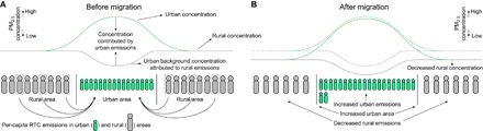
Distributions of RTC emissions and PM_2.5 concentrations before (A) and after (B) migration. Compared with rural areas, urban areas are associated with lower per-capita RTC emissions due to cleaner RTC energy mix used by the urban population. A consequence of the population migration is the decrease in rural population density, which leads to decreases in RTC emissions and PM_2.5 concentration in rural areas. In contrast, migration-induced change in urban concentration is a competition between increased urban emissions and declined background concentrations contributed by decreased rural emissions. In addition, migration to cities causes more people to be exposed to polluted urban air. The overall change in population exposure concentration and premature deaths across China due to migration is the consequence of the concurrent changes in both concentrations and population distributions.

Changes in population

On the basis of the unique registration system (hukou) of citizens in China, urban population can be classified into three categories: (i) OUs, old urban residents registered with urban hukou before 1980; (ii) NUs, new urban residents who are rural-urban migrants and got an urban hukou after 1980; and (iii) MUs, unregistered rural-urban migrants who live in cities without an urban hukou. When rural residents (RRs) who live in rural areas migrate to cities, they become either NUs or MUs, depending on whether they can get an urban hukou. With a hukou, NUs have a lifestyle similar to that of OUs, and their energy mix changes accordingly. By contrast, MUs who do not have an urban hukou have limited access to urban energy infrastructure, social welfare, and other city services. Our surveys show that the energy mix of MUs is very different from that of OUs and NUs, and because they lose access to biomass fuels when they move to the city, MUs use an energy mix different from that of the RRs as well (12).

From 1980 to 2013, the urbanization rate in China, equal to (OU + NU + MU)/(OU + NU + MU + RR), rapidly increased from 19.4 to 53.7% (11). Fractions of OUs, NUs, MUs, and RRs changed markedly (Fig. 2A), coincident with an increase of 380 million in the total population. The total number of rural-urban migrants (NU + MU) increased from virtually zero in 1980 to 485 million in 2013, split between 341 million NUs and 144 million MUs. Consequently, the population distribution shifted from low-density rural areas to high-density urban areas (Fig. 2B). It is predicted that another 254 million RRs, including 38 million MUs, will settle in cities, pushing the urbanization rate up to 70% by 2030 (14, 15). Meanwhile, from 1980 to 2013, the total number of OUs remained relatively constant because of their very low birth rate, which was constrained by the one-child policy (16). The population in rural areas, where out-migration surpassed increasing net birth rates, decreased since the early 1990s.

Fig. 2. The rapidly changing population in China from 1980 to 2030.

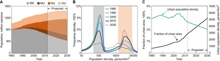
(A) Temporal trends of the population of four major categories. (B) Temporal trends of the urban population density and the fraction of urban areas to total area. (C) Population frequency distributions at different levels of population densities in 1980, 1990, 2000, 2010, and 2030. The gray and orange regions illustrate the population density ranges containing most of the rural and urban population, respectively.

We recognize urbanization as a phenomenon that manifests in terms of both increasing urban population and expanding urban land cover across the landscape (see Materials and Methods and figs. S1 and S2). We find that urban areas increased from less than 0.4% of the total country area in 1980 to 1.7% in 2013 (Supplementary Materials). The urban area fraction is projected to reach almost 3% in 2030 (Fig. 2C). The increase of urban area accelerated after around 2007, when the mean annual income of urban residents reached US$2000 per capita (in constant 2005 US$) and real estate started to boom (11). Because of higher income and the stronger demand for larger floor area per capita and more public space (11), urban area increased at a faster pace than urban population, leading to an overall decrease in urban population density (Fig. 2C).

Changes in RTC energy mix

Because of differences in lifestyle, income, and access to various energy resources, RTC energy mixes differ between urban and rural dwellers. We combine OUs and NUs as a single urban resident (UR) group because NUs attain a social status similar to that of OUs as a result of their hukou registration and the two groups’ energy mixes are expected to be comparable. By analyzing energy mixes of the three groups (URs, MUs, and RRs), we find that, in China, RRs still rely on biomass fuels (72% in 2010; see Materials and Methods), including crop residue and firewood, and their per-capita energy consumption is high (Fig. 3A) because of the low efficiency of biomass fuel combustion. URs use a large quantity of fuel oil for transportation, and their per-capita energy consumption is the highest among the three groups. MUs have the lowest per-capita consumption among the three groups. The per-capita energy consumption of URs and MUs in the north of China is higher than that in the south, mainly due to their greater use of coal and heat. Nevertheless, our questionnaire survey showed that MU households in northern China are still underheated. Sixteen percent of the MUs in Beijing do not heat their home in winter at all, relying only on electric blankets (12). The MU energy mix is very different from the UR energy mix in northern China, where more coal and less gas and heat are used by MUs (Fig. 3A) as a result of limited access to natural gas distribution networks and centralized heating systems (12). In general, differences in socioeconomic status yield large disparities in RTC energy mixes between URs and RRs; MUs represent a transition stage from the solid fuel–dominant rural energy mix to the clean fuel–dominant urban energy mix.

Fig. 3. Disparities in RTC energy consumption among RRs, MUs, and URs.

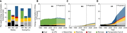
(A) Per-capita energy mix of RRs, MUs, and URs in Beijing (a representative for the north of China) and Guangzhou (a representative for the south of China). Beijing and Guangzhou are the two cities where our questionnaire surveys were conducted. The per-capita energy consumption of RRs is calculated as the weighted average of per-capita rural energy consumption of all home provinces of the rural-urban migrants in that city. (B) Temporal trend of total RTC energy consumption by RRs in China. (C) Temporal trend of total RTC energy consumption by MUs in China. (D) Temporal trend of total RTC energy consumption by URs in China.

Driven by important economic changes, the RTC energy mix has changed rapidly since 1980. We find differential changing patterns between URs and RRs, as is shown in fig. S3 where we plot the per-capita RTC consumption against the per-capita gross domestic product (GDP_cap) using provincial-level statistical data from 1980 to 2012. Although the per-capita consumption of clean energy (all fuel types excluding solid fuels) among both URs and RRs, except heat, which is not available in rural areas, has increased as GDP_cap increases, the consumption of RRs started at a much lower level and would only catch up with that of URs when GDP_cap reached a value of around US$10,000 (in constant 2005 US$) (fig. S3). In rural China, both liquefied petroleum gas (LPG) and electricity have been progressively adopted for cooking because of their low prices (17) and high accessibility due to the adequate power grid and road networks. In 2009, 99.4% of villages were connected with paved roads (18), and in 2013, 99.6% of rural residences were connected to electric grids (19). Meanwhile, the per-capita solid fuel consumption decreased rapidly in urban areas but remains almost constant in rural areas between 1980 and 2012 (fig. S3). Encouraging the transition from coal and biomass to other energy sources is the biggest challenge in promoting clean energy in rural China. Because of data limitations, there is more uncertainty in the trends of the energy mix of MUs than the other two groups of people. Here, we use the data from Ru et al. (12), which indicate that the MU energy mix changed much more slowly during the last three decades than the UR, likely due to the former’s unchanged social status and living conditions.

The total RTC energy mixes of URs and RRs show very distinct patterns over time (Fig. 3, B to D). For the URs, the consumption of all fuel types except coal has increased markedly after the mid-2000s because of the increase of per-capita energy use (accounting for 65% of the overall increase) and the increase of UR population (34%). For the RRs, there is no significant change in the total amount of energy consumption because the decrease in biomass consumption is nearly compensated by the increase in the consumption of electricity and LPG. Compared to the gradual transition of the rural energy mix, the energy mix in urban areas has been shifting faster toward a higher share of clean fuels since the early 1990s. Because of the fast energy transition in the urban area and the increasing proportion of urban population due to population migration, RTC energy consumption in China has increased at a fast pace with the energy structure shifting from being solid fuel–dominated (95% in 1980) toward becoming cleaner energy–dominated (62% in 2013). Population migration has facilitated this process by providing more people with easier access to clean fuels. According to our estimate, without the three decades–long migration, solid fuel would still be the dominant fuel type, accounting for 60% of the total RTC energy consumption today (see Materials and Methods). Our findings suggest that population migration and associated policies will continue to drive the energy demand and, to a large extent, the energy mix in the decades to come.

Influences of population migration on pollutant emissions and PM_2.5 concentrations

On the basis of the per-capita energy mix (Fig. 3), we estimate the per-capita emissions of primary PM pollutants and secondary PM precursors among the URs, MUs, and RRs (see Materials and Methods for the emission estimation and spatial allocation, and note that emissions from electricity consumption are spatially allocated to the locations of individual power plants). Disparities in the RTC energy mix among the three groups lead to differential pollutant emission profiles (Fig. 4). For SO₂, which has a higher emission factor (EF; defined as the emission per unit energy consumption) for electricity, which is generated predominantly by coal-fired power plants in China, than for other fuel types, the per-capita emissions of URs and MUs are higher than those of RRs because of the higher share of electricity consumption of URs and MUs. For NO_x, which has high EFs for both electricity consumption and transportation, the per-capita emissions of URs are the highest. For most other pollutants, including all primary PM pollutants and other secondary PM precursors, solid fuels have a much higher EF than other fuel types. Therefore, RRs have the highest per-capita emissions because of their higher share of solid fuels. Therefore, except for SO₂ and NO_x, the direct result of the migration from rural to urban areas is an overall reduction in emissions of most PM-related pollutants.

Fig. 4. Per-capita RTC emissions of primary PM pollutants and secondary PM precursors in China by fuel.

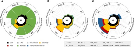
Per-capita RTC emissions of RRs (A), MUs (B), and URs (C). The axis ranges of different pollutants are different, as shown in the legend. The per-capita emissions shown in the graphs are national averages in 2010. See figs. S4 and S5 for the per-capita emissions in 1990 and 2030. NMVOC, non-methane volatile organic compounds; TSP, total suspended particulate matter.

The massive rural-urban migration and the changes in the energy mix of migrants as they settle in urban areas have caused remarkable changes in the pollutant emissions and PM_2.5 concentrations across China. Given the higher health concerns from PM_2.5, we show here the changes in the PM_2.5 (primary) emissions and the PM_2.5 (primary + secondary) concentrations in 2010 caused by population migration between 1980 and 2010 (see Materials and Methods). In rural areas, decreases in the population due to out-migration to urban areas have caused an annual reduction of 2.8 Tg in PM_2.5 emissions from RTC sources. In the meantime, there has been a corresponding increase in PM_2.5 emissions in the urban areas but of a considerably smaller magnitude owing to the newly arriving migrants upgrading their energy mix. We estimate that the increase in urban PM_2.5 emissions was 0.5 Tg, which equated to only 18% of the reduction in rural emissions. Hence, there was a net reduction of 2.3 Tg in PM_2.5 emissions in 2010, owing to the rural-urban migration. Transitions of RRs to NUs and MUs contributed 70 and 30%, respectively, to the net emission reduction.

Spatially, all cities showed an increase in PM_2.5 emissions due to migration, with a higher level of the emission increase occurring in megacities across China and most cities in the North China plain (Fig. 5A). On the other hand, PM_2.5 emission per unit urban area decreased in most cities because the extent of the cities expanded faster than their urban PM_2.5 emissions did. The few exceptions were mostly located in the southwest, where the increase in urban area was slower than the increase in migration-induced urban emissions and the emission intensities eventually increased. The relative change in the rural area is much smaller than that in the urban area, considering that, in China, a 100% increase in the urban area corresponds to a 0.6% decrease in the rural area. Thus, the loss of rural population directly led to the decrease in rural population density. Both rural PM_2.5 emission and PM_2.5 emission density decreased accordingly. This is particularly true for the regions that contributed dominantly to the out-migration of migrants such as Sichuan and Anhui provinces. Unlike the primary PM_2.5 emissions, the emissions of the secondary PM precursors, including SO₂ and NO_x, slightly increased in response to migration due to their higher per-capita emissions among the urban population, as mentioned above.

Fig. 5. Migration-induced spatial changes in PM_2.5 emissions and concentrations in China.

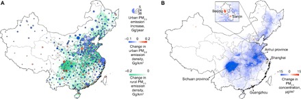
Spatial changes in (A) annual primary PM_2.5 emissions and (B) annual average PM_2.5 concentrations (primary + secondary) in 2010 in mainland China caused by the population migration in the last 30 years. (A) The bubbles represent the changes in emissions within the urban areas of individual cities. The areas of the bubbles are proportional to emission increase. The color of the bubbles shows the change in urban emission density. Emission change in rural area is shown in the background. Because of population migration since 1980, emissions from RTC were spatially relocated. Rural emissions decreased pervasively while urban emissions increased. The national total emissions were also changed by migration because migrants got easier access to clean fuels and spontaneously shifted their energy mix after migrating into urban areas. (B) Migration-induced increase in urban emissions cannot compensate the extensive decrease in rural areas, leading to a reduction of PM_2.5 concentrations across the east part of the country. There are some exceptions such as those four megacities. Serving as the destinations of massive migration, these cities showed an increase in PM_2.5 concentrations due to increased local emissions by migration.

Considering all PM-related pollutants, we evaluate the migration-induced change in PM_2.5 concentration (primary + secondary) in 2010 across China at a 5-km × 5-km spatial resolution, which is fine enough to capture the urban and rural changing patterns separately (see Materials and Methods) (Fig. 5B). In rural areas, population migration has caused a pervasive reduction in PM_2.5 concentrations over the central and eastern part of China. In most urban areas, decreases in background concentrations surpassed the influence of increased local emissions, leading to an overall improvement in urban PM_2.5 concentrations as well. In contrast, megacities, including Beijing, Tianjin, Shanghai, and Guangzhou, experienced increases in PM_2.5 concentrations because these cities are the major destination of migrants; that is, even with the reduction in background concentrations, the numbers of migrants were so large that, overall, the PM_2.5 concentrations were significantly elevated owing to the migration-induced increase in local emissions.

Influences on exposure and health

By analyzing the difference in simulated exposure to PM_2.5 before and after migration, we find that the overall population exposure to PM_2.5 has decreased because of the migration-induced change in RTC emissions. For example, the national average exposure concentration was 58.6 μg/m³ in 2010. It would have been 62.5 μg/m³, had the rural-urban migration not happened and the migrants still relied on rural RTC mix in their rural households. A direct consequence of this difference has been an annual reduction of 36,000 (90% confidence interval, 19,000 to 47,000) premature deaths in China in 2010 and a cumulative reduction of 450,000 (195,000 to 490,000) premature deaths from 1980 to 2010 (see Materials and Methods), indicating a health benefit from the three decades of migration. Migration benefited both urban and rural populations; the reduction in the exposure concentrations was 7.2 μg/m³ (5.0 to 11.4 μg/m³) and 7.4 μg/m³ (5.7 to 10.0 μg/m³) in urban and rural areas, respectively. The reason why the reduction in urban and rural areas is comparable is that, as urban areas expanded, surrounding areas with lower levels of concentrations were included in the assessment of urban exposure and contributed to an additional reduction in the calculated exposure level. Our findings indicate that the migration-induced reductions in PM_2.5 exposure concentrations over China essentially started from the early 1990s; these reductions are expected to reach up to 8.8 μg/m³ by 2030, doubling the current benefits on air quality and health (fig. S6).

Although the total PM_2.5 (primary + secondary) concentration decreased with migration, secondary PM_2.5 did not decrease simultaneously. Instead, we find steady increases in secondary PM_2.5 caused by migration in the metropolitan areas of the Pearl River Delta (3.8 μg/m³), Beijing-Tianjin-Tangshan (1.3 μg/m³), and the Yangtze River Delta (1.2 μg/m³) as a result of increased emissions of secondary PM precursors such as NO_x and SO₂ from power generation and motor vehicles. This is consistent with the recent observations showing that secondary aerosols are playing an increasingly prominent role in urban air degradation in China (20, 21).

Simulated changes in PM_2.5 (primary + secondary) concentrations in the urban areas across China varied from −30 to 5 μg/m³ (Fig. 6). We find that the exposure reduction is related to both socioeconomic and climatic factors. The migration-induced decline in the PM_2.5 exposure is more pronounced in cities with a moderate level of GDP_cap (Fig. 6A). Both the least-developed and the most-developed cities benefit much less from the migration in terms of reduced PM_2.5 exposure. The least-developed cities attract few migrants, whereas the most-developed ones must cope with massive migration such that population densities remain high, precluding any reduction in exposure. Another important factor affecting the change in exposure during migration is the number of heating degree day (HDD) (Fig. 6B) (22). Higher HDD is associated with a smaller reduction in PM_2.5 concentration because, in cities in colder climates, new migrants use relatively more energy for heating compared to those in cities in warmer climates. Coal, a type of solid fuel that emits more pollutants, is usually used by migrants as an alternative fuel when other heating options are not available.

Fig. 6. Changes of PM_2.5 exposure concentrations in urban areas of individual cities as a result of population migration in 2010.

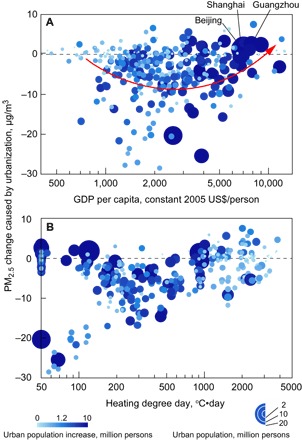
Each bubble represents an individual city. The areas of the bubbles are proportional to urban population in the city. The shades of the bubbles represent the increase in urban population since 1980. (A) Relationship between the migration-induced change in PM_2.5 exposure concentrations with GDP_cap. (B) Relationship between the migration-induced change in PM_2.5 exposure concentrations with HDD.

Attribution to individual migration-related and non–migration-related factors

Our evaluation showing the reduction in ambient PM_2.5 in 2010 is based on the simulation of a counterfactual scenario by excluding the migration and the change in RTC emissions caused by migration alone. However, other factors that are not related to migration, such as population growth and the increase in per-capita energy consumption, can also affect energy-related emissions and PM_2.5 concentrations. When considering the overall change of emissions from RTC, we find an increasing trend of ambient PM_2.5 concentration during the last three decades (fig. S6). To compare the migration-induced effects with other factors, we involve all of the changes in RTC sources, derive four factors that are unrelated to migration and five that are related, and evaluate their incremental effects on emissions, exposure concentrations, and mortality during the study period. The four factors unrelated to migration are population growth (N1), increase in per-capita RTC energy use (N2), change in RTC energy mix due to improvement in living conditions (N3), and decrease in EFs due to technology development (N4). The five migration-related factors are relocation and energy mix shift of the NU group (U1 and U2) and the MU group (U3 and U4) and urban area expansion (U5) (see Materials and Methods). We find that the exposure to PM_2.5 is enhanced by factors N1, N2, U1, and U3, whereas they are reduced by factors N3, N4, U2, U4, and U5.

The influences of these nine factors on PM_2.5 emissions, PM_2.5 exposure concentrations, and annual deaths from exposure to ambient PM_2.5 in 2010 are presented in Fig. 7. Of the four non–migration-related factors, the increase of per-capita energy use leads to a marked increase in the exposure in both urban and rural areas, given that per-capita RTC energy consumption has increased by 49.6 and 64.2% in urban and rural China, respectively (11). On the contrary, exposure concentrations are brought down by EF reductions due to advances in technology. For example, the EFs of PM_2.5 for cars have been reduced by 80% during the study period, along with continuously tightened regulations (23). In addition, stove improvement campaign has significantly increased the efficiency of millions of stoves in rural China (24). The overall consequence of all non–migration-related factors was an exposure increase of 7.8 μg/m³ (6.0 to 10.6 μg/m³) between 1980 and 2010.

Fig. 7. Influences of individual non–migration-related and migration-related factors on PM_2.5 emissions, PM_2.5 exposure concentrations, and annual deaths from exposure to ambient PM_2.5 in China in 2010.

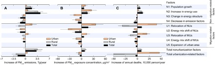
The results are presented as changes in PM_2.5 emissions (A), PM_2.5 exposure concentrations (B), and annual deaths from exposure to ambient PM_2.5 (C) caused by the change of individual non–migration-related and migration-related factors between 1980 and 2010. Influences on urban, rural, and total areas are illustrated using bars with different colors. In urban areas, total migration-related factors led to a decrease in PM_2.5 exposure concentration but an increase in annual deaths because the urban population base was increased as a result of migration.

Among the migration-related factors, spatial relocation and shift in energy mix of NUs contribute the most to the increase and decrease in the exposure, respectively, primarily in urban areas. The influence of the energy mix change for MU is important, although to a lesser extent. In addition, the decrease in the urban population density caused by urban expansion is also responsible for the reduction in the urban PM_2.5 exposure concentration. In terms of population health, the spatial relocation of migrants (U1 + U3) was responsible for an increase of 142,000 (78,000 to 181,000) deaths in 2010, whereas the energy mix change (U2 + U4) and urban expansion (U5) led to decreases of 148,000 (76,000 to 194,000) and 29,000 (15,000 to 39,000) deaths, respectively. The overall consequence of all migration-related factors was a reduction in exposure of 3.9 μg/m³ (3.0 to 5.4 μg/m³) and a decrease in premature deaths by 36,000 (19,000 to 47,000) in China in 2010.

The urban and rural populations have benefited differently from the rural-urban migration. For example, relocation of MUs (U1) led to a large increase in PM_2.5 exposure concentration (35.6 μg/m³) in the urban areas but a small decrease (−0.6 μg/m³) in the rural areas, whereas the shift in the energy mix of MUs (U2) caused a reduction of 33.4 and 4.8 μg/m³ in exposure concentrations in the urban and rural areas, respectively. In general, effects of various migration-related factors are more pronounced in the urban areas owing to relatively high population and emission densities compared to those in the rural areas. Without migration, the overall change in emissions from RTC would have led to an increase of 7.8 μg/m³ in population exposure to ambient PM_2.5 between 1980 and 2010 in China. Given that the consequence of all migration-related factors is a decrease of 3.9 μg/m³ in exposure to ambient PM_2.5, migration has compensated for 50% of the increase in PM_2.5 exposure concentration on a national scale.

DISCUSSION

Focusing on RTC sources, our study reveals that rural-urban migration is a unique process in China that has reduced the national overall PM_2.5 concentration and exposure of population to PM_2.5 during the last 30 years despite the increase in both urban emissions and population being exposed to urban air. The fundamental causation comes from the uneven distributions of clean fuel accessibility for RTC between urban and rural areas, which is typical of China and other developing countries. The observed migration has bridged the transition from solid fuel–dominant rural energy mix to clean fuel–dominant urban energy mix, leading to a reduction in pollutant emissions and improvement of regional air quality.

Still, issues regarding migrants remain. In particular, MUs lack access to clean fuel sources because of the hukou registration system. They do not only end up contributing significantly to the emissions of air pollutants, which the entire urban population is exposed to, but also live in the so-called urban villages where air quality is often worse than other parts of the cities (25). This is particularly true in the northern cities where many of the MUs still rely on coal stoves for heating in winter (12). With the current hukou registration system in operation, it is almost impossible to provide them with better alternatives. A reform of this system has been discussed in a number of cities without much progress toward a solution (26). New strategies against this deep-rooted hukou system should be developed to diminish the socioeconomic status and welfare disparities between registered and unregistered urban residents. In addition, construction of urban energy infrastructure that can balance the RTC energy mix between registered and unregistered residents would remarkably improve urban air quality.

In China, as elsewhere in the world, cities experiencing rapid growth and economic development often face severe air pollution issues (27). Our study reveals that rural-urban migration is an important factor leading to air pollution in large cities that attract many more migrants than smaller cities do. Migration factors into the degradation of air quality in those cities because of significant increases in local pollutant emissions. Urban land expansion can help reduce population densities and exposure concentrations, only if it can be managed well, given that land is precious in China for sustainable agricultural and ecological conservation (28, 29). A recent study found that urban density can influence energy use as much as efficiency improvements such as transitioning to cleaner energy mixes (30). From orderly urban expansion to improvements in transportation system to upgrading the RTC energy mix and industrial-residential codevelopment (31, 32), there are options available for urban planning and governance to comprehensively address air quality issues in the context of rural-urban migration. Effectively harnessing the air quality dividends from rural-urban migration will benefit both rural and urban residents and will contribute to improving the quality of life in Chinese cities.

MATERIALS AND METHODS

Quantification of China’s urban expansion from 1980 to 2030

Although numerous studies have focused on urbanization in China, a comprehensive geospatial data set recording urban expansion since the beginning of China’s reform and opening up is still lacking. Spatially, to extract urban areas (or built-up areas), we used two types of data sources, including the remote sensing data and the nighttime light (NL) data. The former is represented by the Landsat Multispectral Scanner System, Thematic Mapper, and Enhanced Thematic Mapper, and the latter is represented by the Defense Meteorological Satellite Program’s Operational Linescan System (DMSP OLS) (33, 34). However, the Landsat data are limited by the spatial coverage and labor-consuming extraction procedures, whereas the NL data are limited by the spatial uncertainty and temporal coverage (recorded only after 1992). Here, we combined these two sets of data to extract urban expansion across China from 1980 to 2012. The future projection used here was derived according to future urban expansion forecasts in a previous study (29).

To derive urban area from NL digital values, threshold values need to be determined. However, given the spatial difference in socioeconomic characteristics in China, a single threshold cannot be applied to all regions and years. For the year 2010, we calculated the fractions of urban built-up areas of individual counties based on the Landsat-based product of Global Land Cover maps with 30-m spatial resolution (GlobeLand30) provided by the National Geomatics Center of China (35). We used these fractions to address the threshold values of the NL data for individual counties in 2010. For historical periods, we used a Landsat-based data set containing the urban expansion of 32 major cities from 1978 to 2010 as a basis to determine the changing trends of the NL threshold values. The 32 major cities cover most of the municipalities and all provinces in China (36, 37). The spatial coverage of the data set is shown in fig. S1A, and as an example, the urban expansion process in Beijing between 1980 and 2010 is illustrated in fig. S1B. More detailed information on the data set was described in a previous study (37). These data recorded urban areas with a 5-year interval. The fractions of urban areas in each of the 32 cities were then calculated for each recorded year, and the fractions between recorded years were obtained by a linear interpolation. Future urban expansion to 2030 was determined using the probabilistic forecasts provided by a previous study (29). Grids with probability (of being converted to urban areas) higher than 95% were defined as urban areas. Additional information on the intercalibration of the NL data (38) and the determination of the threshold values can be found in the Supplementary Materials. The urban areas in 1980, 1990, 2000, 2010, and 2030 are provided in the Supplementary Materials at a 30–arc sec spatial resolution (approximately 1 km).

Geospatial distribution of population in China from 1980 to 2030

Several products provide information on population distributions in certain years in China (39–41). However, a completed record of population distributions during the last three decades has not been established. Here, we integrated county-level census data, provincial-level statistical data, and the urban expansion data to establish a long-term population distribution data set in China. The 3rd, 4th, 5th, and 6th National Census conducted in 1982, 1990, 2000, and 2010, respectively, provide urban and rural population by county (42). For years other than the census years, we used provincial-level urban/rural population data to interpolate proportionally to county-level population based on the county-level census data. Future population growth was projected at a provincial level based on the methodology of the United Nations Population Estimates and Projections (43). The future urbanization rates were also projected to 2030 at a provincial level based on the United Nations method (44) using the following equation

$${\mathit{U}}^{\prime }=\left(\frac{{\mathit{T}}^{\prime }+\mathit{d}\mathit{R}}{\mathit{T}}\right)\times \mathit{U}$$

where U and T are the total and urban population for the year t, respectively, U′ and T′ are the same populations for the year t + 1, and dR is the difference of rural population between the year t and t + 1. The provincial-level total, urban, and rural population were then adjusted to be consistent with the national total, urban, and rural population projected by the United Nations (14, 43). The projected number of MUs in 2030 was obtained from the Chinese Floating People’s Development Report of the National Health and Family Planning Commission (15).

We defined the Oak Ridge National Laboratory’s LandScan population distribution in 2010 as the referenced population distribution (39). To derive historical population distributions, we spatially allocated urban and rural population into urban and rural areas separately by county. For future population distributions, the same procedure was conducted by province. The population distributions within urban/rural areas of each administrative unit (for historical distributions, the unit is one county; for future projection, it is one province) were assumed to be geographically proportional to the referenced population distribution. The spatial allocation process can be described using the following equation

$${\text{GRIDpop}}_{\mathit{i},\mathit{y}}=\left(\frac{{\text{GRIDrpop}}_{\mathit{i}}}{{\text{rpop}}_{\mathit{c},\mathit{u}\mathit{r}}}\right)\times {\text{pop}}_{\mathit{c},\mathit{u}\mathit{r},\mathit{y}}$$

where i represents a specified grid, y is the year, and GRIDpop_i,y is the population within the ith grid in the year y; c is the county where the ith grid is located, ur is the urban/rural type of the grid, and pop_c,ur,y represents the total urban (or rural) population of the county in the year y; GRIDrpop_i is the referenced population within the ith grid, and rpop_c,ur is the total urban (or rural) population calculated by aggregating the grid population within the urban/rural area of the county c in the year y. In general, the established data set can capture the long-term spatial change of population at a county level and represents urban/rural population change and urban expansion within a county. The overall framework of extracting urban area and addressing population distribution is illustrated in fig. S2. The population distribution data in 1980, 1990, 2000, 2010, and 2030 at a 30–arc sec spatial resolution is provided in the Supplementary Materials.

According to the data reported by the 6th National Census (42), we derived the numbers of MUs by county. These data were used to generate the spatial distributions of MUs before and after their migration occurs. Within each county, the distribution of MUs within the rural/urban areas was assumed to be proportional to that of rural/urban residents. The overall distribution of the migrants (MU + NU) after the migration was addressed by comparing the difference between the 2010 population distribution and the N1 population distribution (see table S1 for the N1 scenario where the migration is excluded from the population distribution). The migration of NUs was thus calculated by subtracting the MU distribution from the overall distribution of the migrants.

RTC energy consumption data for urban residents and RRs and for rural-to-urban migrants

RTC in this study refers to the direct energy consumption for the demand of residential cooking, heating, lighting, and household appliance operation as well as the transportation energy consumption by private and public vehicles (table S2). The provincial-level RTC data can be obtained from China Energy Statistical Yearbook for different fuel types and for urban and rural populations separately (45). Following the method developed in our previous study (22), a series of empirical models were established to predict the change of per-capita energy consumption (E_cap) with economic development (using per-capita GDP as an indicator) (table S3 and fig. S3). These models used the following S-curve function to describe the relation between E_cap and GDP_cap

$$\mathit{y}=\mathrm{\beta }+\mathrm{\alpha }[1-\text{exp}(-\mathrm{\gamma }{|\mathit{x}-{\mathit{z}}_{\text{cf}}|}^{\mathrm{\delta }}\left)\right]$$

where y is log(E_cap) [in log(tons of coal equivalent per person per year)], x is log(GDP_cap) [in log(dollars per person per year)], and α, β, γ, δ, and z_cf are S-curve coefficients. Before curve fitting, E_cap data were adjusted by various factors, including electricity price, per-capita floor space, per-capita oil and gas production, HDD, and population density. Provincial-level data were used to develop these models. In addition, data in developed countries were added at higher GDP_cap levels to constrain the future tendency. The relationship between E_cap and GDP_cap was evaluated for individual energy types, including electricity, oil and gas, heat, and solid fuel. It should be noted that the fuel type of oil and gas in the RTC energy consumption included both oil and gas consumed in residential and transportation (private cars and public transit buses) sectors. It appears that different fuel types show different future tendencies (fig. S3). In general, they follow the Kuznets curve. Solid fuel use decreases over time, oil and gas use increases with a reachable platform in the near future, and electricity consumption increases straightly. These models were used in three ways: to reconstruct historical energy consumption before 1985 when provincial-level energy data were not available, to predict future energy transition with economic growth, and to downscale the provincial-level data to county level according to county-level GDP_cap. The final forms of these empirical models are listed in table S3.

The future energy transitions of subfuel types within each major fuel type were simulated using a technology split method. Details about this method can be found in previous studies (7, 46). Briefly, the fractional changes of individual subfuel types in a major fuel type over time were fitted using S-shaped curves for individual provinces based on historical energy consumption data (46). These regression curves were then used to determine future fractional trends. Therefore, future trends of energy consumption of major fuel types were determined by the aforementioned energy empirical models, whereas fractions of subfuel types in each major fuel type were addressed by the technology split method.

For the energy mix of unregistered rural-to-urban migrants (MUs), no official statistical data could be found. Information was collected on the basis of questionnaire surveys conducted in Beijing and Guangzhou, both of which are inhabited by many MUs and can represent the MU RTC energy consumption in the north and south of China, respectively. The questionnaire covered information on personal, family, residence, and average energy use. We collected a total of 440 and 86 valid questionnaires in Beijing and Guangzhou, respectively. Detailed information on the questionnaire design, quality control, and the procedure to convert collected data to energy consumption data can be found in our previous study (12). Because of data limitations, MUs in the northern provinces with the centralized heating system were assumed to have the same energy mix as those in Beijing, and MUs in the southern provinces without centralized heating were assumed to have the same energy mix as those in Guangzhou.

Emission estimation of air pollutants and greenhouse gases

We estimated emissions from RTC using a bottom-up method based on energy consumption data and EFs. Various greenhouse gases and air pollutants were considered, including carbon dioxide (CO₂), CO, methane (CH₄), nitrous oxide (N₂O), mercury (Hg), non-methane volatile organic compounds, SO₂, NO_x, OC, BC, TSP, PM₁₀, PM_2.5, and ammonia (NH₃). The emissions were estimated for individual fuel types (21 subfuel types in 7 major fuel types) from 1980 to 2012 and projected from 2013 to 2030 at the 1-km spatial resolution (table S2). EF values of various compounds over time were either derived from our EF database of PKU Inventory (8, 47–50) or collected from literature reports focusing on China (51–53). Table S4 lists the expected EF values for various compounds and RTC sources. It should be noted that, because of the disparity in subfuel-type fractions and technology divisions, such as the ratios of improved stoves to total stoves for residential biomass burning, EF values applied in the study are different across provinces and over time. Table S4 only shows the national average values for the year 2010.

Emissions were calculated as products of energy consumption and EFs for each source, compound, year, county, and urban/rural area. Spatially, emissions from electricity and heat consumption were allocated to the locations of energy generation plants (54) as stationary point sources by major power grids, including North China Power Grid, East China Power Grid, Northeast China Power Grid, Central China Power Grid, Northwest China Power Grid, South China Power Grid, and Tibet Power Grid. The energy exchange across major grids was also taken into consideration. We calculated the EF values of power plants for individual power grids according to the proportions of electricity generated by coal-fired, oil-fired, and gas-fired plants and from indigenous production within the grid regions.

Emissions from other RTC sources were allocated into urban/rural areas by county using urban/rural population as surrogates. Monthly variations of residential emissions were simulated following the method of Zhu et al. (22). The emission inventories for RTC were compiled at a 30–arc sec resolution. For model simulation, emissions from sources other than RTC were directly derived from PKU Inventory for OC, BC, TSP, PM_2.5, and PM₁₀ and from Emissions Database for Global Atmospheric Research for other compounds (6, 8, 50, 55) for the year 2010. To evaluate the net impacts of RTC, emissions from other sources were set to be unchanged during the study period using 2010 as a reference. RTC emissions and total emissions of various pollutants and greenhouse gases in 2010 in China are listed in table S5.

Air quality modeling

The Weather Research and Forecasting model coupled with Chemistry (WRF/Chem) version 3.5 was used to simulate meteorological fields and near-surface PM_2.5 concentrations (56) at a 50-km × 50-km horizontal resolution with a model domain covering the entire mainland China (fig. S7). The model time step was 300 s. The chemical options included the RADM2 (Regional Acid Deposition Model, version 2) chemical mechanism and the MADE/SORGAM (Modal Aerosol Dynamics Model for Europe/Secondary Organic Aerosol Model) aerosol scheme. The 1.0° × 1.0° National Centers for Environmental Prediction Final Operational Global Analysis data (http://rda.ucar.edu/datasets/ds083.2/) were processed to provide the initial meteorological conditions, boundary conditions, and the meteorological nudging field. WRF was applied with a three-dimensional analysis nudging with 6-hour intervals. For a 1-year simulation, the spin-up time was 10 days, and the simulation was restarted every 1 month to avoid increasing uncertainty in meteorological prediction. We conducted a total of twelve 1-year simulations, including one 2014 simulation for model evaluation, one 2010 simulation, one 1980 base simulation, and nine simulation tests to analyze the effects of migration-related and non–migration-related factors between 1980 and 2010. The only difference among these simulations was the emission inventory of RTC that was revised to fit specific cases.

On the basis of the high-resolution emission inventory established in this study, the output fields of near-surface PM_2.5 concentrations were spatially downscaled using a Gaussian downscaling method (10). Because of the computing load, the concentrations were downscaled to a 5-km × 5-km resolution instead of the emission inventory resolution of 30 arc sec. During downscaling, the primary and secondary PM_2.5’s were treated separately. For the primary PM_2.5, including BC, OC, and unspecified PM_2.5, downscaling was carried out by calculating the weighting factor (W_i) for the ith 5-km × 5-km grid using the following equation

$${\mathit{W}}_{\mathit{i}}={\displaystyle \sum _{\mathit{j}=1}^{\mathit{n}}}\frac{2.03{\mathit{Q}}_{\mathit{j}}{\mathit{f}}_{\mathit{j}}{\mathit{e}}^{-{\mathit{t}}_{\mathit{j}\mathit{i}}}}{{\mathit{u}}_{\mathit{j}}\mathrm{\sigma }{\mathit{z}}_{\mathit{j}}{\mathit{x}}_{\mathit{j}\mathit{i}}}$$

where Q_j (in micrograms per second) is the emission density of the jth emission grid at the 5-km resolution; f_j (dimensionless) and u_j (in meters per second) are wind frequency (0 to 1) and speed, respectively, at the direction from 1 to 16 (N, NNE, NE, NEE, E, SEE, SE, SSE, S, SSW, SW, NWW, NW, and NNW) in the jth emission grid; t_ji (in seconds) and x_ji (in meters) are distance and transport time, respectively, from the jth emission grid to the ith receiving grid; and σz_j (in meters) is the vertical SD of the concentrations. The downscaled concentrations of the ith grid were calculated as

$${\mathit{C}}_{\mathit{i}}=\frac{{\mathit{W}}_{\mathit{i}}}{{\mathit{W}}_{\mathit{I}}}{\mathit{C}}_{\mathit{I}}$$

where C_i and W_i are the downscaled concentration and weighting factor in the ith grid, respectively; C_I and W_I are the modeled concentration and average weighting factor, respectively, in the specific 50-km × 50-km model grid, which contains the ith grid. Detailed information on the Gaussian downscaling method, specifically on the determination of σz_j, can be found in a previous study (10). The concentrations of secondary PM_2.5 were not downscaled. The distribution of simulated PM_2.5 concentrations in 2010 is illustrated in fig. S7.

For model evaluation, we compared simulated near-surface PM_2.5 concentrations with observations for each of the 190 Chinese cities in 2014 (figs. S8 and S9). The observations were reported by the National Air Quality Monitoring Network (25). The comparison showed an agreement between simulation and observation both spatially and temporally. Population-weighted concentrations were then calculated on the basis of the predicted PM_2.5 concentrations and the established population distributions.

Health assessment

Here, we used premature death as a health indicator. Premature deaths refer to the number of deaths occurring earlier than they would be expected if a risk factor could be avoided. We calculated relative risks of mortality from ischemic heart disease, cerebrovascular disease (stroke), chronic obstructive pulmonary disease, lung cancer, and acute lower respiratory infection attributable to long-term inhalation exposure to ambient PM_2.5 based on the Integrated Risk Function (57). The Integrated Risk model has been proven to be superior in predicting relative risks compared to other forms previously used in burden assessments. Detailed information on the model can be found in a previous study (57). The population attributable fraction (PAF) was calculated from the predicted relative risks, and the annual premature deaths caused by ambient PM_2.5 exposure were calculated by multiplying PAF with provincial background disease burdens provided by GDB-2010 (58) and the ratio of urban and rural background disease incidents to total provincial background disease incidents (59). The background disease burdens can be influenced by multiple factors. To evaluate the net health impacts of migration, the disease rates in 2010 were adopted and assumed to be constant over time.

Evaluation of migration effects

We conducted a set of factorial simulation tests to evaluate the influences of the rural-urban migration and other non–migration-related factors on PM_2.5 (primary + secondary) concentrations. The effects of migration for a given year were assessed by comparing the difference in simulated PM_2.5 concentrations between two simulations: (i) a real-world simulation with the real-world population distribution and RTC emissions and (ii) a counterfactual simulation excluding the effects of migration on RTC emissions, that is, with the total and spatial distribution of PM_2.5 emissions being derived by locating rural-urban migrants back to their rural areas of origin and assigning them the energy mixes of local RRs.

The same factorial simulation framework was used to distinguish the effects of nine driving factors including four non–migration-related factors (N1, population growth; N2, increase in RTC energy consumption; N3, change of energy mix; N4, decrease in EFs) and five migration-related factors (U1, NU migration; U2, shift in the energy mix of NUs due to migration; U3, MU migration; U4, shift in the energy mix of MUs; U5, expansion of urban area). A detailed description of each factor is summarized in table S1. The influence of each factor on energy consumption, population distributions, pollutant emissions, PM_2.5 concentrations, and population health was addressed using an entering approach by including and keeping the factors in the simulation one by one from N1 to U5 and comparing the effects with previous simulation results. For example, the effect of U4 was evaluated by comparing the results of the simulation including the factors N1 to N3 with the simulation including the factors N1 to N4. The overall influence of migration is equal to the combined effects of the five migration-related factors (U1 to U5).

It should be noted that, although the nine factors represent the entire change within the RTC sources in China, they proceed simultaneously in reality rather than taking place in a certain order. We checked the effect of the factor orders by making sure that U5 takes place before U1, and we found the results to be consistent with those in the current order. We evaluated the influences of individual factors on emissions for each year from 1980 to 2030 (fig. S10) and found a continuous emission reduction caused by migration by 2030.

Uncertainty analyses, constraints, and limitations

Here, the uncertainties in emission estimate, air quality modeling, and health assessment were comprehensively addressed. The uncertainty in emission estimate was characterized using Monte Carlo simulation. The distributions of EF values for all compounds were assumed to be lognormally distributed, except for CO₂, of which EF values were assumed to be normally distributed. The expected values of EFs, E(x), were determined using the following equation

$$\mathit{E}(\mathit{x})= \text{exp}(\mathrm{\mu }+0.5{\mathrm{\sigma }}^2)$$

where μ and σ are the mean and the SD of log-transformed EFs, respectively. The EF values for individual compounds and fuel types are listed in table S4. On the basis of Cox’s method (60), the SD of log[E(x)] can be calculated as follows

$${\text{SD}}_{\text{log}\{\mathit{E}(\mathit{x})\}}=\sqrt{\{\frac{{\mathrm{\sigma }}^2}{\mathit{n}}+\frac{{\mathrm{\sigma }}^4}{2(\mathit{n}-1)}\}}$$

The consumption rates of individual fuel types in RTC were assumed to be uniformly distributed. Variation intervals of historical consumptions were set to be 20% of the means for indoor biomass burning, 5% for electricity consumption, and 10% for all fuel types (7). Variation intervals of future consumptions were assumed to increase by a factor of 2 from 2013 to 2030. Monte Carlo simulations were used to characterize the overall uncertainty of the emission estimates with 10,000 random drawings of all inputs from the distributions.

The uncertainty of the modeled PM_2.5 concentrations was characterized on the basis of a model sensitivity analysis. Only uncertainties induced by emission inventory were taken into consideration. The sensitivity of population exposure to PM_2.5 concentrations was quantified by changing the emissions of individual pollutants by ±100, ±75, ±50, ±25, and ±10% separately and by addressing the resulting change in PM_2.5 concentrations based on a 1-month simulation. The pollutants considered in the sensitivity analysis included BC, OC, NH₃, NO_x, SO₂, and unspecified PM_2.5 (= PM_2.5 − BC − OC). The results are shown in table S6. These results were used to evaluate the uncertainty range of PM_2.5 concentrations reflecting uncertain pollutant emissions.

For the health assessment, the uncertainty was also assessed using Monte Carlo simulation. Both the abovementioned uncertainty in the simulated PM_2.5 concentrations and the reported uncertainty in parameters of the risk functions (57) were considered. In particular, the study of Burnett et al. (57) provided 1000 sets of curve parameters for each disease. Each time, one set of the parameters was randomly chosen together with a randomly chosen PM_2.5 concentration in the modeled distribution to calculate relative risks. The Monte Carlo simulation was run 10,000 times.

With data limitations, results obtained in this study bear relatively high uncertainty. More detailed and better information is required for future systematic assessment studies. First, the spatial allocation of the urban and rural population was calculated on the basis of the satellite-derived urban and rural areas instead of the areas defined by administrative boundaries because of a lack of spatial information on historical district-level administrative division and because the criteria defining urban administrative boundary in China have been changing over the study period and cannot reflect the true dynamics of urban expansion (fig. S11). The population distribution data set provided in this study is probably the best data set currently available to represent the changing population pattern over time in China but can be improved in the future. Other information required for a more systematic assessment includes the energy consumption of rural-urban migrants, EFs of various residential fuels, exposure-dose-response relationship, and cost of energy substitution. In addition, this study focuses on migration effect on direct energy consumption (RTC), whereas indirect emissions (emissions embodied in production chains) are another important driver that controls emissions and can be affected by migration. The indirect emissions associated mostly with infrastructure development and consumer commodities (61) are very likely to offset the health benefits from direct emissions in the migration process, especially if the industrial production of commodities is close to an urban area, which is generally the case in China (27). Another limitation of the current study is that only ambient air quality (PM_2.5) is taken into consideration in health impact assessment while residents spend most of their time indoors (62). The relationship between migration and indoor air pollution exposure in both urban and rural areas is more complicated to establish because the indoor air is influenced by both indoor and outdoor sources.

SUPPLEMENTARY MATERIALS

Supplementary material for this article is available at http://advances.sciencemag.org/cgi/content/full/3/7/e1700300/DC1

Supplementary Methods

Supplementary Discussion

table S1. Description of the nine factors affecting emission, air quality, and population health associated with RTC.

table S2. Information on the sector, fuel type, and EF analysis procedure for RTC energy consumption.

table S3. Urban and rural energy empirical models for different fuel types.

table S4. Expected values of EFs for various compounds and sources in China in 1980, 1990, 2000, 2010, and 2030.

table S5. Emissions of various air pollutants and greenhouse gases from RTC and the contributions to total emissions in China in 2010.

table S6. Sensitivity of PM_2.5 (primary + secondary) concentrations to change in emissions of individual pollutants.

table S7. DMSP OLS satellite information and regression coefficients for NL intercalibration.

fig. S1. Description of the Landsat-based urban expansion data set.

fig. S2. The study framework to address urban expansion and population distribution from 1980 to 2030 in China.

fig. S3. The relation between adjusted E_cap and GDP_cap.

fig. S4. Per-capita RTC emissions in China in 1990.

fig. S5. Projected per-capita RTC emissions in China in 2030.

fig. S6. Temporal trends of PM_2.5 exposure concentrations in China from 1980 to 2030.

fig. S7. Modeled annual average near-surface PM_2.5 concentrations in the modeling domain in 2010.

fig. S8. Comparison of annual average PM_2.5 concentrations between simulation and observation.

fig. S9. Comparison of time series of PM_2.5 concentrations between simulation and observation in Beijing and Shanghai.

fig. S10. The influences of individual non–migration-related (N1 to N4) and migration-related (U1 to U5) factors on PM_2.5 emissions in China during the study period.

fig. S11. Temporal trends of the national total urban area defined by administrative boundaries (45) and the built-up area derived in this study.

data file S1. Geographic distributions of urban areas in China in 1980, 1990, 2000, 2010, and 2030.

data file S2. Geographic distributions of the population in China in 1980, 1990, 2000, 2010, and 2030.

References (63–65)

REFERENCES AND NOTES

- 1.Lim S. S., Vos T., Flaxman A. D., Danaei G., Shibuya K., Adair-Rohani H., Almazroa M. A., Amann M., Anderson H. R., Andrews K. G., Aryee M., Atkinson C., Bacchus L. J., Bahalim A. N., Balakrishnan K., Balmes J., Barker-Collo S., Baxter A., Bell M. L., Blore J. D., Blyth F., Bonner C., Borges G., Bourne R., Boussinesq M., Brauer M., Brooks P., Bruce N. G., Brunekreef B., Bryan-Hancock C., Bucello C., Buchbinder R., Bull F., Burnett R. T., Byers T. E., Calabria B., Carapetis J., Carnahan E., Chafe Z., Charlson F., Chen H., Chen J. S., Cheng A. T.-A., Child J. C., Cohen A., Colson K. E., Cowie B. C., Darby S., Darling S., Davis A., Degenhardt L., Dentener F., Des Jarlais D. C., Devries K., Dherani M., Ding E. L., Dorsey E. R., Driscoll T., Edmond K., Ali S. E., Engell R. E., Erwin P. J., Fahimi S., Falder G., Farzadfar F., Ferrari A., Finucane M. M., Flaxman S., Fowkes F. G. R., Freedman G., Freeman M. K., Gakidou E., Ghosh S., Giovannucci E., Gmel G., Graham K., Grainger R., Grant B., Gunnell D., Gutierrez H. R., Hall W., Hoek H. W., Hogan A., Hosgood H. D. III, Hoy D., Hu H., Hubbell B. J., Hutchings S. J., Ibeanusi S. E., Jacklyn G. L., Jasrasaria R., Jonas J. B., Kan H. D., Kanis J. A., Kassebaum N., Kawakami N., Khang Y. H., Khatibzadeh S., Khoo J. P., Kok C., Laden F., Lalloo R., Lan Q., Lathlean T., Leasher J. L., Leigh J., Li Y., Lin J. K., Lipshultz S. E., London S., Lozano R., Lu Y., Mak J., Malekzadeh R., Mallinger L., Marcenes W., March L., Marks R., Martin R., McGale P., McGrath J., Mehta S., Mensah G. A., Merriman T. R., Micha R., Michaud C., Mishra V., Hanafiah K. M., Mokdad A. A., Morawska L., Mozaffarian D., Murphy T., Naghavi M., Neal B., Nelson P. K., Nolla J. M., Norman R., Olives C., Omer S. B., Orchard J., Osborne R., Ostro B., Page A., Pandey K. D., Parry C. D. H., Passmore E., Patra J., Pearce N., Pelizzari P. M., Petzold M., Phillips M. R., Pope D., Pope C. A., Powles J., Rao M., Razavi H., Rehfuess E. A., Rehm J. T., Ritz B., Rivara F. P., Roberts T., Robinson C., Rodriguez-Portales J. A., Romieu I., Room R., Rosenfeld L. C., Roy A., Rushton L., Salomon J. A., Sampson U., Sanchez-Riera L., Sanman E., Sapkota A., Seedat S., Shi P. L., Shield K., Shivakoti R., Singh G. M., Sleet D. A., Smith E., Smith K. R., Stapelberg N. J. C., Steenland K., Stockl H., Stovner L. J., Straif K., Straney L., Thurston G. D., Tran J. H., Van Dingenen R., van Donkelaar A., Veerman J. L., Vijayakumar L., Weintraub R., Weissman M. M., White R. A., Whiteford H., Wiersma S. T., Wilkinson J. D., Williams H. C., Williams W., Wilson N., Woolf A. D., Yip P., Zielinski J. M., Lopez A. D., Murray C. J. L., Ezzati M., A comparative risk assessment of burden of disease and injury attributable to 67 risk factors and risk factor clusters in 21 regions, 1990–2010: A systematic analysis for the Global Burden of Disease Study 2010. Lancet 380, 2224–2260 (2012). [DOI] [PMC free article] [PubMed] [Google Scholar]
- 2.Yang G., Wang Y., Zeng Y., Gao G. F., Liang X., Zhou M., Wan X., Yu S., Jiang Y., Naghavi M., Vos T., Wang H., Lopez A. D., Murray C. J. L., Rapid health transition in China, 1990–2010: Findings from the Global Burden of Disease Study 2010. Lancet 381, 1987–2015 (2013). [DOI] [PMC free article] [PubMed] [Google Scholar]
- 3.Lelieveld J., Evans J. S., Fnais M., Giannadaki D., Pozzer A., The contribution of outdoor air pollution sources to premature mortality on a global scale. Nature 525, 367–371 (2015). [DOI] [PubMed] [Google Scholar]
- 4.Ohara T., Akimoto H., Kurokawa J., Horii N., Yamaji K., Yan X., Hayasaka T., An Asian emission inventory of anthropogenic emission sources for the period 1980–2020. Atmos. Chem. Phys. 7, 4419–4444 (2007). [Google Scholar]
- 5.Lei Y., Zhang Q., He K. B., Streets D. G., Primary anthropogenic aerosol emission trends for China, 1990–2005. Atmos. Chem. Phys. 11, 931–954 (2011). [Google Scholar]
- 6.Wang R., Tao S., Wang W. T., Liu J. F., Shen H., Shen G., Wang B., Liu X., Li W., Huang Y., Zhang Y., Lu Y., Chen H., Chen Y., Wang C., Zhu D., Wang X., Li B., Liu W., Ma J., Black carbon emissions in China from 1949 to 2050. Environ. Sci. Technol. 46, 7595–7603 (2012). [DOI] [PubMed] [Google Scholar]
- 7.Shen H., Huang Y., Wang R., Zhu D., Li W., Shen G., Wang B., Zhang Y., Chen Y., Lu Y., Chen H., Li T., Sun K., Li B. G., Liu W., Liu J., Tao S., Global atmospheric emissions of polycyclic aromatic hydrocarbons from 1960 to 2008 and future predictions. Environ. Sci. Technol. 47, 6415–6424 (2013). [DOI] [PMC free article] [PubMed] [Google Scholar]
- 8.Huang Y., Shen H., Chen H., Wang R., Zhang Y., Su S., Chen Y., Lin N., Zhuo S., Zhong Q., Wang X., Liu J., Li B., Liu W., Tao S., Quantification of global primary emissions of PM2.5, PM10, and TSP from combustion and industrial process sources. Environ. Sci. Technol. 48, 13834–13843 (2014). [DOI] [PubMed] [Google Scholar]
- 9.Liu J., Mauzerall D. L., Chen Q., Zhang Q., Song Y., Peng W., Klimont Z., Qiu X., Zhang S., Hu M., Lin W. L., Smith K. R., Zhu T., Air pollutant emissions from Chinese households: A major and underappreciated ambient pollution source. Proc. Natl. Acad. Sci. U.S.A. 113, 7756–7761 (2016). [DOI] [PMC free article] [PubMed] [Google Scholar]
- 10.Shen H., Tao S., Liu J., Huang Y., Chen H., Li W., Zhang Y., Chen Y., Su S., Lin N., Xu Y., Li B., Wang X., Liu W., Global lung cancer risk from PAH exposure highly depends on emission sources and individual susceptibility. Sci. Rep. 4, 6561 (2014). [DOI] [PMC free article] [PubMed] [Google Scholar]
- 11.National Bureau of Statistics of the People’s Republic of China, National Statistics Yearbook 2013 (China Statistics Press, 2014). [Google Scholar]
- 12.Ru M., Tao S., Smith K., Shen G., Shen H., Huang Y., Chen H., Chen Y., Chen X., Liu J., Li B., Wang X., He C., Direct energy consumption associated emissions by rural-to-urban migrants in Beijing. Environ. Sci. Technol. 49, 13708–13715 (2015). [DOI] [PubMed] [Google Scholar]
- 13.Henneman L. R. F., Liu C., Mulholland J. A., Russell A. G., Evaluating the effectiveness of air quality regulations: A review of accountability studies and frameworks. J. Air Waste Manage. Assoc. 67, 144–172 (2017). [DOI] [PubMed] [Google Scholar]
- 14.United Nations, World Urbanization Prospects: The 2014 Revision (ST/ESA/SER.A/366, United Nations Department of Economics and Social Affairs, Population Division New York, 2015).
- 15.National Health and Family Planning Commission, The Chinese Floating People’s Development Report 2016 (China Population Press, 2016). [Google Scholar]
- 16.Kane P., Choi C. Y., China’s one child family policy. BMJ 319, 992–994 (1999). [DOI] [PMC free article] [PubMed] [Google Scholar]
- 17.Ministry of Agriculture of the People’s Republic of China, China Rural Energy Yearbook 2000-2008 (China Agriculture Press, 2008). [Google Scholar]
- 18.CAIJING.COM.CN, “China’s rural road length hits 3.3 million km” Caijing, 22 February 2010; http://english.caijing.com.cn/2010-02-22/110382366.html.
- 19.International Energy Agency, World Energy Outlook 2013 (International Energy Agency, 2013); www.worldenergyoutlook.org/weo2013/.
- 20.Guo S., Hu M., Zamora M. L., Peng J., Shang D., Zheng J., Du Z., Wu Z., Shao M., Zeng L., Molina M., Zhang R., Elucidating severe urban haze formation in China. Proc. Natl. Acad. Sci. U.S.A. 111, 17373–17378 (2014). [DOI] [PMC free article] [PubMed] [Google Scholar]
- 21.Huang R.-J., Zhang Y., Bozzetti C., Ho K.-F., Cao J.-J., Han Y., Daellenbach K. R., Slowik J. G., Platt S. M., Canonaco F., Zotter P., Wolf R., Pieber S. M., Bruns E. A., Crippa M., Ciarelli G., Piazzalunga A., Schwikowski M., Abbaszade G., Schnelle-Kreis J., Zimmermann R., An Z., Szidat S., Baltensperger U., El Haddad I., Prévôt A. S. H., High secondary aerosol contribution to particulate pollution during haze events in China. Nature 514, 218–222 (2014). [DOI] [PubMed] [Google Scholar]
- 22.Zhu D., Tao S., Wang R., Shen H., Huang Y., Shen G., Wang B., Li W., Zhang Y., Chen H., Chen Y., Liu J., Li B., Wang X., Liu W., Temporal and spatial trends of residential energy consumption and air pollutant emissions in China. Appl. Energy 106, 17–24 (2013). [Google Scholar]
- 23.G. R. Timilsina, H. B. Dulal, “A review of regulatory instruments to control environmental externalities from the transport sector,” World Bank Policy Research Working Paper Series, 4867, World Bank, 2009.
- 24.Xiliang Z., Smith K. R., Programmes promoting improved household stoves in China. Boiling Point 50, 14–16 (2005). [Google Scholar]
- 25.China National Environmental Monitoring Center, China National Urban Air Quality Real-Time Publishing Platform (China National Environmental Monitoring Center, 2016); http://www.cnemc.cn/.
- 26.Chan K. W., The household registration system and migrant labor in China: Notes on a debate. Popul. Dev. Rev. 36, 357–364 (2010). [DOI] [PubMed] [Google Scholar]
- 27.Chan C. K., Yao X., Air pollution in mega cities in China. Atmos. Environ. 42, 1–42 (2008). [Google Scholar]
- 28.Tan M., Li X., Xie H., Lu C., Urban land expansion and arable land loss in China—A case study of Beijing–Tianjin–Hebei region. Land Use Pol. 22, 187–196 (2005). [Google Scholar]
- 29.Seto K. C., Güneralp B., Hutyra L. R., Global forecasts of urban expansion to 2030 and direct impacts on biodiversity and carbon pools. Proc. Natl. Acad. Sci. U.S.A. 109, 16083–16088 (2012). [DOI] [PMC free article] [PubMed] [Google Scholar]
- 30.Güneralp B., Zhou Y., Ürge-Vorsatz D., Gupta M., Yu S., Patel P. L., Fragkias M., Li X., Seto K. C., Global scenarios of urban density and its impacts on building energy use through 2050. Proc. Natl. Acad. Sci. U.S.A. 10.1073/pnas.1606035114 (2017). [DOI] [PMC free article] [PubMed] [Google Scholar]
- 31.Normile D., China rethinks cities. Science 352, 916–918 (2016). [DOI] [PubMed] [Google Scholar]
- 32.Ramaswami A., Russell A. G., Culligan P. J., Sharma K. R., Kumar E., Meta-principles for developing smart, sustainable, and healthy cities. Science 352, 940–943 (2016). [DOI] [PubMed] [Google Scholar]
- 33.National Oceanic and Atmospheric Administration, Version 4 DMSP-OLS Nighttime Lights Time Series (National Oceanic and Atmospheric Administration, 2013); http://ngdc.noaa.gov/eog/dmsp/downloadV4composites.html.
- 34.Liu Z., He C., Zhang Q., Huang Q., Yang Y., Extracting the dynamics of urban expansion in China using DMSP-OLS nighttime light data from 1992 to 2008. Landsc. Urban Plan. 106, 62–72 (2012). [Google Scholar]
- 35.National Geomatics Center of China, GlobeLand30; www.globallandcover.com/GLC30Download/index.aspx.
- 36.Chan K. W., Misconceptions and complexities in the study of China’s cities: Definitions, statistics, and implications. Eurasian Geogr. Econ. 48, 383–412 (2007). [Google Scholar]
- 37.Zhao S., Zhou D., Zhu C., Sun Y., Wu W., Liu S., Spatial and temporal dimensions of urban expansion in China. Environ. Sci. Technol. 49, 9600–9609 (2015). [DOI] [PubMed] [Google Scholar]
- 38.Elvidge C. D., Ziskin D., Baugh K. E., Tuttle B. T., Ghosh T., Pack D. W., Erwin E. H., Zhizhin M., A fifteen year record of global natural gas flaring derived from satellite data. Energies 2, 595–622 (2009). [Google Scholar]
- 39.Oak Ridge National Laboratory, LandScan; http://web.ornl.gov/sci/landscan/index.shtml.
- 40.Center for International Earth Science Information Network, Centro Internacional de Agricultura Tropical, Gridded Population of the World, Version 3 (GPWv3): Subnational Administrative Boundaries (NASA Socioeconomic Data and Applications Center, 2005); http://sedac.ciesin.columbia.edu/data/set/gpw-v3-subnational-admin-boundaries.
- 41.Yue T. X., Wang Y. A., Chen S. P., Liu J. Y., Qiu D. S., Deng X. Z., Liu M. L., Tian Y. Z., Numerical simulation of population distribution in China. Popul. Environ. 25, 141–163 (2003). [Google Scholar]
- 42.National Bureau of Statistics of the People’s Republic of China, Census data; www.stats.gov.cn/tjsj/pcsj/.
- 43.United Nations, World Population Prospects: The 2015 Revision, Methodology of the United Nations Population Estimates and Projections (ESA/P/WP.242., United Nations, Department of Economic and Social Affairs, Population Division, 2015)
- 44.United Nations, Manual VIII. Methods for Projections of Urban and Rural Population (United Nations Publication, Sales no. E.74.XIII.3, 1974). [Google Scholar]
- 45.Energy Statistics Division of National Bureau of Statistics, China Energy Statistical Yearbook 1986-2012 (China Statistics Press, 2013). [Google Scholar]
- 46.Bond T. C., Bhardwaj E., Dong R., Jogani R., Jung S. K., Roden C., Streets D. G., Trautmann N. M., Historical emissions of black and organic carbon aerosol from energy-related combustion, 1850–2000. Glob. Biogeochem. Cycles 21, GB2018 (2007). [Google Scholar]
- 47.Su S. S., Li B. G., Cui S. Y., Tao S., Sulfur dioxide emissions from combustion in China: From 1990 to 2007. Environ. Sci. Technol. 45, 8403–8410 (2011). [DOI] [PubMed] [Google Scholar]
- 48.Wang R., Tao S., Balkanski Y., Ciais P., Boucher O., Liu J., Piao S., Shen H., Vuolo M. R., Valari M., Chen H., Chen Y., Cozic A., Huang Y., Li B., Li W., Shen G., Wang B., Zhang Y., Exposure to ambient black carbon derived from a unique inventory and high-resolution model. Proc. Natl. Acad. Sci. U.S.A. 111, 2459–2463 (2014). [DOI] [PMC free article] [PubMed] [Google Scholar]
- 49.Zhou F., Shang Z., Ciais P., Tao S., Piao S., Raymond P., He C., Li B., Wang R., Wang X., Peng S., Zeng Z., Chen H., Ying N., Hou X., Xu P., A new high-resolution N2O emission inventory for China in 2008. Environ. Sci. Technol. 48, 8538–8547 (2014). [DOI] [PubMed] [Google Scholar]
- 50.Huang Y., Shen H., Chen Y., Zhong Q., Chen H., Wang R., Shen G., Liu J., Li B., Tao S., Global organic carbon emissions from primary sources from 1960 to 2009. Atmos. Environ. 122, 505–512 (2015). [Google Scholar]
- 51.National Development and Reform Commission, Guidelines on Provincial Greenhouse Gas Emission Inventory (Trial) (National Development and Reform Commission, 2011). [Google Scholar]
- 52.Lu Z., Zhang Q., Streets D. G., Sulfur dioxide and primary carbonaceous aerosol emissions in China and India, 1996–2010. Atmos. Chem. Phys. 11, 9839–9864 (2011). [Google Scholar]
- 53.Zhao B., Wang S. X., Liu H., Xu J. Y., Fu K., Klimont Z., Hao J. M., He K. B., Cofala J., Amann M., NOx emissions in China: Historical trends and future perspectives. Atmos. Chem. Phys. 13, 9869–9897 (2013). [Google Scholar]
- 54.CARMA, Carbon Monitoring for Action; http://carma.org/.
- 55.European Commission, Emission Database for Global Atmospheric Research; http://edgar.jrc.ec.europa.eu/.
- 56.Grell G. A., Peckham S. E., Schmitz R., McKeen S. A., Frost G., Skamarock W. C., Eder B., Fully coupled “online” chemistry within the WRF model. Atmos. Environ. 39, 6957–6975 (2005). [Google Scholar]
- 57.Burnett R. T., Pope C. A. III, Ezzati M., Olives C., Lim S. S., Mehta S., Shin H. H., Singh G., Hubbell B., Brauer M., Anderson H. R., Smith K. R., Balmes J. R., Bruce N. G., Kan H. D., Laden F., Prüss-Ustün A., Michelle C. T., Gapstur S. M., Diver W. R., Cohen A., An integrated risk function for estimating the global burden of disease attributable to ambient fine particulate matter exposure. Environ. Health Perspect. 122, 397–403 (2014). [DOI] [PMC free article] [PubMed] [Google Scholar]
- 58.Institute for Health Metrics and Evaluation (IHME), GBD Compare (IHME, University of Washington, 2013); http://vizhub.healthdata.org/gbd-compare.
- 59.National Health and Family Planning Committee, China Health and Family Planning Statistical Yearbook 2015 (Peking Union Medical College Press, 2015). [Google Scholar]
- 60.Zhou X. H., Gao S., Confidence intervals for the log-normal mean. Stat. Med. 16, 783–790 (1997). [DOI] [PubMed] [Google Scholar]
- 61.Zhao H. Y., Zhang Q., Guan D. B., Davis S. J., Liu Z., Huo H., Lin J. T., Liu W. D., He K. B., Assessment of China’s virtual air pollution transport embodied in trade by using a consumption-based emission inventory. Atmos. Chem. Phys. 15, 5443–5456 (2015). [Google Scholar]
- 62.Zhang J. J., Smith K. R., Household air pollution from coal and biomass fuels in China: Measurements, health impacts, and interventions. Environ. Health Perspect. 115, 848–855 (2007). [DOI] [PMC free article] [PubMed] [Google Scholar]
- 63.Wang R., Tao S., Shen H., Wang X., Li B., Shen G., Wang B., Li W., Liu X., Huang Y., Zhang Y., Lu Y., Ouyang H., Global emission of black carbon from motor vehicles from 1960 to 2006. Environ. Sci. Technol. 46, 1278–1284 (2012). [DOI] [PubMed] [Google Scholar]
- 64.Qin B., Zhang Y., Note on urbanization in China: Urban definitions and census data. China Econ. Rev. 30, 495–502 (2014). [Google Scholar]
- 65.Zhou Y., Ma L. J. C., China’s urbanization levels: Reconstructing a baseline from the fifth population census. China Quart. 173, 176–196 (2003). [Google Scholar]
Associated Data
This section collects any data citations, data availability statements, or supplementary materials included in this article.