Abstract
Time resolved phase-contrast magnetic resonance imaging 4D-PCMR (also called 4D Flow MRI) data while capable of non-invasively measuring blood velocities, can be affected by acquisition noise, flow artifacts, and resolution limits. In this paper, we present a novel method for merging 4D Flow MRI with computational fluid dynamics (CFD) to address these limitations and to reconstruct de-noised, divergence-free high-resolution flow-fields. Proper orthogonal decomposition (POD) is used to construct the orthonormal basis of the local sampling of the space of all possible solutions to the flow equations both at the low-resolution level of the 4D Flow MRI grid and the high-level resolution of the CFD mesh. Low-resolution, de-noised flow is obtained by projecting in-vivo 4D Flow MRI data onto the low-resolution basis vectors. Ridge regression is then used to reconstruct high-resolution de-noised divergence-free solution. The effects of 4D Flow MRI grid resolution, and noise levels on the resulting velocity fields are further investigated. A numerical phantom of the flow through a cerebral aneurysm was used to compare the results obtained using the POD method with those obtained with the state-of-the-art de-noising methods. At the 4D Flow MRI grid resolution, the POD method was shown to preserve the small flow structures better than the other methods, while eliminating noise. Furthermore, the method was shown to successfully reconstruct details at the CFD mesh resolution not discernible at the 4D Flow MRI grid resolution. This method will improve the accuracy of the clinically relevant flow-derived parameters, such as pressure gradients and wall shear stresses, computed from in-vivo 4D Flow MRI data.
Keywords: 4D-PCMR, 4D Flow MRI, Flow Reconstruction, POD, Proper Orthogonal Decomposition, Computational Fluid Dynamic
1. Introduction
Hemodynamic forces play an important role in the initiation and progression of cardiovascular diseases (Ku et al., 1985). Quantification of the blood flow and associated bio-markers such as wall shear stress (WSS) and pressure gradients (Stalder et al., 2008; Ebbers et al., 2002; Donati et al., 2015; Harloff et al., 2010) can help clinicians in diagnosis and treatment of various vascular pathologies by indicating adverse hemodynamic conditions that are likely to cause disease progression. There are two main techniques to quantify these forces. The first is through model-independent in-vivo time resolved phase-contrast magnetic resonance imaging (4D-PCMR/4D Flow MRI) scans(Nayak et al., 2015; Steinman and Taylor, 2005; Pelc et al., 1991). The second is through patient specific Computational Fluid Dynamics (CFD) modeling under certain assumptions on boundary conditions and flow models (e.g. laminar, turbulent, Newtonian, non-Newtonian) (Johnston et al., 2004; Ku, 1997; Shahcheraghi et al., 2002; Rayz et al., 2008; Boussel et al., 2009; Vali et al., 2017).
CFD has been used to model flow in various vascular structures including the aorta, abdominal and cerebral aneurysms (Boussel et al., 2009) and carotid bifurcations (Milner et al., 1998). This method essentially solves the incompressible Navier-Stokes equation (Ferziger and Perić, 2002) on the vascular geometry obtained from anatomical magnetic resonance (MR)/computed tomography (CT) scans and boundary conditions (inlet/outlet flow velocities) that are typically based on two dimensional in-vivo PCMR measurements(Rayz et al., 2008; Wake et al., 2009; Karmonik et al., 2008). While the method itself provides the ability to resolve flows and associated secondary parameters at arbitrarily fine spatial and temporal resolutions (at the cost of increasing computational effort), the boundary conditions can greatly affect the accuracy (Milner et al., 1998; Moyle et al., 2006; Moore et al., 1999) and can potentially generate flows that are significantly different from reality.
Recently, 4D Flow MRI imaging has made it possible to non-invasively estimate in-vivo hemodynamic velocity profiles. Velocities are encoded in the phase of the acquired MR signal through use of special sequences (Johnson and Markl, 2010; Markl et al., 2003). However there are serious limitations in both spatial and temporal resolution of the signals (Harloff et al., 2010). Besides the resolution issues, data is also corrupted by noise-like phase error introduced to the system. These noise-like errors can be caused by various elements such as body noise and acquisition instrument imperfection which may be amplified by high velocity encodings (VENCs). The high VENCs are necessitated to avoid aliasing in high dynamic range data. Furthermore, sparse sampling and reconstruction techniques such as k-t GRAPPA (Huang et al., 2005), k-t BLAST, k-t SENSE (Tsao et al., 2003), k-t PCA(Pedersen et al., 2009), k-t SPARSE (Lustig et al., 2006), and k-t SPIRit(Lustig and Pauly, 2010) that are used for reducing sampling time further reduce signal-to-noise ratio. Moreover, artifacts may be introduced in case of nonuniform sampling.
The raw data obtained is not useful for computing clinically relevant flow descriptors such as wall shear stresses and pressure gradients which depend on spatial derivatives of the velocity field (derivatives amplify high frequency noise in a signal). While a low pass filter may be used to reduce high frequency noise, it will also blur image features. There are two main approaches that have been used to de-noise the raw 4D Flow MRI data. One set of techniques use a variational approach to minimize an objective function given by:
| (1) |
where f* is the de-noised field and y is the noisy raw data (in this case 4D Flow MRI measurements). The first term penalizes deviation from the observation y. The regularization term ℛ(·) enforces physics of the flow such as divergence-free and/or curl-free conditions. Variants of Total variation (TV) regularization is used to solve the optimization problem(Tafti et al., 2011; Bostan et al., 2015a). The second set of techniques use projections on to various basis functions such as divergence-free wavelets(Ong et al., 2015; Deriaz and Perrier, 2006; Bostan et al., 2015b), divergence-free radial basis functions (Busch et al., 2013), and divergence-free vector fields using finite difference methods (Song et al., 1993). While these methods account for the physics of the flow through the divergence free constraint (mass balance of incompressible fluid flow), they do not account for the momentum balance. Our preliminary experiments have shown that this limitation can indeed distort/smear the velocity profile during reconstruction, especially in cases of complex recirculating flow patterns that occur in intricate blood vessel structures in pathologies such as intra-cranial aneurysms. Furthermore, the spatial and temporal resolutions of the results are restricted to the acquisition resolution of 4D Flow MRI. For small blood vessel formations (for example, intra-cranial aneurysms), this resolution is inadequate for any sort of analysis.
Recently Rispoli et al. (Rispoli et al., 2015) developed a technique to merge CFD and 4D Flow MRI based on the popular semi-implicit method for pressure-linked equations revised (SIMPLER) algorithm (Jang et al., 1986) by inserting a regularization step (Tikhonov et al., 2013) that blended patient-specific CFD simulations and 4D Flow MRI observations. Boundary conditions for the CFD simulation were obtained directly from the 4D Flow MRI data. Since the work does not include tests on simulated data (where the ground truth is known) and therefore, it is unclear if the method can recover the actual flow-field from the noisy 4D Flow MRI data.
In this paper we present a set of techniques that can recover the actual flow-field up to a user specified spatial resolution (CFD mesh resolution) from noisy and low resolution 4D Flow MRI observations. Our method uses a combination of Proper Orthogonal Decomposition (POD)(Kerschen et al., 2005; Kosambi, 1943; Karhunen, 1947; Loeve, 1948) and ridge regression (Fang et al., 2013) to merge patient-specific CFD and 4D Flow MRI. Benchmark tests using a numerical flow phantom against state-of-the-art techniques indicates that our method is able to recover fine details in complex recirculating flows with error metrics that are substantially better.
2. Methods
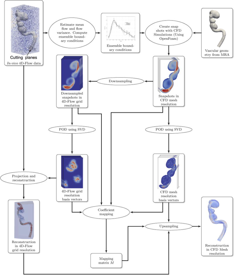
The flowchart of our algorithm is shown in Fig.1. The basic idea is to characterize the solution space of the Navier-Stokes equation in the proximity of the actual flow in terms of a POD basis followed by projection of the raw noisy 4D Flow MRI data on to this basis. This obtains the noise and divergence-free flow estimate at the 4D Flow MRI grid resolution. This is followed by a clever process of up-sampling based on a dictionary learning process (implemented using ridge regression) to obtain the flow-field at the spatial resolution of the CFD mesh.
Figure 1. Flow-chart of the hemodynamic velocity reconstruction process.
2.1. Constructing Boundary Conditions
We begin by constructing the boundary conditions (BCs) (inlet/outlet flow rate) from the actual 4D Flow MRI data. As shown in Fig. 1, the BC is estimated by placing cutting planes normal to the center line on the geometry at a number of locations (5) at the proximal (inlet) and distal (outlet) locations. The mean BC is found by averaging the results computed at various sections. The sampling rate/time resolution of 4D Flow MRI is insufficient for numerical stability of the CFD algorithm. We therefore use cubic interpolation and re-sampling to generate the BC waveform at a time resolution that enables numerical stability for the CFD solver. The sample BC standard deviation is determined and an ensemble of BCs is computed by perturbing the mean BC. The actual BC, by definition, is somewhere in the space given by the mean BC and the BC standard deviation. The ensemble BCs are used along with the vascular geometry to compute an ensemble of solutions. Time snapshots of the solutions are collected at regular simulation intervals (≈10 per 4D Flow MRI time step). These snapshots are then used to compute the proper orthogonal decomposition.
2.2. Proper Orthogonal Decomposition (POD)
POD is a method to find a set of ordered orthonormal basis vectors in a subspace where a random vector in the sample space can be expressed optimally using a linear combination of the selected first m basis vectors. In our case, the POD basis vectors span local space of all possible solutions near our ensemble of solutions. We generate our POD basis functions using the method of snapshots (Sirovich, 1987). A matrix of solutions from the ensemble of solutions is organized as:
| (2) |
where is the sequence of velocity profiles by time of the kth ensemble solution, NH is the dimension of the 3-D velocity vector in CFD mesh resolution, ND is the number of time steps for which data is collected to generate the POD basis vectors, and NQ is the number of ensemble solutions. Therefore, the total number of snapshots in [ZH] is given by Ns = ND × NQ. Consequently, . The solutions are also down-sampled to the 4D Flow MRI grid as:
| (3) |
where is the down-sampling matrix (in the current case, S computes the average of mesh finite volume center (mfvc) velocities in a 4D Flow MRI grid voxel as suggested in (Cibis et al., 2015)).
We next proceed to compute the singular value decomposition (SVD) (Golub and Reinsch, 1970) of the matrices [ZH], [ZL] as:
| (4) |
The matrices , consist of left eigenvectors, the matrix is diagonal and contains the singular values and the matrices [VH], [VL] contain the right eigenvectors. The matrices [UH], [UL] form the basis that spans the space of all possible solutions in the CFD mesh space and the down-sampled 4D Flow MRI grid space respectively.
2.3. Noise Free Reconstruction in 4D Flow MRI Grid Space
The 4D Flow MRI signal is the summation of the actual velocity and noise. While the actual velocity signal obeys the flow physics, i.e., satisfies momentum and mass conservation equations, the noise does not. Therefore, the actual velocity lies in the space of solutions spanned by the basis vectors [UL] and the noise signal is orthogonal to this space. Therefore, if we project the 4D Flow MRI data onto the basis vectors [UL], we should be able to recover the actual velocity. The projection is given by:
| (5) |
where [YL] is the 4D Flow MRI raw data. Finally, the estimate of the actual flow in the 4D Flow MRI grid is obtained as:
| (8) |
2.4. Noise Free Reconstruction at CFD Mesh Resolution Using Dictionary-based Ridge Regression
4D Flow MRI grid resolution is typically not high enough to capture the fine details of the flow-field. On the other hand, CFD can resolve these details to an arbitrarily fine level (depending on the availability of computing power, random access memory (RAM) and time). Therefore, the problem here is to find if the low resolution flow estimate can be up-sampled to the high resolution CFD mesh.
In our work, we use a dictionary learning process implemented using ridge regression for projection coefficient mapping between the low resolution space of the 4D Flow MRI grid and high resolution space of the CFD mesh. The estimate of flow velocity at the CFD mesh resolution is given by
| (7) |
To find [αH] (CFD mesh space projection coefficients), we use the relation
| (8) |
where is the mapping matrix. To obtain [M] we use ridge regression that mimimizes an objective function given by (Leyuan Fang et al., 2013; Jia et al., 2013):
| (9) |
where
| (10) |
The equations above compute the projections of the CFD mesh resolution ensemble solution snapshots and their respective down-sampled 4D Flow MRI grid resolution solution snapshots on the basis vectors. β is a regularization parameter which minimizes the effects of outliers in the data. Basically, with ridge regression, we force the matrix [M] to map known projection coefficients obtained from ensemble solutions in a least squared sense. The optimal solution is given by
| (11) |
where I is an identity matrix of size Ns × Ns.
Empirically, we have observed that choice of parameter β can impact the quality of the up-sampled solution we obtain. When is β small (10−2), up-sampled data picks up certain amount of numerical oscillations. When is β large (100) it tends to smooth out sharp features. A method to optimally determine β automatically is a problem that we will research in the near future.
2.4.1. Down-sampling CFD Results to 4D Flow MRI Grid Resolution
Down-sampling is done to compute values of the field on a regular grid from the unstructured CFD mesh. Using spatial binning, we assigned the mesh finite volume centers (mfvc) of the CFD mesh to voxels of the 4D Flow MRI grid. The velocity at the center of every voxel was then computed as the mean of all velocities of mfvc that fall within the 4D Flow MRI grid.
2.5. Numerical Phantom for Algorithm Testing
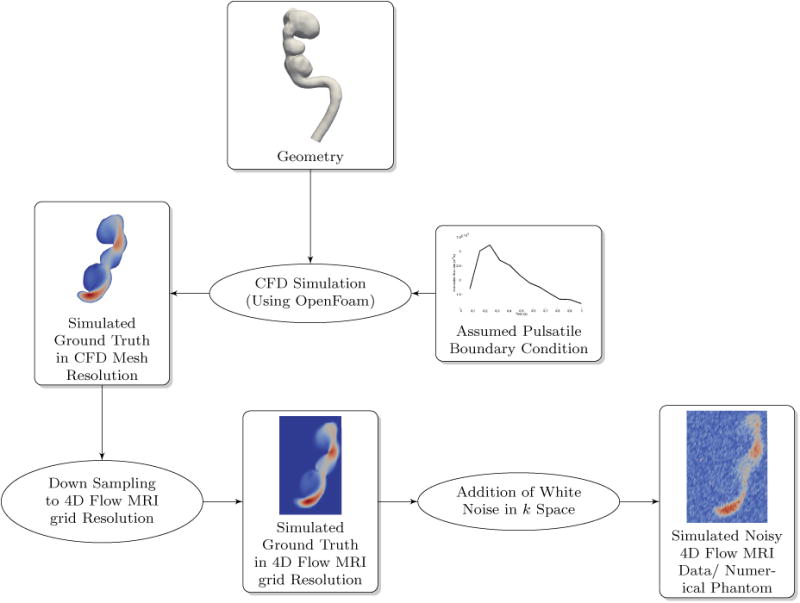
Similar to the testing methods in Ong et al. (Ong et al., 2015), we created a numerical phantom to test our algorithm. Realistic pulsatile boundary conditions along with an actual intra-cranial aneurysm geometry was used for pure CFD simulation of blood flow. The resulting velocity field was designated as the simulated ground truth. This velocity field was down-sampled to the 4D Flow MRI grid. 4D Flow MRI acquisition process was simulated by adding noise in k space to the down-sampled velocity-field (Johnson and Markl, 2010). The resulting noisy, time resolved data set was the synthetic 4D Flow MRI data set (numerical phantom) that was used to test the POD algorithm and benchmark its performance against various other de-noising methods in literature. Fig. 2 illustrates the overall process for generating the numerical phantom.
Figure 2. Creating a realistic numerical phantom for algorithm testing and comparison.
2.5.1. Patient Specific Vascular Geometry and CFD Mesh
High-resolution contrast enhanced MR angiography (CE-MRA) images were used to construct patient-specific vascular geometry. The patient was imaged at the Vascular Imaging Research Center (VIRC), University of California, San Francisco (UCSF). The voxel size in the CE-MRA images was 0.7mm × 0.7mm × 0.7 mm and the contrast ratio of the luminal to background intensity was in the range of 8 to 10. MIMICSTM (Mimics 17.0, Materialise Inc, Leuven, Belgium) was used to create a three-dimensional iso-surface corresponding to the luminal boundaries. A threshold intensity value was adjusted to ensure that the segmented iso-surface coincides with the luminal boundaries. The geometry obtained from the segmentation process included the aneurysm with its proximal and distal vessels. The iso-surface was then imported into a pre-processing software ANSYS ICEM CFD (ANSYS, Inc, Canonsburg, PA), where the computational domain and mesh were created. The computational mesh has roughly 0.6 Million finite volume cells.
2.5.2. Pulsatile Boundary Flow Conditions for the Numerical Phantom
To mimic in-vivo conditions, we sampled an in-vivo 4D Flow MRI data set as detailed in section 2.1 over the entire cardiac cycle to generate the pulsatile boundary condition wave form. The mean BC waveform thus obtained was used to generate the simulated ground truth in the CFD mesh resolution.
2.5.3. CFD Simulation
The open source software OpenFoam(Weller et al., 1998) was used to compute the CFD solutions. We used the time varying pressure implicit with splitting of operator (PISO) to integrate the discretized Navier Stokes equation. Reynold's number calculated at the inlet was estimated to be ≈ 400. At this value of Reynold's number, the flow can be assumed to be laminar (Sigovan et al., 2013). Dynamic viscosity of blood was set to 3.5 × 10⁻³Pa. Flow was assumed to be Newtonian with rigid aneurysm geometry. The time step for the PISO solver was set to 1.67ms. We are limited by the numerical stability of solver algorithm.
2.6. Error Analysis
Error metrics used for comparison between our technique and finite difference method (FDM), divergence-free radial basis functions (RBF), divergence-free wavelets with SureShrink and median absolute deviation (MAD) with and without cycle spinning (DFW-sm, DFWsms) were the same as those in (Ong et al., 2015). These include the velocity normalized root mean squared error (vNRMSE), the speed normalized root mean squared error (sNRMSE), and direction error (DE). For completeness, we include these herewith:
| (12) |
| (13) |
| (14) |
| (15) |
where N is the number of voxels within the segmented data, vi,ph is the numerical phanthom velocity in the ith voxel of the segmented data and vi,recon is the reconstructed velocity.
2.7. In-vivo 4D Flow MRI Data
4D Flow MRI flow imaging was performed on an aneurysm patient using a 3T MRI scanner (Siemens, Skyra). The number of 4D Flow MRI slices was 144 with in-plane matrix size of 194×144 pixels (voxel size of 1.25mm × 1.25mm × 1.33mm). The sequence parameters used for the MRI were as follows: TR/TE = 5.2/3.78 ms, flip angle = 8°, and temporal resolution = 83.28 ms. The VENC was set to 100cm/s. 4D Flow MRI data was imported in DICOM format to a pre-processing in-house software where the velocity data was extracted and saved for post-processing.
3. Results
3.1. Tests with Numerical Phantom
The methods developed in this work were compared to existing methods such as finite difference method (FDM), radial basis functions (RBF), and divergence free wavelets (DFW) using the numerical phantom described previously. The support of RBF basis functions was set to 7×7×7 experimentally. The number of iterations for the LSQR solver was set to be 20. The kernel size for FDM is 3×3×3 and is fixed. The minimum size for the wavelet scaling sub-band was set to 10 for both DFW-sm (with automated selection of sub-band dependent threshold using Sure-Shrink (SS) and median absolute deviation(MAD)) and DFW-sms (with SS, MAD, and partial cycle spinning). For DFW-sms, the number of spins was set to 4 which is equivalent to 16 random shifts(Ong et al., 2015). As in the case of RBF, the parameters for DFW-sm, and DFW-sms were adjusted to achieve the best error performance for the dataset.
3.1.1. Reconstruction of the Velocity Flow-Field in CFD Mesh Resolution
Fig. 3 illustrates the results of the POD reconstruction. Fig. 3(a) shows the magnitude of flow velocity of the simulated ground truth in CFD mesh resolution. Fig. 3(b) illustrates the ground truth down-sampled to the 4D Flow MRI grid resolution. As can be seen, fine features in the CFD mesh resolution are distorted just by the act of down-sampling. Therefore, it is obvious that 4D Flow MRI cannot possibly resolve fine flow features. Fig. 3(c) shows the simulated noisy 4D Flow MRI velocity magnitude after applying white noise in k space to the down-sampled ground truth. Fig. 3(d) shows the result of projecting this noisy data on to the POD basis in 4D Flow MRI grid resolution. Clearly, this result closely matches the velocity profile of the down-sampled simulated ground truth in Fig. 3(b). Fig. 3(e) illustrates the reconstruction in CFD mesh resolution after applying the ridge regression algorithm to map coefficients. As can be seen, this reconstructed result is nearly identical to the simulated ground truth in Fig. 3(a). This shows that our algorithm is able to reconstruct high resolution velocity profiles from low resolution noisy 4D Flow MRI observations with remarkable accuracy. To the best of our knowledge no other technique is able to achieve this.
Figure 3.
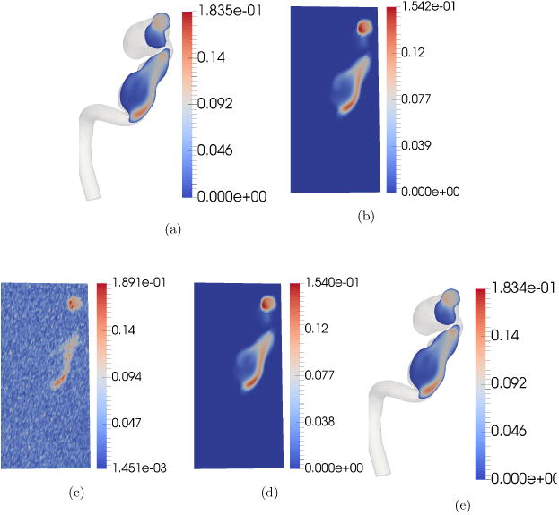
Reconstruction of velocity profile using POD. A random two dimensional cross-section was chosen for visualization purposes. The units of the color bar are in m/s. Each sub-figure shows the velocity magnitude map of the selected cross-section. (a) Simulated ground truth in CFD mesh resolution sampled at a 2-D cross-section. (b) Down-sampled simulated ground truth in 4D Flow MRI grid. (c) Simulated noisy 4D Flow MRI/Numerical Phantom after adding noise in k space. (d) De-noised velocity profile in 4D Flow MRI grid resolution. (e) Reconstructed velocity profile in CFD mesh resolution. Notice that fine details missing in the reconstructed velocity profile in the 4D Flow MRI grid resolution are revealed in the reconstructed velocity profile in CFD mesh resolution.
3.1.2. Comparison with State-of-the-art for De-noising in 4D Flow MRI Grid Resolution
Comparison tests were conducted with RBF, FDM, DFW-sm, and DFW-sms. Tests were run for two different noise levels (28.17dB PVNR corresponding to noise standard deviation of σ = 10%|vmax| and 13.2dB PVNR corresponding to noise standard deviation of σ = 50%|vmax|) at 4D Flow MRI grid resolution of 40 × 80 × 80 voxels. One additional test was run with noise standard deviation set to 50% with the 4D Flow MRI grid resolution at 21 × 51 × 25 voxels. This is the resolution of the in-vivo patient data acquisition. Each of these tests were run 20 times and the sample means and standard deviation of various error metrics were tabulated in Table 1.
Table 1.
Comparison metrics for segmented voxels with 10-50% noise level for 40 × 80 × 80 and 50% for 21×51 ×25 4D Flow MRI grid resolution respectively. These are sample mean and standard deviation of 20 trials for each comparison are listed.
| Resolution/Noise Level | Metrics/Method | Initial Noisy | FDM | RBF | DFW-sm | DFW-sms | POD |
|---|---|---|---|---|---|---|---|
| 40 × 80 × 80 10% | vNRMS | 0.039100 ± 0.000112 | 0.064865 ± 0.000075 | 0.032695 ± 0.000083 | 0.036840 ± 0.000560 | 0.029270 ± 0.000393 | 0.004590 ± 0.000055 |
| sNRMS | 0.022970 ± 0.000098 | 0.036590 ± 0.000107 | 0.022840 ± 0.000075 | 0.026980 ± 0.000605 | 0.023110 ± 0.000435 | 0.003715 ± 0.000049 | |
| DE | 0.057935 ± 0.000723 | 0.073955 ± 0.000793 | 0.038520 ± 0.000801 | 0.024470 ± 0.000511 | 0.012370 ± 0.000508 | 0.000185 ± 0.000037 | |
| 20% | vNRMS | 0.078755 ± 0.000221 | 0.085045 ± 0.000154 | 0.046730 ± 0.000184 | 0.058575 ± 0.001114 | 0.045880 ± 0.000620 | 0.005915 ± 0.000169 |
| sNRMS | 0.047560 ± 0.000233 | 0.048730 ± 0.000117 | 0.030500 ± 0.000172 | 0.044085 ± 0.001375 | 0.037410 ± 0.000723 | 0.004800 ± 0.000130 | |
| DE | 0.117110 ± 0.000772 | 0.114755 ± 0.000832 | 0.066040 ± 0.000971 | 0.043105 ± 0.002119 | 0.021405 ± 0.000610 | 0.000260 ± 0.000050 | |
| 30% | vNRMS | 0.120120 ± 0.000401 | 0.112140 ± 0.000310 | 0.065615 ± 0.000322 | 0.075890 ± 0.000744 | 0.059255 ± 0.000774 | 0.007715 ± 0.000272 |
| sNRMS | 0.074495 ± 0.000338 | 0.065800 ± 0.000367 | 0.041915 ± 0.000328 | 0.057570 ± 0.001213 | 0.049115 ± 0.000921 | 0.006245 ± 0.000211 | |
| DE | 0.171225 ± 0.001349 | 0.157620 ± 0.001162 | 0.095495 ± 0.001266 | 0.059875 ± 0.002764 | 0.029335 ± 0.001492 | 0.000430 ± 0.000057 | |
| 40% | vNRMS | 0.164840 ± 0.000596 | 0.144370 ± 0.000555 | 0.088170 ± 0.000359 | 0.091715 ± 0.001070 | 0.070835 ± 0.000624 | 0.009965 ± 0.000365 |
| sNRMS | 0.105305 ± 0.000450 | 0.086980 ± 0.000350 | 0.056735 ± 0.000375 | 0.068920 ± 0.001000 | 0.059050 ± 0.000871 | 0.008065 ± 0.000331 | |
| DE | 0.218580 ± 0.001800 | 0.199195 ± 0.001220 | 0.125245 ± 0.001458 | 0.079265 ± 0.003582 | 0.037845 ± 0.001595 | 0.000730 ± 0.000098 | |
| 50% | vNRMS | 0.216380 ± 0.000888 | 0.183390 ± 0.000863 | 0.114670 ± 0.000728 | 0.108770 ± 0.002401 | 0.082435 ± 0.000775 | 0.012835 ± 0.000660 |
| sNRMS | 0.142665 ± 0.000604 | 0.113515 ± 0.000704 | 0.074955 ± 0.000691 | 0.080960 ± 0.001491 | 0.068160 ± 0.001117 | 0.010395 ± 0.000544 | |
| DE | 0.259455 ± 0.001487 | 0.238690 ± 0.001684 | 0.156835 ± 0.001717 | 0.100970 ± 0.007125 | 0.049930 ± 0.002881 | 0.001185 ± 0.000150 | |
| 21 × 51 × 25 50% | vNRMS | 0.217025 ± 0.002955 | 0.181650 ± 0.002163 | 0.129055 ± 0.002100 | 0.127545 ± 0.002768 | 0.092225 ± 0.001404 | 0.032320 ± 0.001784 |
| sNRMS | 0.143245 ± 0.002402 | 0.112725 ± 0.001885 | 0.085240 ± 0.001918 | 0.085915 ± 0.001730 | 0.064945 ± 0.001425 | 0.024830 ± 0.001300 | |
| DE | 0.256875 ± 0.003177 | 0.234325 ± 0.003102 | 0.168690 ± 0.003423 | 0.146700 ± 0.008493 | 0.095905 ± 0.004848 | 0.013465 ± 0.002194 |
As can be seen from Fig.4, for 10% noise level and 4D Flow MRI grid resolution of 40 × 80 × 80 voxels, for all methods, the visual quality is almost the same. The overall quantitative error metrics shown in Table 1 indicate that in order of performance, FDM performs the worst (it actually amplifies noise), DFW-sm is next, followed by RBF, DFW-sms, and POD. As can be seen, the second best technique DFW-sms has about 6.127×, 6.22×, and 66.86× the vNRMS, sNRMS, and DR error of POD. However, the performance degrades with higher noise. The error metrics in Table 1 indicate that by order of performance, FDM performs the worst, RBF is next, followed by DFW-sm, DFW-sms, and POD. In this case, the second best method DFW-sms has about 6.42×, 6.55×, and 42.135× the vNRMS, sNRMS, and DR error of POD.
Figure 4.
De-noising comparison on simulated data. The units of the color bar are in m/s. In this test, the noise standard deviation was set to be σ = 10%|Vmax |. The 4D Flow MRI grid resolution was set to 40 × 80 × 80 voxels. (a) 2-D section location for sampling velocity. (b) Down-sampled ground truth at the 2-D section. (c) Simulated noisy 4D Flow MRI. (d) De-noising using FDM. (e) De-noising using RBF. (f) De-noising using DFM-sm. (g) De-noising using DFM-sms. (h) De-noising using POD. All methods visually appear to more or less preserve details in the velocity profile.
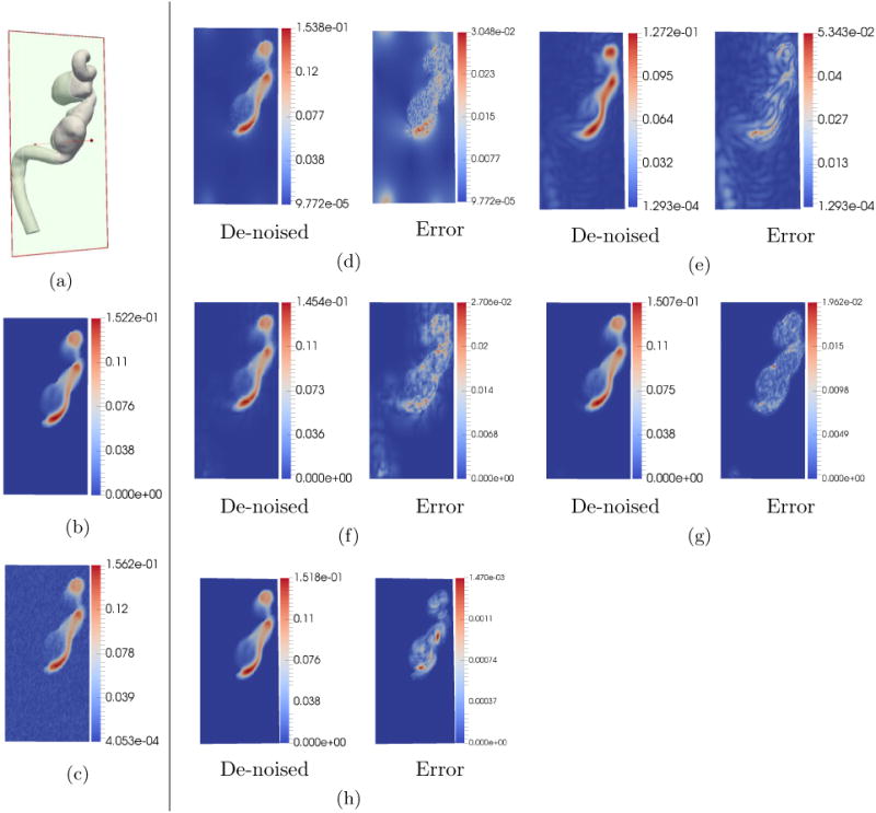
Fig. 5 illustrates the results of tests when noise was set to 50% with reduced 4D Flow MRI grid resolution of 21×51×25 voxels (resolution of in-vivo data). As can be seen, previous de-noising techniques have significant distortion in velocity patterns. POD reconstruction works much better as shown in Fig.5(e).
Figure 5.
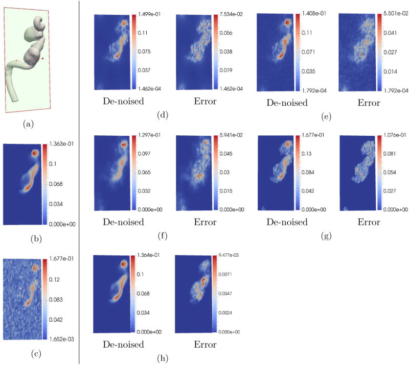
De-noising comparison on simulated data with high noise and low 4D Flow MRI grid resolution. The units of the color bar are in m/s. In this test, the noise standard deviation was set to be σ = 50%|Vmax |. The 4D Flow MRI grid resolution was set to 21 × 51 × 25 voxels which is the same for in-vivo 4D Flow MRI. (a) 2D section at which velocity magnitudes were sampled. (b) Down-sampled ground truth. (c) Simulated noisy 4D Flow MRI. (d) De-noising using FDM. (e) De-noising using RBF. (f) De-noising using DFW-sm. (g) Reconstruction using DFW-sms. (h) De-noising using POD. Clearly, as can be seen in the figure, POD method is able to preserve details in the flow much better than all other methods.
Fig. 6 illustrates the velocity magnitudes at 2 1-D cross sections as shown in Fig. 6(b). Results for 10% noise level indicate all previous methods work reasonably well (Fig. 6 (c),(d)). POD seems to have the least distortion. For the 50% noise level, DFW-sms and DFW-sm seem to have surprisingly large amount of distortion as indicated in Fig.6(f). POD on the other hand is able to recover the velocity profile significantly better (Fig.6(g)).
Figure 6.
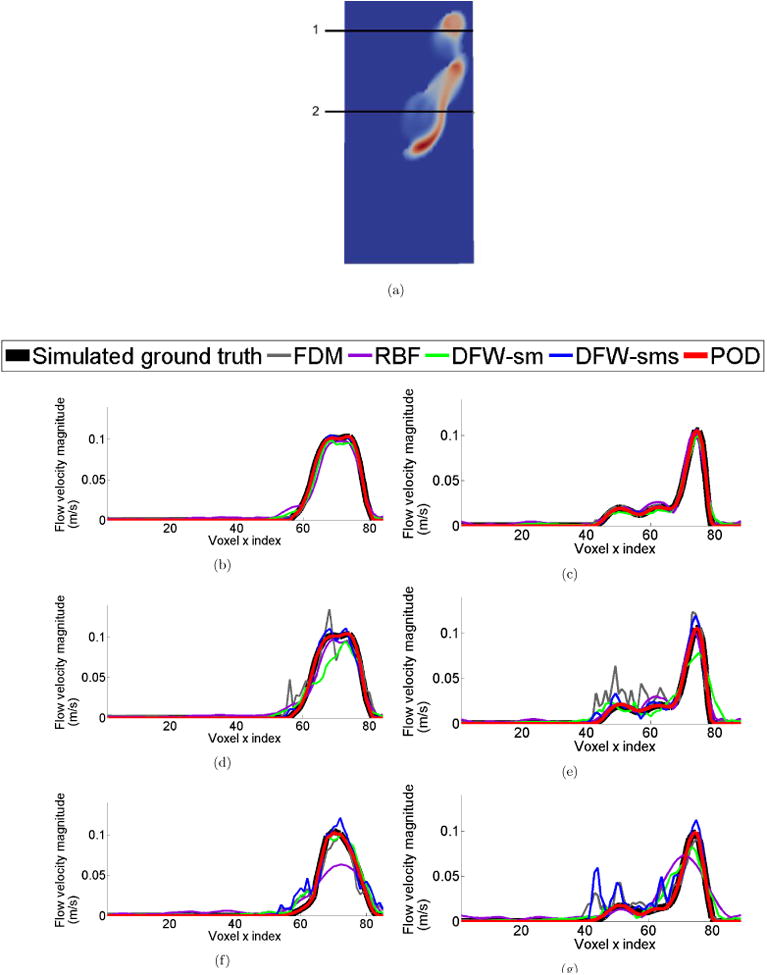
Comparison of velocity profiles along 1-D sections. (a) Location of sampled 1-D sections. (b), (c) Velocity profile comparison when noise standard deviation was set to be σ = 10%|Vmax | at 1-D sections ‘1’ and ‘2’ respectively with resolution of 40 × 80 × 80 voxels. (d),(e) Velocity profile comparison when noise standard deviation was set to be σ = 50%|Vmax | at 1-D sections ‘1’ and ‘2’ respectively with resolution of 40 × 80 × 80 voxels. And (f),(g) Velocity profile comparison when noise standard deviation was set to be σ = 50%|Vmax | at 1-D sections ‘1’ and ‘2’ respectively with resolution of 21 × 51 × 25 voxels. Clearly, POD performs much better than all other methods. There is significant degradation in the results of other methods when noise level is increased.
3.1.3. Sensitivity Analysis
We varied the number of ensemble solutions NQ used to generate the POD basis, to test the sensitivity of the reconstructed results to NQ. Fig. 7 (a) shows the velocity magnitude at a particular 2-D section of the down-sampled ground truth. Fig. 7(b) - (e) shows the reconstructed results by using POD basis obtained from NQ = 6, 5, 4, 3, respectively. In each of these trials, we made sure that one of the solutions used to generate the POD basis was generated using the mean boundary condition obtained from sampling the simulated noisy 4D Flow MRI data set. It can clearly be seen that magnitude plots are almost identical (within 4 × 10⁻³) to the ground truth. It appears that the results are relatively robust to change in NQ.
Figure 7.

Sensitivity Analysis. The units of the color bar are in m/s. Here we check the sensitivity of the reconstructed results to changing NQ, the number of ensemble solutions used to generate solutions to construct the POD basis.Image (a) is the simulated down-sampled ground truth, (b)-(e) are results from setting NQ = 6, 5, 4, 3 respectively. In each trial, the mean flow (boundary condition) computed from sampling the simulated noise 4D Flow MRI data is part of the ensemble used to compute the POD basis.
3.2. Tests on in-vivo Data
We also tested our algorithm on in-vivo data.(Fig. 8). In this case, the ground truth is not available. Fig. 8 (d), (e) show the results of our de-noising with reconstruction at CFD mesh resolution and streamlines respectively. We then compared our results against reconstruction using DFW (Fig. 9). As in (Ong et al., 2015), we performed streamline tests. Streamlines were constructed from the velocity data for the raw 4D Flow MRI data, reconstruction with DFW, and reconstruction with POD in 4D Flow MRI mesh resolution. We used the ParaView software to build streamlines from velocity data. Significant manual adjustment of parameters (threshold, sub band level etc.) with DFW had to be performed to generate results. DFM-sms failed to produce any coherent results. An emitter plane was place near the inlet and an analysis plane was placed near the outlet. Since this aneurysm has only one inlet and one outlet, it can be assumed that all streamlines released at the emitter should reach the analysis plane. In case of DFW, only 7.3 % of the streamlines reached the analysis plane. For POD-based de-noising in 4D Flow MRI resolution, 87.8 % reached the analysis plane. For comparison, in case of the raw 4D Flow MRI data, only 1% reached the analysis plane. Clearly, the POD approach greatly improves streamline lengths.
Figure 8.
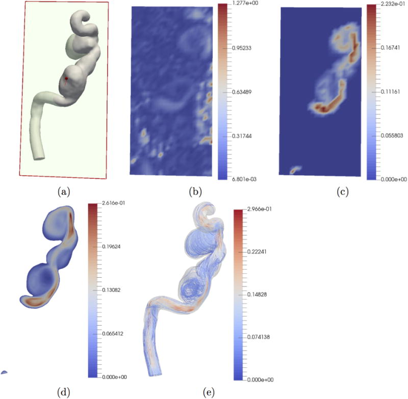
De-noising and reconstruction from in-vivo data. The units of the color bar are in m/s. (a) 2-D section at which results are displayed. (b) Raw in-vivo 4D Flow MRI data. (c) POD-based de-noising in 4D Flow MRI grid resolution. (d) POD-based reconstruction using ridge regression in CFD mesh resolution. (e) Streamlines of CFD mesh resolution reconstruction.
Figure 9.
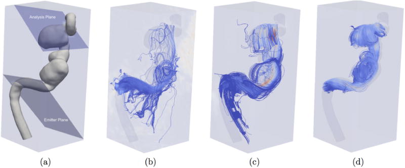
Comparison of de-noising on in-vivo 4D Flow MRI data using streamlines. (a) Location of emitter and analysis planes. (b) Unprocessed in-vivo 4D Flow MRI streamlines. (c) DFW streamlines (with manual optimization of parameters for the algorithm). (d) POD streamlines.
4. Discussion
A new method based on proper orthogonal decomposition for reconstructing high resolution hemodynamic velocity profiles from low resolution noisy time resolved phase contrast magnetic resonance was developed. Furthermore, a novel technique based on ridge regression was developed for up-sampling of the results from the 4D Flow MRI grid to the unstructured high resolution CFD mesh. The performance of the proposed techniques was tested against existing techniques such as FDM, RBF, and DFW using a numerical phantom. Since our techniques use actual CFD simulation to generate basis vectors, unlike most of the previous methods, our solutions conform to both the momentum balance as well as mass balance parts of the Navier-Stokes equation. The ability to up-sample means that our technique can be used to potentially recover minute flow details that are not visible at the resolution of 4D Flow MRI acquisition. Alternatively, our technique can be used in situations where size of the blood vessels in question limits the resolution of the 4D Flow MRI acquisition.
In our work we have assumed laminar Newtonian flow model in the CFD simulation based on the Reynold's number. However, non-Newtonian flow models can easily be incorporated without any change in the basic process. Uncertainty in the viscosities and other parameters can be handled by process of sampling which will increase the number of CFD solutions used to generate the basis vectors.
Tuning of the parameters plays a significant role in the performance of the techniques used for de-noising of 4D Flow MRI data. While FDM has no parameters (it is based on a fixed 3×3 kernel), RBF requires specification of radius r for its kernel and the max. number of iterations for its LSQR solver. For DFW-sm the user should specify the minimum size of wavelet scaling sub-bands. For DFW-sms, the number of cycle spins should also be specified. Our algorithm requires the specification of the parameter β in ridge regression. In the current work, it was chosen experimentally based on the quantitative measures when comparing with the simulated ground truth data.
Currently, a major limitation of our technique is computational complexity. Several CFD simulations (ensemble) have to be carried out to generate the POD basis. The high fidelity patient specific CFD mesh, in our tests, has approximately 600,000 nodes. On an AMD Phenom II X4 920 Processor computer with 16 GB of RAM in Ubuntu 14.04 LTS environment with OpenFOAM 3.0 without any multi-core modifications took around 10 hours per simulation. We then used a parallel implementation on Google Cloud which brought down the total simulation time for 6 ensembles to 1hr. Currently, we use an explicit time solver and are limited by the numerical stability of the integrator. Using a fully implicit block coupled solver (Darwish and Moukalled, 2014) may significantly reduce the computation time. Furthermore, sensitivity analysis shows that the results do not change appreciably with the number of ensembles (Fig. 7). Based on this result, in our following publication, we will test our technique with NQ = 1 on an intra-cranial aneurysm geometry with multiple inlets and outlets.
Finally, the proposed method has been tested on only a single intra-cranial aneurysm geometry. In the near future, we plan to run in-silico validation tests on multiple geometries. Also lacking is an in-vitro test where our method will be tested against a method such as particle image velocimetry (PIV) which has a much higher resolution as compared to 4D Flow MRI. We are working with our collaborators on building and testing an in-vitro model. The results will be presented in a subsequent paper.
5. Conclusion
A novel technique based on proper orthogonal decomposition and ridge regression for detailed reconstruction of hemodynamic velocity profiles at arbitrary levels of detail from low resolution noisy phase contrast magnetic resonance (4D Flow MRI) data has been developed. Benchmark tests indicated this technique performs better in de-noising and at the same time preserving details in the velocity profiles. Furthermore, our technique merges patient-specific CFD simulation with 4D Flow MRI observations and is able to recover the underlying velocity profiles at arbitrarily higher spatial resolutions. Therefore, this technique may improve the ability to accurately derive clinically relevant secondary parameters such as wall shear stresses and pressure gradients at a much higher level of detail and confidence than was previously possible.
Acknowledgments
This work was partly supported by grant NIH HL115267 from the National Institute of Health. The content is solely the responsibility of the authors and does not necessarily represent the official views of the National Institutes of Health. We thank the reviewers for insightful comments that have helped us to greatly improve this paper.
Footnotes
Conflict of interest statement: The authors declare that they have no conflict of interest.
Publisher's Disclaimer: This is a PDF file of an unedited manuscript that has been accepted for publication. As a service to our customers we are providing this early version of the manuscript. The manuscript will undergo copyediting, typesetting, and review of the resulting proof before it is published in its final citable form. Please note that during the production process errors may be discovered which could affect the content, and all legal disclaimers that apply to the journal pertain.
References
- Bostan E, Lefkimmiatis S, Vardoulis O, Stergiopulos N, Unser M. Improved variational denoising of flow fields with application to phase-contrast mri data. Signal Processing Letters, IEEE. 2015a;22(6):762–766. [Google Scholar]
- Bostan E, Unser M, Ward JP. Divergence-Free Wavelet Frames. IEEE Signal Processing Letters. 2015b Aug;22(8):1142–1146. URL http://ieeexplore.ieee.org/document/7001623/ [Google Scholar]
- Boussel L, Rayz V, Martin A, Acevedo-Bolton G, Lawton MT, Higashida R, Smith WS, Young WL, Saloner D. Phase-contrast magnetic resonance imaging measurements in intracranial aneurysms in vivo of flow patterns, velocity fields, and wall shear stress: comparison with computational fluid dynamics. Magnetic Resonance in Medicine. 2009;61(2):409–417. doi: 10.1002/mrm.21861. [DOI] [PMC free article] [PubMed] [Google Scholar]
- Busch J, Giese D, Wissmann L, Kozerke S. Reconstruction of divergence-free velocity fields from cine 3D phase-contrast flow measurements. Magnetic resonance in medicine. 2013;69(1):200–210. doi: 10.1002/mrm.24221. [DOI] [PubMed] [Google Scholar]
- Cibis M, Jarvis K, Markl M, Rose M, Rigsby C, Barker AJ, Wentzel JJ. The effect of resolution on viscous dissipation measured with 4d flow mri in patients with fontan circulation: Evaluation using computational fluid dynamics. Journal of biomechanics. 2015;48(12):2984–2989. doi: 10.1016/j.jbiomech.2015.07.039. [DOI] [PMC free article] [PubMed] [Google Scholar]
- Darwish M, Moukalled F. A fully coupled navier-stokes solver for fluid flow at all speeds. Numerical Heat Transfer Part B: Fundamentals. 2014;65(5):410–444. [Google Scholar]
- Deriaz E, Perrier V. Divergence-free and curl-free wavelets in two dimensions and three dimensions: application to turbulent flows. Journal of Turbulence. 2006 Jan;7:N3. URL http://www.tandfonline.com/doi/abs/10.1080/14685240500260547. [Google Scholar]
- Donati F, Figueroa CA, Smith NP, Lamata P, Nordsletten DA. Non-invasive pressure difference estimation from pc-mri using the work-energy equation. Medical image analysis. 2015;26(1):159–172. doi: 10.1016/j.media.2015.08.012. [DOI] [PMC free article] [PubMed] [Google Scholar]
- Ebbers T, Wigstrom L, Bolger A, Wranne B, Karlsson M. Noninvasive measurement of time-varying three-dimensional relative pressure fields within the human heart. Journal of biomechanical engineering. 2002;124(3):288–293. doi: 10.1115/1.1468866. [DOI] [PubMed] [Google Scholar]
- Fang L, Li S, McNabb RP, Nie Q, Kuo AN, Toth CA, Izatt JA, Farsiu S. Fast acquisition and reconstruction of optical coherence tomography images via sparse representation. IEEE transactions on medical imaging. 2013 Nov;32(11):2034–49. doi: 10.1109/TMI.2013.2271904. [DOI] [PMC free article] [PubMed] [Google Scholar]
- Ferziger JH, Perić M. Computational Methods for Fluid Dynamics. Springer Berlin Heidelberg; Berlin, Heidelberg: 2002. URL http://link.springer.com/10.1007/978-3-642-56026-2. [Google Scholar]
- Golub GH, Reinsch C. Singular value decomposition and least squares solutions. Numerische mathematik. 1970;14(5):403–420. [Google Scholar]
- Harloff A, Nuβbaumer A, Bauer S, Stalder AF, Frydrychowicz A, Weiller C, Hennig J, Markl M. In vivo assessment of wall shear stress in the atherosclerotic aorta using flow-sensitive 4d mri. Magnetic resonance in medicine. 2010;63(6):1529–1536. doi: 10.1002/mrm.22383. [DOI] [PubMed] [Google Scholar]
- Huang F, Akao J, Vijayakumar S, Duensing GR, Limkeman M. k-t grappa: A k-space implementation for dynamic mri with high reduction factor. Magnetic resonance in medicine. 2005;54(5):1172–1184. doi: 10.1002/mrm.20641. [DOI] [PubMed] [Google Scholar]
- Jang D, Jetli R, Acharya S. Comparison of the piso, simpler, and simplec algorithms for the treatment of the pressure-velocity coupling in steady flow problems. Numerical Heat Transfer Part A: Applications. 1986;10(3):209–228. [Google Scholar]
- Jia K, Wang X, Tang X. Image Transformation Based on Learning Dictionaries across Image Spaces. IEEE Transactions on Pattern Analysis and Machine Intelligence. 2013 Feb;35(2):367–380. doi: 10.1109/TPAMI.2012.95. URL http://ieeexplore.ieee.org/document/6189355/ [DOI] [PubMed] [Google Scholar]
- Johnson KM, Markl M. Improved snr in phase contrast velocimetry with five-point balanced flow encoding. Magnetic resonance in medicine. 2010;63(2):349–355. doi: 10.1002/mrm.22202. [DOI] [PMC free article] [PubMed] [Google Scholar]
- Johnston BM, Johnston PR, Corney S, Kilpatrick D. Non-newtonian blood flow in human right coronary arteries: steady state simulations. Journal of biomechanics. 2004;37(5):709–720. doi: 10.1016/j.jbiomech.2003.09.016. [DOI] [PubMed] [Google Scholar]
- Karhunen K. Über lineare Methoden in der Wahrscheinlichkeitsrechnung. Vol. 37. Universitat Helsinki; 1947. [Google Scholar]
- Karmonik C, Klucznik R, Benndorf G. Comparison of velocity patterns in an acoma aneurysm measured with 2d phase contrast mri and simulated with cfd. Technology and Health Care. 2008;16(2):119–128. [PubMed] [Google Scholar]
- Kerschen G, Golinval Jc, Vakakis AF, Bergman LA. The method of proper orthogonal decomposition for dynamical characterization and order reduction of mechanical systems: an overview. Nonlinear dynamics. 2005;41(1-3):147–169. [Google Scholar]
- Kosambi D. Statistics in function space. J Indian Math Soc. 1943;7(1):76–88. [Google Scholar]
- Ku DN. Blood flow in arteries. Annual Review of Fluid Mechanics. 1997;29(1):399–434. [Google Scholar]
- Ku DN, Giddens DP, Zarins CK, Glagov S. Pulsatile flow and atherosclerosis in the human carotid bifurcation. positive correlation between plaque location and low oscillating shear stress. Arteriosclerosis, thrombosis, and vascular biology. 1985;5(3):293–302. doi: 10.1161/01.atv.5.3.293. [DOI] [PubMed] [Google Scholar]
- Leyuan Fang ShutaoLi, McNabb RP, Qing Nie, Kuo AN, Toth CA, Izatt JA, Farsiu S. Fast Acquisition and Reconstruction of Optical Coherence Tomography Images via Sparse Representation. IEEE Transactions on Medical Imaging. 2013 Nov;32(11):2034–2049. doi: 10.1109/TMI.2013.2271904. URL http://ieeexplore.ieee.org/document/6553142/ [DOI] [PMC free article] [PubMed] [Google Scholar]
- Loeve M. Fonctions aléatoires du second ordre. In: Levy P, editor. Processus stochastiques et mouvement Brownien. Gauthier-Villars: 1948. [Google Scholar]
- Lustig M, Pauly JM. Spirit: Iterative self-consistent parallel imaging reconstruction from arbitrary k-space. Magnetic Resonance in Medicine. 2010;64(2):457–471. doi: 10.1002/mrm.22428. [DOI] [PMC free article] [PubMed] [Google Scholar]
- Lustig M, Santos JM, Donoho DL, Pauly JM. kt sparse: High frame rate dynamic mri exploiting spatio-temporal sparsity. Proceedings of the 13th Annual Meeting of ISMRM; Seattle. 2006. [Google Scholar]
- Markl M, Chan FP, Alley MT, Wedding KL, Draney MT, Elkins CJ, Parker DW, Wicker R, Taylor CA, Herfkens RJ, et al. Time-resolved three-dimensional phase-contrast mri. Journal of Magnetic Resonance Imaging. 2003;17(4):499–506. doi: 10.1002/jmri.10272. [DOI] [PubMed] [Google Scholar]
- Milner JS, Moore JA, Rutt BK, Steinman DA. Hemodynamics of human carotid artery bifurcations: computational studies with models reconstructed from magnetic resonance imaging of normal subjects. Journal of vascular surgery. 1998;28(1):143–156. doi: 10.1016/s0741-5214(98)70210-1. [DOI] [PubMed] [Google Scholar]
- Moore J, Steinman D, Holdsworth D, Ethier C. Accuracy of computational hemodynamics in complex arterial geometries reconstructed from magnetic resonance imaging. Annals of biomedical engineering. 1999;27(1):32–41. doi: 10.1114/1.163. [DOI] [PubMed] [Google Scholar]
- Moyle KR, Antiga L, Steinman DA. Inlet conditions for image-based cfd models of the carotid bifurcation: is it reasonable to assume fully developed flow? Journal of biomechanical engineering. 2006;128(3):371–379. doi: 10.1115/1.2187035. [DOI] [PubMed] [Google Scholar]
- Nayak KS, Nielsen JF, Bernstein MA, Markl M, Gatehouse PD, Botnar RM, Saloner D, Lorenz C, Wen H, Hu BS, et al. Cardiovascular magnetic resonance phase contrast imaging. Journal of Cardiovascular Magnetic Resonance. 2015;17(1):1–26. doi: 10.1186/s12968-015-0172-7. [DOI] [PMC free article] [PubMed] [Google Scholar]
- Ong F, Uecker M, Tariq U, Hsiao A, Alley MT, Vasanawala SS, Lustig M. Robust 4D flow denoising using divergence-free wavelet transform. Magnetic resonance in medicine. 2015 Feb;73(2):828–42. doi: 10.1002/mrm.25176. [DOI] [PMC free article] [PubMed] [Google Scholar]
- Pedersen H, Kozerke S, Ringgaard S, Nehrke K, Kim WY. k-t pca: Temporally constrained k-t blast reconstruction using principal component analysis. Magnetic resonance in medicine. 2009;62(3):706–716. doi: 10.1002/mrm.22052. [DOI] [PubMed] [Google Scholar]
- Pelc NJ, Herfkens RJ, Shimakawa A, Enzmann DR. Phase contrast cine magnetic resonance imaging. Magnetic resonance quarterly. 1991;7(4):229–254. [PubMed] [Google Scholar]
- Rayz VL, Boussel L, Acevedo-Bolton G, Martin AJ, Young WL, Lawton MT, Higashida R, Saloner D. Numerical simulations of flow in cerebral aneurysms: comparison of cfd results and in vivo mri measurements. Journal of biomechanical engineering. 2008;130(5):051011. doi: 10.1115/1.2970056. [DOI] [PubMed] [Google Scholar]
- Rispoli VC, Nielsen JF, Nayak KS, Carvalho JL. Computational fluid dynamics simulations of blood flow regularized by 3d phase contrast mri. Biomedical engineering online. 2015;14(1):110. doi: 10.1186/s12938-015-0104-7. [DOI] [PMC free article] [PubMed] [Google Scholar]
- Shahcheraghi N, Dwyer H, Cheer A, Barakat A, Rutaganira T. Unsteady and three-dimensional simulation of blood flow in the human aortic arch. Journal of biomechanical engineering. 2002;124(4):378–387. doi: 10.1115/1.1487357. [DOI] [PubMed] [Google Scholar]
- Sigovan M, Rayz V, Gasper W, Alley HF, Owens CD, Saloner D. Vascular remodeling in autogenous arterio-venous fistulas by mri and cfd. Annals of biomedical engineering. 2013;41(4):657–668. doi: 10.1007/s10439-012-0703-4. [DOI] [PMC free article] [PubMed] [Google Scholar]
- Sirovich L. Method of snapshots. Q Appl Math. 1987;45:561–571. [Google Scholar]
- Song SM, Napel S, Glover GH, Pelc NJ. Noise reduction in three-dimensional phase-contrast MR velocity measurementsl. Journal of Magnetic Resonance Imaging. 1993;3(4):587–596. doi: 10.1002/jmri.1880030407. [DOI] [PubMed] [Google Scholar]
- Stalder A, Russe M, Frydrychowicz A, Bock J, Hennig J, Markl M. Quantitative 2d and 3d phase contrast mri: optimized analysis of blood flow and vessel wall parameters. Magnetic resonance in medicine. 2008;60(5):1218–1231. doi: 10.1002/mrm.21778. [DOI] [PubMed] [Google Scholar]
- Steinman DA, Taylor CA. Flow imaging and computing: large artery hemodynamics. Annals of biomedical engineering. 2005;33(12):1704–1709. doi: 10.1007/s10439-005-8772-2. [DOI] [PubMed] [Google Scholar]
- Tafti PD, Delgado-Gonzalo R, Stalder AF, Unser M. Biomedical Imaging: From Nano to Macro, 2011 IEEE International Symposium on. IEEE; 2011. Variational enhancement and denoising of flow field images; pp. 1061–1064. [Google Scholar]
- Tikhonov AN, Goncharsky A, Stepanov V, Yagola AG. Numerical methods for the solution of ill-posed problems. Vol. 328. Springer Science & Business Media; 2013. [Google Scholar]
- Tsao J, Boesiger P, Pruessmann KP. k-t blast and k-t sense: Dynamic mri with high frame rate exploiting spatiotemporal correlations. Magnetic Resonance in Medicine. 2003;50(5):1031–1042. doi: 10.1002/mrm.10611. [DOI] [PubMed] [Google Scholar]
- Vali A, Abla AA, Lawton MT, Saloner D, Rayz VL. Computational Fluid Dynamics modeling of contrast transport in basilar aneurysms following flow-altering surgeries. Journal of Biomechanics. 2017 Jan;50:195–201. doi: 10.1016/j.jbiomech.2016.11.028. URL http://linkinghub.elsevier.com/retrieve/pii/S002192901631199X. [DOI] [PMC free article] [PubMed] [Google Scholar]
- Wake AK, Oshinski JN, Tannenbaum AR, Giddens DP. Choice of in vivo versus idealized velocity boundary conditions influences physiologically relevant flow patterns in a subject-specific simulation of flow in the human carotid bifurcation. Journal of biomechanical engineering. 2009;131(2):021013. doi: 10.1115/1.3005157. [DOI] [PMC free article] [PubMed] [Google Scholar]
- Weller HG, Tabor G, Jasak H, Fureby C. A tensorial approach to computational continuum mechanics using object-oriented techniques. Computers in Physics. 1998 Nov;12(6):620. [Google Scholar]


