A design for phase I trials in completely or partially ordered groups

Abstract

We propose a design for dose finding for cytotoxic agents in completely or partially ordered groups of patients. By completely ordered groups, we mean that prior to the study, there is clinical information that would indicate that for a given dose, the groups can be ordered with respect to the probability of toxicity at that dose. With partially ordered groups, at a given dose, only some of the groups can be ordered with respect to the probability of toxicity at that dose. The method we propose includes elements of the parametric model used in the continual reassessment method combined with the Hwang-Peddada order-restricted estimation procedure. We evaluate the operating characteristics of these designs in a family of dose–toxicity curves representing complete and partial orders.

1. Background

It is becoming more common in oncology research to conduct dose-finding trials that estimate a maximum tolerated dose (MTD) of a cytotoxic agent in each of several heterogeneous groups of patients. By definition, the MTD is the highest dose that can be administered with an ‘acceptable level’ of toxicity. In this situation, ‘acceptable’ means limiting the proportion of patients who experience a sufficiently severe, protocol-specified adverse event, usually called a ‘dose-limiting toxicity’ (DLT). With cytotoxic agents, it is generally assumed that the greater the dose administered, the greater the probability that a patient will experience a DLT.

Examples of such trials include Ramanathan et al. [1] and LoRusso et al. [2], who stratify patients into ‘none’, ‘mild’, ‘moderate’, or ‘severe’ liver dysfunction at baseline. Leal et al. [3] divide patients into groups defined by increasing renal dysfunction at baseline based on a measure of 24-h creatinine clearance. Kim et al. [4] genotyped UGT1A1*28 and *6 and defined patient cohorts by the number of defective alleles: 0, 1, or 2. Satoh et al. [5] also investigated dose fining with groups defined by UGT1A1 genotypes. In this study, patients were divided into three groups according to wild-type (*1*1), heterozygous (*28*1 and *6*1), or homozygous (*28*28, *6*6, and *28*6). Each of these studies is an example of ‘completely ordered’ groups. For a given dose of the agent, we would anticipate a greater chance that a patient with a greater degree of organ dysfunction at baseline or a greater number of defective alleles would experience a DLT.

Innocenti et al. [6] provide an example of a trial conducted in partially ordered groups. Based on the observation that the risk of severe neutropenia with irinotecan is related in part to UGT1A1*28, the study sought to identify the MTD of irinotecan in patients with advanced solid tumors stratified by the *1/*1, *1/*28, and *28/*28 genotypes. The greatest risk of a DLT was expected to be in patients with the *28/*28 genotype.

Partially ordered groups can also arise naturally in classifications based on two or more stratification factors. For example, in the Satoh study, it is possible to imagine that patients in the heterozygous (*28*1 and *6*1) could be further subdivided into separate cohorts (*28*1) and (*6*1). In this case, there would be a partial order in that patients in each of these groups would be expected to have a greater risk of a DLT than patients in the wild-type group and less risk of a DLT than patients in the homozygous (*28*28, *6*6, and *28*6) group, but it might not be known prior to the study which of the groups (*28*1) or (*6*1) would have the greater toxicity.

These trials [1–5] differed in how the groups of patients are defined and what was known about the groups in terms of the risk of a DLT, but they shared the common feature that the MTD in each group was determined only from the data obtained within that patient group. In general, ignoring the group structure can lead to at least two problems: reversals and inefficiency. By reversals, we mean that the MTDs in the groups can contradict what is known clinically. For example, conducting separate trials within each group might recommend a greater dose level as the MTD in the most severely impaired group compared with a less severely impaired group. By inefficiency, we mean that a design that takes into account the known clinical relationship might recommend the correct MTDs in the groups a greater proportion of times.

In many ways, dose finding in heterogeneous groups resembles dose finding for combinations of cytotoxic agents but there are important differences. Several dose-finding methods in combination agent studies attempt to find a single MTD [7–9], while in the heterogeneous groups case, the goal is to provide an estimate of the MTD in each of the groups. While other combination methods [10, 11] target multiple MTDs, combination agent studies and those in heterogeneous groups of patients differ in how patients can be allocated. With combinations, the investigator can assign the dose of both agents to patients; in studies with heterogeneous groups, the group assignment is a characteristic of the patient and not under the control of the investigator.

1.1. Previously proposed methods for heterogeneous groups

Several methods have been proposed for dose finding in two groups of patients. O’Quigley et al. [12] introduced a two-sample continual reassessment method (CRM), which allowed for the identification of the appropriate MTD’s for two groups simultaneously. Legedza and Ibrahim [13] proposed a related method, augmenting the dose–toxicity model for a vector of patient characteristics and putting a prior on the coefficient in the dose–toxicity model. O’Quigley and Paoletti [14] proposed a two-parameter CRM for ordered groups that utilizes known differences between the groups. Ivanova and Wang [15] also incorporate isotonic estimates into designs for ordered groups that take into account both toxicity and efficacy endpoints. Wages et al. [16] describe the design of a dose-finding trial that explicitly uses the known ordering in the probabilities associated with ‘good’ and ‘poor’ prognosis patients. Their design is based on the shift model [17–19] that generalizes the CRM to two ordered groups. Conaway and Wages [20] propose two methods based on Hwang–Peddada estimation [21].

To our knowledge, the only paper that addresses dose finding in more than two groups is Yuan and Chappell [22] who propose a hybrid of the single agent–single group CRM and isotonic regression methods [23] in the case of an arbitrary number of completely ordered groups. As in the single agent CRM, the working model and the data within each group are used to estimate the DLT probabilities at each dose for that group. Using the algorithms described by Robertson et al. [23] for two-way isotonic regression, the resulting DLT probability estimates within each dose level are modified so that there are no reversals; meaning, no dose levels where a lower risk group has greater DLT probability estimates than a higher risk group and preserves the monotonicity of toxicity probabilities within groups.

We are unaware of any method for more than two partially ordered groups, and in this paper, we propose a method that can be used for two or more completely or partially ordered groups. In the completely ordered case, we will compare the performance of the proposed method to that of Yuan and Chappell in a family of dose–toxicity curves for varying numbers of groups, dose levels, and sample sizes. Similarly, we present operating characteristics for the proposed method in the partially ordered case. In the case of three groups, we present results for the ‘simple tree’ [23] partial order, in which patients in one group, at a fixed dose, are expected to have the least risk of a DLT, while the ordering between the risk of a DLT in the other two groups are unknown. For four groups, we present results for the ‘loop’ [23] partial order, in which, for a fixed dose of the agent, patients in one group are expected to have the least risk of a DLT, patients in another group are expected to have the greatest risk of a DLT, and the ordering between the other two groups are unknown.

2. Motivation for the proposed design

The proposed design was motivated by the results of Kelly [24] for normal means and Robertson et al. [23] in the more general setting of exponential families. In the completely ordered case, these authors [23, 24] showed that first taking into account the known orderings by applying isotonic regression to the sample means leads to reduced mean squared error for estimating parameters. Lee [25], however, used the simple tree order to illustrate that the suggestion of ‘first isotonize then analyze’ did not necessarily lead to improved statistical properties for isotonic regression estimates under partial orders. Robertson et al. [23] conjectured that the reason that the results did not carry over from the complete order setting to the partial order setting had to do with the increased dimension of the estimation problem under the partial order as compared with the complete order, particularly in the case of the simple tree order. Hwang and Peddada [21] used the simple tree order to illustrate that the isotonic regression estimates can have poor statistical properties and proposed an alternative method of estimation that improves on the statistical properties. With these results, we conjectured that a process of ‘isotonize then analyze’ using the partial order estimation methods of Hwang and Peddada [21] in place of the isotonic regression estimates could be useful in dose-finding trials in completely or partially ordered groups. Our method, which is described in more detail in the following sections, consists of first applying Hwang–Peddada estimation to the observed toxicity data for all group–dose combinations, then applying the one-parameter CRM model to the isotonized estimates.

3. The dose allocation method

We illustrate the method in the case of four dose levels in three completely ordered groups. The probability of a DLT at dose j, j = 1, …, 4 in group g, g = 1, 2, 3 is denoted by π_gj. In Table I, within each row, the probability of a DLT will increase across columns, π_gj ≤ π_gk for j < k. Within columns, the probability of a DLT is increasing up the rows π_gj ≤ π_hj, for g < h. Even though the groups are completely ordered in the sense that the probabilities are monotonic across groups within a fixed dose, the probabilities in Table I follow a partial order [23]. There are pairs of parameters, π₁₂ and π₂₁ or π₂₄ and π₃₂ for example, for which the ordering is not known prior to the study.

Table I.

An example of four doses in three completely ordered groups.

		Dose level
Group	Prognosis	1	2	3	4
3	Severe	π31	π32	π33	π34
2	Moderate	π21	π22	π23	π24
1	None	π11	π12	π13	π14

‘π’ denotes the probability of DLT at each group–dose combination. DLT, dose-limiting toxicity.

3.1. Pretrial specifications

Hwang–Peddada estimation requires the specification of at least one guess at the orderings among the group–dose toxicity probabilities. As described in [7, 26], we choose a set of M orderings that need not be all possible simple orders consistent with the partial order. In any actual trial, the orderings can be chosen based on clinical judgment, and in the absence of strong information about the orderings, we suggest using the ‘default set’ of six orderings proposed in [26]. For the three-group, four-dose level case, these orderings are listed in Table II.

Table II.

Chosen orders for four dose levels in three completely ordered groups.

Ordering	Guess at unknown orders, increasing left to right
1	π11	π12	π13	π14	π21	π22	π23	π24	π31	π32	π33	π34
2	π11	π21	π31	π12	π22	π32	π13	π23	π33	π14	π24	π34
3	π11	π12	π21	π13	π22	π31	π14	π23	π32	π24	π33	π34
4	π11	π21	π12	π31	π22	π13	π32	π23	π14	π33	π24	π34
5	π11	π12	π21	π31	π22	π13	π14	π23	π32	π33	π24	π34
6	π11	π21	π12	π13	π22	π31	π32	π23	π14	π24	π33	π34

As in Conaway et al. [7] and in Conaway and Wages [20], a pretrial specification is a beta prior with parameters (α_gj and β_gj) for the probabilities of a DLT for each group–dose pair. These prior values will be used as smoothing parameters in the Hwang–Peddada estimation. Unlike [7, 20], there will be further smoothing with the model after the Hwang–Peddada estimates have been computed, and as a result, we recommend that small values for (α_gj and β_gj) be used. For example, in the simulations that follow, for a target toxicity value of 0.20, we chose α_gj = 0.01 and β_gj = 0.04 for all (g, j).

The final pretrial specification is a listing of the vectors of ‘permissible’ MTD recommendations. This list depends on the number of groups, the number of dose levels, and the type of ordering among the groups. It is the set of all possible joint MTD recommendations among groups consistent with the ordering, that is, the set of joint recommendations for the MTDs that does not contain a reversal. To illustrate, Table III lists the set of permissible MTD recommendations for four dose levels in three completely ordered groups.

Table III.

Permissible joint MTD recommendations, complete order.

Group	MTD configuration, group 1 at least risk
1	1	2	2	2	3	3	3	3	3	3	4	4	4	4	4	4	4	4	4	4
2	1	1	2	2	1	2	2	3	3	3	1	2	2	3	3	3	4	4	4	4
3	1	1	1	2	1	1	2	1	2	3	1	1	2	1	2	3	1	2	3	4

MTD, maximum tolerated dose.

3.2. Sequential dose allocation

The first patient in the trial will be assigned to the lowest dose level for that patient’s group. Subsequent allocations will be based on the accumulated group–dose toxicity data and will continue until a prespecified number of patients have been observed, summed across all groups. At any point in the trial, N_gj patients in group g have received dose level j. Of these, Y_gj patients have experienced a DLT, g = 1, …, G and j = 1, …, J.

3.2.1. Step 1. Compute the Hwang–Peddada estimates

Using the beta prior, we apply the Hwang–Peddada estimation procedure for each of the m = 1, …, M prespecified orders, to the ‘smoothed’ observed proportions.

$${\widehat{\pi }}_{gj}=\frac{Y_{gj}+{\alpha }_{gj}}{N_{gj}+{\alpha }_{gj}+{\beta }_{gj}}.$$ (1)

We denote these estimates by ${\widehat{\pi }}_{gj}^{HP}\left(m\right)$, m = 1, …, M. The algorithm for computing the Hwang–Peddada estimates for a single guess at the order is given in [20]. As in [7], we combine the M sets of Hwang–Peddada estimates by averaging,

$${\widehat{\pi }}_{gj}^{HP}=\frac{1}{M}{\displaystyle \sum _{m=1}^M{\widehat{\pi }}_{gj}^{HP}\left(m\right)}.$$ (2)

3.2.2. Step 2. Fit the continual reassessment method model within groups, using the Hwang–Peddada estimates in place of the observed toxicities

The CRM model uses the working assumption that, within group g, g = 1, …, G, the probability of a DLT at dose level j, j = 1, …, J is equal to ${\psi }_{gj}^{a_g}$, where 0 < ψ_g1 < ψ_g2, … ψ_gJ < 1 are prespecified constants. In our method, we use the same values in each group, ψ_gj = ψ_j, with the set of ψ_j, j = 1, …, J based on the recommendations in [27]. With these choices, the log-likelihood for group g, g = 1, …, G based on the observed toxicities is

$$L_g\left(a_g\right)={\displaystyle \sum _j\left\{Y_{gj}{a}_g\ln ({\psi }_j)+(N_{gj}-Y_{gj})\ln (1-{\psi }_j^{a_g})\right\}}.$$ (3)

Our proposal is to replace the N_gj with $N_{gj}^{\ast }=N_{gj}+{\alpha }_{gj}+{\beta }_{gj}$ and replace Y_gj with $N_{gj}^{\ast }{\pi }_{gj}^{HP}$ in (3). The resulting function, $L_g^{\ast }$, is

$$L_g^{\ast }(a_g)={\displaystyle \sum _j\left\{N_{gj}^{\ast }{\pi }_{gj}^{HP}{a}_g\ln ({\psi }_j)+(N_{gj}^{\ast }-N_{gj}^{\ast }{\pi }_{gj}^{HP})\ln (1-{\psi }_j^{a_g})\right\}}.$$ (4)

Estimates ${\widehat{a}}_1,{\widehat{a}}_2,\dots ,{\widehat{a}}_G$ are found by maximizing each $L_g^{\ast }$ as a function of a_g. The resulting estimates of the DLT probabilities at each dose in group g are given by

$${\widehat{\pi }}_{gj}={\psi }_j^{{\widehat{a}}_g}.$$ (5)

3.2.3. Step 3. Compute the current set of maximum tolerated dose recommendations

The MTD recommendations will be chosen only from the permissible set. The use of only permissible group–dose recommendations is similar to the contour method proposed by Mander and Sweeting [28]. Specifically, let γ = (γ₁, γ₂, …, γ_G) be a vector in the permissible set Γ Define

$${\widehat{\pi }}_{\gamma }=({\widehat{\pi }}_{1,{\gamma }_1},{\widehat{\pi }}_{2,{\gamma }_2},\dots ,{\widehat{\pi }}_{G,{\gamma }_G})$$ (6)

For example, column 6 in Table III is γ = (3, 2, 1), and the corresponding set of toxicity probability estimates are for dose level 3 in group 1, dose level 2 in group 2, and dose level 1 in group 3 ( ${\widehat{\pi }}_{13}$, ${\widehat{\pi }}_{22}$, and ${\widehat{\pi }}_{31}$). The current set of dose recommendations for all the groups is denoted by γ^∗ where

$$\gamma \ast =\underset{\gamma \in \mathrm{\Gamma }}{\arg \min }{{\displaystyle \sum _{g=1}^G{w}_g\left({\widehat{\pi }}_{g,{\gamma }_g}-\theta \right)}}^2,$$ (7)

where θ is the prespecified target toxicity probability and w = (w₁, w₂, …, w_G) are prespecified weights associated with the groups. The weights w allow the investigators to place more emphasis on one or more groups, for example, the investigators may choose to give greater weight to a more commonly occurring group of patients. In the current paper, however, only equal weights are used in (7). If the next patient is in group g, this patient is assigned dose ${\gamma }_g^{\ast }$, and we return to step 1. The process iterates until a prespecified number of patients have been accrued. At the end of the trial, the MTD recommendations are those that would have been given to the next patient.

3.3. Partially ordered groups

For partially ordered groups, the steps in the dose allocation procedure and estimation of the MTD at the end of the trial are, in general, the same as in the previous section, with two notable differences: (1) the set of permissible MTD recommendations is expanded under the partial order, and (2) there are more orderings allowed in the Hwang–Peddada estimation. As an example, we consider the case of four dose levels, with three groups defined by a simple tree order. For a given dose, patients in groups 2 or 3 are expected to have a greater risk of a DLT than a patient in group 1, but it is unknown whether patients in group 2 have a higher or lower risk compared with patients in group 3. In this case, there are 30 permissible sets of recommendations; these are listed in Table IV. There are twice as many orderings in the Hwang–Peddada estimation; an additional set of orderings is obtained from Table II by interchanging positions for probabilities in groups 2 and 3. The 12 orders considered for the three-group partial order with four dose levels is given in Table V. With these changes, the dose allocation and estimation procedure follow the steps outlined in the previous section.

Table IV.

Permissible joint MTD recommendations, partial order.

Group	MTD configuration, group 1 at least risk
1	1	2	2	2	3	3	3	3	3	3	4	4	4	4	4	4	4	4	4	4
2	1	1	2	2	1	2	2	3	3	3	1	2	2	3	3	3	4	4	4	4
3	1	1	1	2	1	1	2	1	2	3	1	1	2	1	2	3	1	2	3	4
1			2			3		3	3			4		4	4		4	4	4
2			1			1		1	2			1		1	2		1	2	3
3			2			2		3	3			2		3	3		4	4	4

MTD, maximum tolerated dose.

Table V.

Chosen orders for four dose levels in three completely ordered groups.

Ordering	Guess at unknown orders, increasing left to right
1	π11	π12	π13	π14	π21	π22	π23	π24	π31	π32	π33	π34
2	π11	π21	π31	π12	π22	π32	π13	π23	π33	π14	π24	π34
3	π11	π12	π21	π13	π22	π31	π14	π23	π32	π24	π33	π34
4	π11	π21	π12	π31	π22	π13	π32	π23	π14	π33	π24	π34
5	π11	π12	π21	π31	π22	π13	π14	π23	π32	π33	π24	π34
6	π11	π21	π12	π13	π22	π31	π32	π23	π14	π24	π33	π34
7	π11	π12	π13	π14	π31	π32	π33	π34	π21	π22	π23	π24
8	π11	π31	π21	π12	π32	π22	π13	π33	π23	π14	π34	π24
9	π11	π12	π31	π13	π32	π21	π14	π33	π22	π34	π23	π24
10	π11	π31	π12	π21	π32	π13	π32	π33	π14	π23	π34	π24
11	π11	π12	π31	π21	π32	π13	π14	π33	π22	π23	π34	π24
12	π11	π31	π12	π13	π32	π21	π22	π33	π14	π34	π23	π24

4. Comparison of methods

4.1. A family of curves

We generated scenarios at random to create a range of shapes and toxicity probabilities within groups, to preserve the ordering between groups, and to allow each possible set of MTDs among groups to be equally represented. In the complete order case, we generated two scenarios for each of the possible configurations of the MTDs across groups that preserve the complete order. For example, in the three-group, four-dose level case, there are 20 possible MTD configurations as displayed in Table III. There are 56, 35, and 126 possible configurations for the three-group, four-dose level, the four-group four-dose level, and the four-group six-dose level cases, respectively. Letting γ = (γ₁, γ₂, γ₃) denote one of these configurations, we generated group–dose toxicity probabilities π_gj, g = 1, …, G and j = 1, …, J starting from group 1. We define π_g,0 = 0 and π_0,j = 0. In group g, for j = γ_g, we set π_g,j = θ. To generate probabilities for j ≠ γ_g, we define ‘Lower’ to equal $\max \left\{{\pi }_{g-1,j},{\pi }_{g,j-1}\right\}$. For j < γ_g, we define ‘Upper’ to equal the target, θ and for j > γ_g, we define Upper to equal 1. With these definitions, we sequentially generated the true group–dose toxicity probabilities, π_g,j as

$${\pi }_{g,j}=\text{Lower}+\left(\text{Upper}-\text{Lower}\right)\beta \left(1,4\right),$$

where β(1, 4) are independently generated beta-distributed random variables with mean 0.2 and variance 0.0267. This method of generating the group–dose toxicity probabilities guarantees that the resulting probabilities will follow the complete order. The Supporting Information lists all the scenarios used in the simulations.

To generate scenarios for the partially ordered cases, we took each of the pairs of scenarios for each of the possible MTD configurations. We randomly chose one member of the pair and interchanged the probabilities for groups 2 and 3. For the other member of the pair, groups 2 and 3 were unchanged. For each scenario, 1000 simulated trials were performed, using samples of size 36 or 54, and with groups of equal population proportions. For three and four completely ordered groups, each with either four or six dose levels, the proposed method is compared with the method of Yuan and Chappell [22]. The same skeleton was used in both the proposed method and that of Yuan and Chappell. To enable modeling from the first patient, a pseudo-data prior [29] was used. The prior had a total weight equal to one patient, with prior probabilities of 0.2 at dose level 1 and increasing by 0.1 for each dose level, and the same pseudo-data prior was used in each group.

As in Conaway and Wages [20], the methods are compared on the basis of the ‘percent correct selection’ (PCS), defined as the proportion of times that the method correctly identifies the MTD in each group and on the basis of the ‘accuracy index’ (AI) [30] within groups. For the proposed method and for the Yuan and Chappell method, Table VI gives the PCS and AI values averaged across groups and scenarios. For the partial orders, Table VI displays the average AI and PCS for the hybrid method only. Figure 1 displays the distribution of the average accuracy index values. In this figure, the horizontal axis are values of the accuracy index; the graph shows, for each method, the proportion of scenarios for which the accuracy index exceeds the value on the horizontal axis. Both the table and the figure indicate that in the complete order case, the proposed method tends to give higher accuracy indices than [22]. Figure 2 displays the results for the PCS. The two methods do not differ greatly with respect to PCS, but when they do, the PCS values tend to be greater with the hybrid method.

Table VI.

Average AI and PCS.

			Complete						Partial
			AI			PCS			AI	PCS
Groups	Dose levels	n	Hybrid	Y-C	Diff(SE)	Hybrid	Y-C	Diff(SE)	Hybrid	Hybrid
3	4	36	61.1	57.6	3.4(0.8)	55.5	55.2	0.3(1.0)	57.4	53.2
3	4	54	66.8	64.1	2.7(0.9)	59.3	59.7	−0.4(1.2)	63.6	57.1
3	6	36	60.8	58.1	2.7(0.6)	42.9	43.1	−0.2(1.0)	57.0	40.1
3	6	54	65.3	63.8	1.5(0.7)	46.3	47.8	−1.5(1.1)	61.6	43.4
4	4	36	60.1	55.0	5.1(0.7)	56.3	53.7	2.6(0.8)	58.2	55.0
4	4	54	65.8	61.8	4.0(0.7)	59.9	58.6	1.4(0.9)	63.6	58.4
4	6	36	60.6	54.7	5.8(0.4)	42.9	40.6	2.4(0.6)	57.9	41.2
4	6	54	65.2	60.6	4.6(0.4)	46.3	45.5	0.8(0.6)	62.5	44.5

AI, accuracy index; PCS, percent correct selection; SE, standard error; Y-C, Yuan–Chappell.

Figure 1.

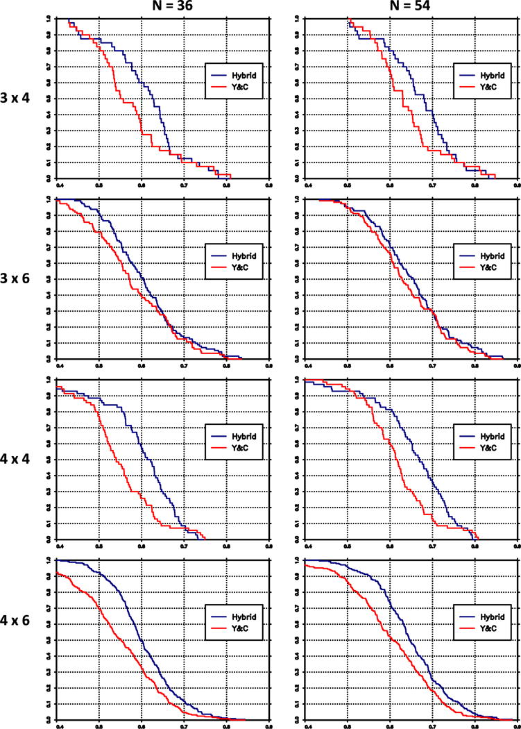
Survival distributions of accuracy index, averaged over groups, hybrid method (blue), and Yuan–Chappell (Y&C) method (red).

Figure 2.

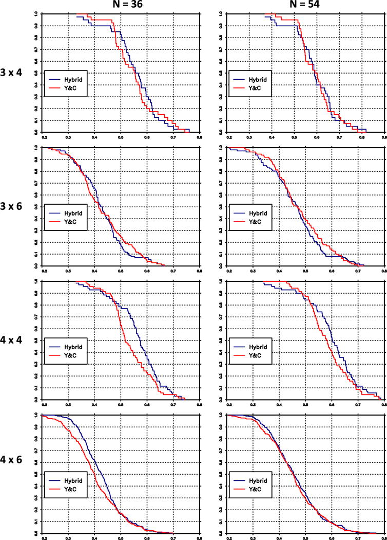
Survival distributions of percent correct selection (PCS), averaged over groups, hybrid method (blue), and Yuan–Chappell (Y&C) method (red).

5. Discussion

We have proposed a new method for more than two completely or partially ordered groups. In the case of completely ordered groups, for the scenarios we considered in this paper, the proposed method has properties that are at least as good as those for the method of Yuan and Chappell [22]. To our knowledge, no other method has been proposed for partially ordered groups.

There are several open areas of research under consideration. A reviewer suggested that an alternative to averaging the Hwang–Peddada estimates (2) over the initial guesses at the unknown orders is to choose the ordering that is ‘most plausible’. This could be performed by choosing the ordering with the greatest likelihood, or highest posterior probability, if priors are placed on the initial guesses at the unknown orders. The reviewer also suggested that the use of the same skeleton in each group, based on [27], might be replaced by a skeleton that reflected the complete or partial order. One could argue that the use of a common skeleton represents an initial skepticism about the magnitude of the group effect and that in general, the CRM is robust to the choice of the skeleton. These would imply that using different skeletons in the groups would not change the operating characteristics by much, but this is a question that have not been investigated.

Another open question concerns the choice of weights in (6). All of the simulations in this paper used equal weights, and we are currently investigating how much the operating characteristics change if these weights correctly reflected population proportions. If unequal weights are used, it is not known the effect of misspecifying the population proportions.

References

- 1.Ramanathan R, Egorin M, Takimoto C, Remick S, Doroshow J, LoRusso P, Mulkerin D, Grem J, Hamilton A, Murgo A, Potter D, Belani C, Hayes M, Peng B, Ivy P. Phase I and pharmacokinetic study of imatinib mesylate in patients with advanced malignancies and varying degrees of liver dysfunction: a study by the national cancer institute organ dysfunction working group. Journal of Clinical Oncology. 2008;26:563–569. doi: 10.1200/JCO.2007.11.0304. [DOI] [PubMed] [Google Scholar]
- 2.LoRusso P, Venkatakrishnan K, Ramanathan R, Sarantopoulos J, Mulkerin D, Shibata S, Hamilton A, Dowlati A, Mani S, Rudek M, Takimoto C, Neuwirth R, Esseltine D, Ivy P. Pharmacokinetics and safety of bortezomib in patients with advanced malignancies and varying degrees of liver dysfunction: phase I NCI Organ Dysfunction Working Group Study NCI-6432. Clinical Cancer Research. 2012;18(10):1–10. doi: 10.1158/1078-0432.CCR-11-2873. [DOI] [PMC free article] [PubMed] [Google Scholar]
- 3.Leal T, Remick S, Takimoto C, Ramanathan R, Davies A, Egorin M, Hamilton A, LoRusso P, Shibata S, Lenz H-J, Mier J, Sarantopoulos J, Mani S, Wright J, Ivy S, Neuwirth R, von Moltke L, Venkatakrishnan K, Mulkerin D. Dose-escalating and pharmacological study of bortezomib in adult cancer patients with impaired renal function: a National Cancer Institute Organ Dysfunction Working Group Study. Cancer Chemotherapy and Pharmacology. 2011;68:1439–1447. doi: 10.1007/s00280-011-1637-5. [DOI] [PMC free article] [PubMed] [Google Scholar]
- 4.Kim K-P, Kim H-S, Sym S, Bae K, Hong Y, Chang H-M, Lee J, Kang Y-K, Lee J, Shin J-G, Kim T. A UGT1A1*28 and *6 genotype-directed phase I dose-escalation trial of irinotecan with fixed-dose capecitabine in Korean patients with metastatic colorectal cancer. Cancer Chemotherapy and Pharmacology. 2013;71:1609–1617. doi: 10.1007/s00280-013-2161-6. [DOI] [PubMed] [Google Scholar]
- 5.Satoh T, Ura T, Yamada Y, Yamazaki K, Tsujinaka T, Munakata M, Nishina T, Okamura S, Esaki T, Sasaki Y, Koizuma W, Kakeji Y, Ishizuka N, Hyodo I, Sakata Y. Genotype-directed, dose-finding study of irinotecan in cancer patients with UGT1A1*28 and or UGT1A1*6 polymorphisms. Cancer Science. 2011;102:1868–1873. doi: 10.1111/j.1349-7006.2011.02030.x. [DOI] [PubMed] [Google Scholar]
- 6.Innocenti F, Schilsky R, Ramrez J, Janisch L, Undevia S, House L, Das S, Wu K, Turcich M, Marsh R, Karrison T, Maitland M, Salgia R, Ratain M. Dose-finding and pharmacokinetic study to optimize the dosing of irinotecan according to the UGT1A1 genotype of patients with cancer. Journal of Clinical Oncology. 2014;32(22):2328–2334. doi: 10.1200/JCO.2014.55.2307. [DOI] [PMC free article] [PubMed] [Google Scholar]
- 7.Conaway M, Dunbar S, Peddada S. Designs for single- or multiple-agent phase I trials. Biometrics. 2004;60:661–669. doi: 10.1111/j.0006-341X.2004.00215.x. [DOI] [PubMed] [Google Scholar]
- 8.Wages N, Conaway M, O’Quigley J. Continual reassessment method for partial ordering. Biometrics. 2011;67:1555–1563. doi: 10.1111/j.1541-0420.2011.01560.x. [DOI] [PMC free article] [PubMed] [Google Scholar]
- 9.Wages N, Conaway M, O’Quigley J. Dose-finding design for multi-drug combinations. Clinical Trials. 2011;8:380–389. doi: 10.1177/1740774511408748. [DOI] [PMC free article] [PubMed] [Google Scholar]
- 10.Wages N. Identifying a maximum tolerated contour in two-dimensional dose finding. Statistics in Medicine. 2017;36:242–253. doi: 10.1002/sim.6918. [DOI] [PMC free article] [PubMed] [Google Scholar]
- 11.Thall P, Millikan R, Mueller P, Lee S. Dose-finding with two agents in phase I oncology trials. Biometrics. 2003;59:487–496. doi: 10.1111/1541-0420.00058. [DOI] [PubMed] [Google Scholar]
- 12.O’Quigley J, Shen L, Gamst A. Two sample continual reassessment method. Journal of Biopharmaceutical Statistics. 1999;9:17–44. doi: 10.1081/BIP-100100998. [DOI] [PubMed] [Google Scholar]
- 13.Legezda A, Ibrahim J. Heterogeneity in phase I clinical trials: prior elicitation and computation using the continual reassessment method. Statistics in Medicine. 2001;20:867–882. doi: 10.1002/sim.701. [DOI] [PubMed] [Google Scholar]
- 14.O’Quigley J, Paoletti X. Continual reassessment method for ordered groups. Biometrics. 2003;59:430–440. doi: 10.1111/1541-0420.00050. [DOI] [PubMed] [Google Scholar]
- 15.Ivanova A, Wang K. Bivariate isotonic design for dose-finding with ordered groups. Statistics in Medicine. 2006;25:2018–2026. doi: 10.1002/sim.2312. [DOI] [PubMed] [Google Scholar]
- 16.Wages N, Read P, Petroni G. A Phase I/II adaptive design for heterogeneous groups with application to a stereotactic body radiation therapy trial. Pharmaceutical Statistics. 2015;14(4):302–310. doi: 10.1002/pst.1686. [DOI] [PMC free article] [PubMed] [Google Scholar]
- 17.O’Quigley J. Phase I and phase I/II dose finding algorithms using continual reassessment method. In: Crowley J, Ankherst D, editors. Handbook of Statistics in Clinical Oncology. 2nd. Chapman and Hall/CRC Biostatistics Series; Boca Raton, FL: 2006. [Google Scholar]
- 18.O’Quigley J, Iasonos A. Bridging solutions in dose-finding problems. Journal of Biopharmaceutical Statistics. 2014;6(2):185–197. doi: 10.1080/19466315.2014.906365. [DOI] [PMC free article] [PubMed] [Google Scholar]
- 19.O’Quigley J. Theoretical study of the continual reassessment method. Journal of Statistical Planning and Inference. 2006;136(6):1765–1780. [Google Scholar]
- 20.Conaway M, Wages N. Designs for phase I trials in ordered groups. Statistics in Medicine. 2017;36(2):254–265. doi: 10.1002/sim.7133. [DOI] [PMC free article] [PubMed] [Google Scholar]
- 21.Hwang J, Peddada S. Confidence interval estimation subject to order restrictions. The Annals of Statistics. 1994;22:67–93. [Google Scholar]
- 22.Yuan Z, Chappell R. Isotonic designs for phase I cancer clinical trials with multiple risk groups. Clinical Trials. 2004;1(6):499–508. doi: 10.1191/1740774504cn058oa. [DOI] [PubMed] [Google Scholar]
- 23.Robertson T, Wright FT, Dykstra R. Order Restricted Statistical Inference. J. Wiley New York; New York, NY: 1988. [Google Scholar]
- 24.Kelly R. Stochastic reduction of loss in estimating normal means by isotonic regression. The Annals of Statistics. 1989;17(2):937–940. [Google Scholar]
- 25.Lee C-I. Quadratic loss of order restricted estimators for treatment means with a control. The Annals of Statistics. 1988;16(2):751–758. [Google Scholar]
- 26.Wages N, Conaway M. Specifications of a continual reassessment method design for phase I trials of combined drugs. Pharmaceutical Statistics. 2013;12:217–224. doi: 10.1002/pst.1575. [DOI] [PMC free article] [PubMed] [Google Scholar]
- 27.Lee S, Cheung YK. Model calibration in the continual reassessment method. Clinical Trials. 2009;6:227–238. doi: 10.1177/1740774509105076. [DOI] [PMC free article] [PubMed] [Google Scholar]
- 28.Mander A, Sweeting M. A product of independent beta probabilities dose escalation (PIPE) design for dual-agent phase I trials. Statistics in Medicine. 2015;34(3):1261–1276. doi: 10.1002/sim.6434. [DOI] [PMC free article] [PubMed] [Google Scholar]
- 29.Whitehead J, Williamson D. Bayesian decision procedures based on logistic regression models for dose-finding studies. Journal of Biopharmaceutical Statistics. 1998;8:445–467. doi: 10.1080/10543409808835252. [DOI] [PubMed] [Google Scholar]
- 30.Cheung YK. Dose Finding by the Continual Reassessment Method. Chapman and Hall/CRC Biostatistics Series; Boca Raton, FL: 2011. [Google Scholar]
Associated Data
This section collects any data citations, data availability statements, or supplementary materials included in this article.