Tree-based identification of subgroups for time-varying covariate survival data

SUMMARY

Classification and regression tree (CART) analyses identify subsets of a sample that differ on an outcome. Discrimination of subsets is performed using recursive binary splitting on a set of covariates, allowing for interactions of variable subgroups not easily captured in standard model building techniques. Using CART with epidemiological data can be problematic as there is often a need to adjust for potential confounders and to account for time-varying covariates in the context of right-censored survival data. While CART variations exist individually for survival analysis, time-varying covariates and incorporating possible confounders, examples of CART using all three together are lacking. We propose a method to identify subsets of time-varying covariate risk factors that affect survival while adjusting for possible confounders. The technique is demonstrated on data from the Bypass Angioplasty Revascularization Investigation 2 Diabetes clinical trial to find combinations of modifiable time-varying cardiac risk factors (e.g. smoking status, blood pressure, lipid levels, and HbA1c level) that are associated with time-to-event clinical outcomes.

1. INTRODUCTION

Biological paradigms of disease progression involve multiple risk factors working in conjunction with one another. Yet, the analysis of epidemiological data often utilizes simplified statistical models to identify risk factors and to describe these complex biological systems. Common models for survival data include Cox proportional hazards regression models and survival classification and regression trees (CART). The Cox model estimates the effect of covariates on the multiplicative variation of the unknown and unspecified baseline hazard and can incorporate time-varying covariates and adjustments for potential confounders. Forward selection algorithms are frequently used to build Cox models; however, they do not easily accommodate the detection of complicated interactions among covariates. Alternatively, CART analyses identify complex interactions of covariate subgroups based on the prognosis for the outcome. Variations of CART have been developed for survival data, time-varying covariates and potential confounding variables separately, but not for all three combined.

This work is motivated by Bypass Angioplasty Revascularization Investigation 2 Diabetes (BARI 2D)¹, a randomized clinical trial including participants with both type 2 diabetes and coronary artery disease. Our goal was to analyze the effect of the non-randomized control status of seven modifiable cardiac risk factors (or combinations) on survival. The risk factors were measured repeatedly over the course of the trial, and we hypothesized that the effect of one factor on mortality depended on the level of other factors. As a result, in this paper we develop a tree-based survival model incorporating time-varying covariates and adjustments for potential confounding variables.

This paper is organized as follows. Section 2 introduces the BARI 2D trial. Section 3 reviews existing methodologies and applies them to BARI 2D. Section 4 proposes a method for tree-based modeling with adjusted time-varying survival data and applies it to BARI 2D. We conclude with a discussion.

2. BARI 2D TRIAL

The BARI 2D randomized trial was to determine the optimal 5-year treatment plan for participants with type 2 diabetes and documented coronary artery disease ^2–4. The trial had a 2×2 factorial design to simultaneously randomize participants to 1) a cardiac treatment strategy comparing prompt revascularization versus medical therapy with as-needed revascularization, and 2) a diabetes treatment strategy comparing primarily insulin sensitizing versus insulin providing drug therapy. The trial started January 2001 and completed follow-up of the 2,368 participants in November 2008. There were a total of 316 deaths with an overall survival of 88.0% at 5 years. The results showed no significant differences between either the cardiac strategies or the diabetes strategies on mortality¹.

All participants in the BARI 2D trial had intensive medical therapy to control modifiable cardiac risk factors, including low density lipoproteins (LDL), non-high density lipoproteins (non-HDL), triglycerides (TG), blood pressure (systolic and diastolic, SBP and DBP respectively), hemoglobin A1c (HbA1c) and smoking status. As a secondary non-randomized analysis, we aim to identify combinations of these risk factors that are associated with long-term survival. The risk factors, target goals, collection schedules and modeling notes are in Table 1. Ninety-five (95) percent of participant visits contained up-to-date risk factor information at that visit. Visits with partial risk factor data were not included the analysis. Participants who missed visits carried previous visit information forward up to 15 months.

Table 1.

Cardiac Risk Factors in BARI 2D

Risk Factor	Goal1	Collection Schedule	Parameterization
LDL	<100 mg/dL	Baseline, 6 months, 1 year and annually thereafter	Indicator variables model three groups; LDL<100, LDL>100 and LDL not computed as Triglycerides > 400
Non-HDL	<130 mg/dL		Indicator variable indicating in-control status
Triglycerides	<150 mg/dL		Indicator variable indicating in-control Status
Blood Pressure	SBP <130 mmHg DBP <80 mmHg	Baseline, monthly for the first 6 months, and quarterly thereafter	Indicator variables modeled 4 in- vs. out-of control groups due to high correlations
HbA1c	<7.0%	Baseline, 1 month, 3 months, 6 months and semi-annually thereafter	Indicator variable indicating in-control status
Smoking	Non-smoker	Baseline and annually thereafter	Indicator variable indicating in-control status

¹From the American College of Cardiology and/or the American Diabetes Association

Cardiac risk factor status in the BARI 2D trial changed as the trial progressed. Table 2 shows the proportion of three-year survivors meeting the goals at baseline and years 1, 3 and 5. The significant jump between baseline and one year in the percentage of participants meeting the risk factor goals reflects the initiation of intensive medical therapy. After year 1, there was a significant continual improvement in the percentage of three year survivors meeting each risk factor goal with the exception of smoking status (baseline to one year improvement was maintained) and HbA1c (initial improvement eroded).

Table 2.

Change in BARI 2D Risk Factor Control Status

Risk Factor	Percent of Participants In Control†				Jump* p-val	Slope* p-val
	Baseline	Year 1	Year 3	Year 5
LDL-C	60	75	83	85	<0.0001 Jump	<0.0001 Improve
Non-HDL-C	54	71	79	83	<0.0001 Jump	<0.0001 Improve
Triglycerides	51	57	61	64	0.005 Jump	<0.0001 Improve
Systolic BP	50	56	62	62	0.0013 Jump	<0.0001 Improve
Diastolic BP	69	71	75	79	0.64 No Jump	<0.0001 Improve
Non-Smoker	88	90	91	91	0.0013 Jump	0.12 Maintain
A1C	40	51	48	46	<0.0001 Jump	<0.0001 Degrade
Meet all goals	6	10	13	13	<0.0001 Jump	0.13 Maintain

^*p-values computed using a GEE logit(meet goal) = B0+B1*baseline +B2* year, taking into account multiple observations per participant. Baseline is an indicator variable for the baseline value and year is continuous year of follow-up (0–5). Testing the significance of B1 is testing if the baseline value can be predicted by the same slope as the year 1–5 data. The jump p-value corresponds to the test B1=0. The slope p-value corresponds to the test B2=0. Significance tests based on N=1854 participants with complete data at each of baseline, year 1 and year 3.

^†N=1854. These include three year survivors who had complete data at each of the baseline, year 1 and year 3 visits. At year 5, N=1062 due to late recruitment, loss to follow-up and deaths. Analysis restricted to reflect changes in risk factor status of individuals across time. Allowing all data to be used (not restricting to 3-year survivors with baseline, year 1 and year 3 visits) the percentages in the above table change less than 2% and the conclusion from the tests remain the same, with all significant p-values < 0.001 and all non-significant p-values > 0.075.

When modeling survival differences based upon risk factor status, potential confounding variables need to be identified. In BARI 2D, clinical experts determined the following confounding variables: baseline age, gender, race/ethnicity, randomization group, randomization strata, geographic region, and year of randomization.

3. REVIEW OF EXISTING METHODS AND THEIR APPLICATION

3.1 Cox Models

Cox proportional hazard models ⁵ and their many variations are commonly used in epidemiological literature to analyze time-to-event survival data. Descriptions can be found with varying degrees of statistical sophistication^6–9.

The methods in this paper include both time-varying and non time-varying covariates. The time-varying covariates are modeled with the counting process formulation of the Cox model^{6, 9} and require specification of the time interval(s) on which each participant has constant risk factor data. This formulation allows discontinuous intervals of risk so participants can come in and out of the analysis corresponding to the time periods when they have measured data. Non time-varying covariates specify that the participant has constant risk factor data over the entire study. In the CART analyses below, the Cox regression uses either constant (baseline or year 1) or time-varying risk factor data, while the potential confounders are constant. It is straightforward to allow the confounders to be time-varying, but not needed in our application.

An initial time-varying Cox model analyzed the 2,265 participants (46,733 or 95% of clinic visits) who had all seven risk factors up-to-date at any visit (103 participants did not have all seven risk factors for any visit). The effect of in-control (IC) cardiac risk factors, compared to not-in-control (NIC), on survival with time-varying risk factor status was estimated in SAS 9.3 with PROC PHREG. A forward stepwise selection algorithm, which forced the confounding variables into all models, was used to determine the set of significant risk factors. Table 3 contains the results, with non-HDL and smoking status risk factors retaining significance. A backward stepwise selection algorithm resulted in the same final model. The interaction between the significant main effects was not significant. Given the aim to identify complex combinations of subgroups of risk factors related to survival, the CART modeling techniques were next explored.

Table 3.

Results from time-varying risk factor Cox model for survival

Risk Factor	Hazard Ratio	p-value
Non-HDL in Control (reference = Non-HDL out of control)	0.61	0.0002
Non-Smoker (reference = current smoker)	0.63	0.0240
Non-HDL in control, Non-Smoker interaction	Not-significant and removed from the model

Adjusted for age of the participant at baseline, gender, race/ethnicity, randomization group, selected type of initial elective revascularization (surgical or catheter-based), geographic region, and year of randomization.

3.2 Survival CART models

CART techniques have been utilized in numerous epidemiological and public health fields^10–14 and are described elsewhere ^{15, 16}. CART analyses create subgroups based on complex combinations of covariate values that are related to an outcome (discrete or continuous). The popularity of CART began with the seminal work by Breiman et al. in 1984¹⁵. CART for survival data was introduced in 1985¹⁷, with subsequent modifications^{18, 19}. CART starts by splitting the participants into two subgroups (or nodes) that maximize the between node separation (for example, the largest difference between the two node survival curves). This continues recursively as each subsequent node is split into subgroups in the same fashion. CART has four distinct components¹⁹: 1) Questions, 2) Splits, 3) Size, and 4) Summary.

Questions

Determine the questions that will split participants. A CART analysis with survival data will split participants from a node by asking a yes/no question based on the outcome measure and the covariates of interest (for example, is there a difference in survival between participants whose baseline non-HDL is in-control versus baseline non-HDL is not-in-control?). Inclusion or exclusion from a given category (e.g. non-HDL in control) creates two participant subgroups representing a potential split.

Splits

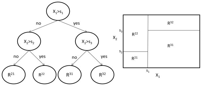
Define a goodness-of-split criterion to compare the potential splits. In survival CART, the two subgroups of each potential split have been compared using the non-parametric log-rank statistic ^{19, 20} and likelihood approaches ²⁰. Test statistics within Cox models have been used as a semi-parametric method that allows for the adjustment of covariates ¹³. A given node will likely have a number of potential splits (for example, splitting on the control status of non-HDL or TG or HbA1c). The potential split with the largest between node separations (for example, the largest χ² statistic in a Cox model) becomes the next split. Once a node is split into two leaves, the data from each leaf is split independently in a recursive fashion. This recursive binary partitioning has a one-to-one correspondence to a tree, see Figure 1.

Figure 1.

Recursive Binary Partition and Corresponding Tree

Size

Pre-specify when to stop growing a tree and the final tree construction. Examples include splitting nodes if there are any effect differences larger than a pre-specified threshold, any test statistics larger than a given number, splitting until a certain number of subgroups have been identified, or restrictions on the size of terminal nodes¹².

Summary

Provide statistical summaries for the final conclusion. Once a tree is compete, then summaries of that tree, or across many competing trees will be used to make conclusions. In public health literature, the terminal nodes of the tree are used in regression models for direct comparison of the groups^{10, 21, 22}.

BARI 2D Example

For the BARI 2D example, the split step takes into account the non-randomized comparison for the study by adjusting for potential confounding variables. Schmoor et al.¹³ used the Cox model with CART to adjust the treatment effect based upon prognostic subgroups. The example below uses an adjusted Cox model to determine which split creates the most disparate subgroups with respect to mortality.

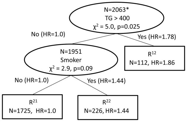
An initial survival tree adjusted for potential confounders was created to identify the baseline risk factor profiles relating to survival in BARI 2D. The baseline risk factor profiles reflect the participant’s health status prior to entering the trial. In the CART analysis, the questions were the control status of the various baseline risk factors; the split criteria was the baseline risk factor that had the largest χ² statistic in a Cox model including the confounding variables. The tree grew until there were no splits with a chi-square statistic of 2.0 or larger and then was pruned back to splits that had a chi-square statistic of 3.0 or larger. To summarize the tree, a final Cox model was run with the terminal node subgroups and the adjustment variables for direct comparison of all groups. The baseline risk factor tree is in Figure 2, where the intermediate nodes are represented with ovals and contain the number of participants in the node, the risk factor that will split that node and the test statistic and associated p-value of the comparison of the two branches of the node. The lines connecting the nodes contain the risk factor status of the previous node and the hazard ratios that were compared to determine the split. The terminal nodes are rectangles containing the number of people in the node and the hazard ratio from the resulting Cox model containing all of the terminal nodes and adjustment variables. Two baseline risk factors produced three terminal nodes based on TG and smoking status.

Figure 2.

Survival Tree based upon Baseline Risk Factor Status

*restricted to patients who have all 7 risk factors measured at baselines

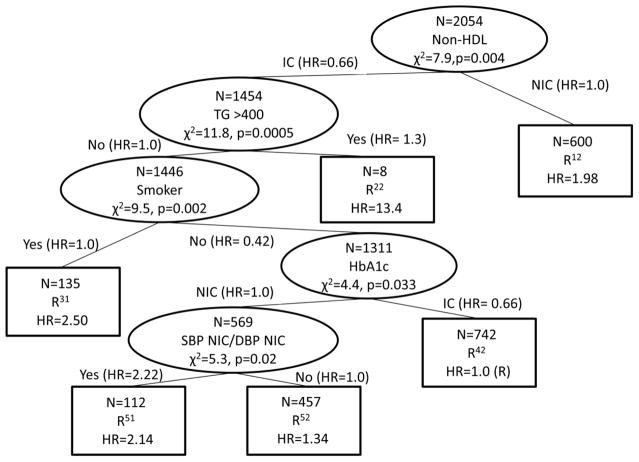
Similarly, an initial survival tree adjusted for potential confounders was created to identify the Year 1 risk factor profiles relating to survival in BARI 2D. The year 1 risk profile status reflects the participant’s health status after one year of intensive medical therapy. Table 2 demonstrated a jump between baseline and year 1 risk factor control for 6 of the 7 risk factors which may correspond to a different set of risk factors being associated with survival. In this CART analysis, the questions were the control status of the various year 1 risk factors, with splits, size and summary the same as the baseline risk factor table. In Figure 3, the tree based upon the year one risk factors contains six terminal nodes. The baseline tree (including TG and smoking status) can be seen embedded within the year 1 tree as the two nodes after the primary split of the non-HDL risk factor. The other risk factors identified in the tree to make subgroups included HbA1c, and the combination of NIC SBP and NIC DBP.

Figure 3.

Survival Tree based upon Year 1 Risk Factor Status

4 TIME-VARYING COX MODELS WITHIN CART

4.1 Tree-Based Algorithm for Survival Data with Time-Varying Covariates

The main obstacle to implementing time-varying covariates in the CART algorithm is splitting the data into nodes. The CART analysis defined thus far splits participants into the nodes. When incorporating time-varying covariates, the path the participant takes in the tree depends on the status of the risk factors at a given point in time. To develop the tree-based algorithm with time-varying covariates, we use a time varying Cox model and split participant visits.

Questions (Time-Vary)

The questions still regard survival experience given various risk factor control status, but now it allows the risk factor control status to be time-varying (previous examples used baseline or year 1 risk factor status).

Splits (Time-Vary)

Split the participant visits into nodes; the counting process derivation of the time-varying Cox model allows discontinuous time intervals. This allows a participant to be in one node during some time intervals and in another node during different time intervals. The risk factor with the largest test statistic within the adjusted time-varying Cox model is the next split.

The time-varying Cox model can be used with CART in two different ways. Similar to existing CART methods, the time-varying Cox model can be run recursively within each node separately using only the data from the participants while they are in that node. The second way is to use a forward stepwise splitting procedure which incorporates all of the data when determining the next split. These two methods are explored next using the BARI 2D Example.

BARI 2D Example - Recursive Splitting

The first node of the tree is determined by identifying the risk factor (RF_i, i=1, …, p) that maximizes the chi-square statistic corresponding to the test of H₀: β_RFi=0 vs. H_a: β_RFi ≠ 0 in the Cox model

$$\lambda [t\mid x,z]={\lambda }_0(t)\text{exp}(Z_{\mathit{RFi}}{(t)}^{\prime }{\beta }_{\mathit{RFi}}+X^{\prime }\beta )$$ (1)

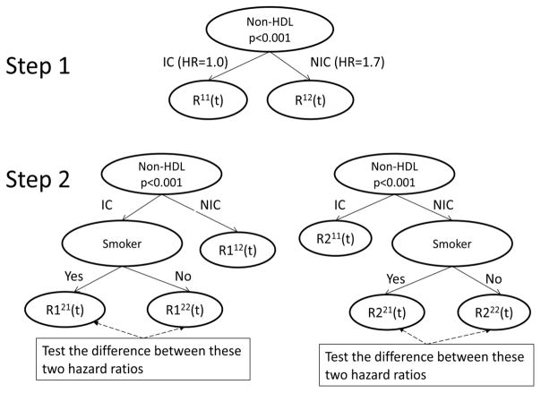
where Z_RFi(t) are indicator variables for individual risk factors as described in Table 1 and the X variables are the confounding variables. Suppose that non-HDL control status has the largest chi-square statistic and is the first node in the tree (see Figure 4, step 1). Two leaves are created corresponding to the IC (R¹¹(t)) and NIC (R¹²(t)) non-HDL status.

Figure 4.

First Split and Candidate Trees for the Second Split in the BARI 2D Data

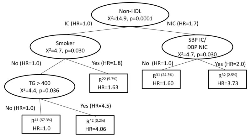
To determine the second split, compare all the potential splits to determine which has the highest χ² statistic. Using only the visits in the R¹¹(t) node, use an adjusted Cox model to obtain the χ² statistics corresponding to a split of the R¹¹(t) node. One potential split corresponds to the smoking status, which would create the tree on the left panel of Step 2 in Figure 4. An analogous potential split using only the nodes from R¹²(t) is shown in the right panel of Step 2 in Figure 4. All potential next splits are then compared and the split with the maximum chi-square statistic becomes the next split. This is continued recursively until no more splits meet the size criteria. The final tree is in Figure 5. In addition to non-HDL and smoking status, the final tree also includes SBP IC and DBP NIC, along with TG >= 400.

Figure 5.

Adjusted Time-Varying Survival CART: Recursive Splitting for BARI 2D Risk Factor Data

This method has the advantage of following the CART methodology in keeping the split decision as a local criteria, using only the data from the node to determine its split, allowing for time-varying covariates within CART and adjusting for potential confounding variables. A potential disadvantage is that it allows for different effects of the confounding variables at each step. Trees in epidemiological literature are often summarized by including the final prognostic subgroups in one adjusted Cox model for direct comparison of subgroup hazard ratios. Allowing different effects of confounding variables at each step of the creation of the tree may create subgroups that are not as disparate when the effects of the confounding variables are forced to be common in the final summary.

BARI 2D Example - Forward Stepwise Splitting

An alternative to the recursive splitting of the participant visit data is to utilize a forward stepwise splitting method. This method retains all prognostic subgroups in the model when determining the next split and is a restricted forward stepwise model selection.

The first node of the tree is determined similar to the recursive splitting algorithm, by identifying the risk factor (RF_i, i=1, …, p) that maximizes the χ² statistic corresponding to the test H₀: β_RFi=0 vs. H_a: β_RFi ≠ 0 in the Cox model in Equation 1.

To determine the second split, create subgroups that represent splits on the tree and use an adjusted Cox model to obtain the χ² statistics corresponding to each potential split. For example, below is the model to determine the χ² statistic on the left panel of step 2 in Figure 4 which includes indicator variables for each potential subgroup along with the adjustment variables:

$$\lambda [t\mid x,z]={\lambda }_0(t)\text{exp}(I_{R121}{(t)}^{\prime }{\beta }_{R121}+I_{R122}{(t)}^{\prime }{\beta }_{R122}+I_{R112}{(t)}^{\prime }{\beta }_{R112}+X^{\prime }\beta )$$

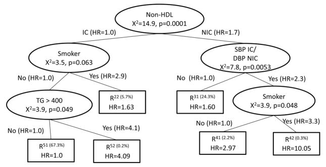
The χ² statistic associated with the test H₀: β_R121=β_R122 vs. H_a: β_R121≠ β_R122 would be compared across all potential risk factor splits. A potential split of the R1¹²(t) node is shown in the right panel of Step 2 in Figure 4. All potential next splits are then compared and the split with the maximum χ² statistic testing the equality of the hazard ratio of the two newly created nodes becomes the next split. This is continued until no more splits meet the size criteria. The final tree is in Figure 6. Note that the final result is very similar to the recursive splitting method in Figure 5, with one additional split of smoking status.

Figure 6.

Adjusted Time-Varying Survival CART: Forward Stepwise Splitting for BARI 2D Risk Factor Data

This method has the advantage of allowing for time-varying covariates within CART, adjusting for potential confounding variables and consistency between the tree building and the summary with regards to the confounding variable effects. A disadvantage is that it is more complicated to program into software packages.

4.2 Model Validation

Training and testing sets are often used in non-survival CART analyses to compute misclassification rates or mean squared errors for validation of the model. In the non-adjusted non-time-varying survival setting²³, the survival curve for each terminal node can be estimated based on the model from the training set. Then a Kaplan –Meier curve can be used to estimate the survival curves of the terminal nodes using the testing set. The predicted versus observed survival curves can be tested with a log-rank statistic. It is not clear how to extend this type of validation to survival CART with adjustment and time-varying covariates.

Instead of training and testing sets, we validated the model by estimating a time-varying Cox model that forced the main effects and pair wise interactions of all the risk factors. Pair wise interactions with a p-value of > 0.05 were removed using a backward stepwise algorithm. All non-significant risk factor main effects were removed so long as they were not in any interaction terms. This model retained Non-HDL IC, Smoking IC, (SPB IC and DBP NIC) and an interaction between Non-HDL IC and (SBP IC and DBP NIC). Note this is a very similar model to Figures 6 and 7. Figure 6 contains smoking status on both sides of the original Non-HDL split, indicting possible main effect status in the model. In the CART analysis, SBP IC/DBP NIC was the strongest risk factor in the non-HDL NIC branch, and was not present in the Non-HDL IC branch, indicating an interaction. This model had an AIC of 4020.8 and a BIC of 3948.5.

For the CART model in Figure 6, the AIC is 4023.4 and the BIC is 3947.5, slightly worse than the backward stepwise model using 0.10 as p-to-enter and p-to-stay using AIC, but slightly better from the same model using BIC.

4.3 Variations of this model

As with any tree-based method, there are many variations to be decided upon on a case-by-case basis. In split steps above, the subgroups were divided based upon the size of the test statistics or p-value comparing the equality of hazards in the newly created groups. This is a local decision as it is determined primarily by the data in the subgroup being split and follows the spirit of CART analyses to identify disparate groups. An alternate local criterion could be to predefine a minimally significant difference between the groups.

Alternatively, a more global model fitting criteria could be used such as BIC. If the group being split does not contain many participant visits, the resulting subgroups may have significantly different hazards but may not improve the model enough to improve the overall BIC. Other global criteria have involved penalties for misclassification and these can be incorporated into the proposed algorithm.

The CART literature is full of methods on final tree construction, including growing and pruning¹⁵, bagging²⁴, boosting^25–27, cross validation²⁸, random forests¹² and others. These concepts could be used with the method proposed in this paper; however the programming complexities of each method have not been explored here.

There is no reason to restrict the analysis specifically to the Cox model. The forward stepwise splitting method can be used with any model, including generalized linear models or generalized estimating equations.

5. DISCUSSION

The proposed algorithm incorporates the complex subgroups of a CART analysis and the flexibility of a time-varying Cox analysis for the evaluation of time-varying survival data. As such, the algorithm has all the strengths and weaknesses of both CART and greedy step-wise modeling techniques. The strengths include finding complex subsets of the data that affect the outcome, an intuitive way to add the variables by order of significance and clinicians are familiar with the concept of greedy algorithms. Weaknesses of CART methods are summarized elsewhere¹⁶ and include the handling of missing values, instability of trees due to overfitting, lack of smoothness and difficulty in capturing additive structures. Literature on the weaknesses of greedy algorithms is vast and a sample is included in the references^29–33, including overstating the significance of the results and not optimizing a reasonable criterion function. The method proposed here should be used as an exploratory tool as the results are specific to the dataset and need external validation with independent data before they can inform policy.

In the BARI 2D example, there are a number of interesting findings. The standard time-varying Cox analysis in section 3.1 indicated that non-HDL and smoking were the two significant risk factors. The adjusted survival CART based on baseline risk factor status in section 3.4 indicated that triglycerides and smoking status were significant factors. The adjusted survival CART based upon the year one risk factor status was comparatively large. There are a number of potential reasons for the baseline and year 1 differences. The larger tree at year 1 could reflect the participant’s biological transitions from the improvements in risk factor control status from entering the clinical trial. The lag time between risk factor control and clinical prognosis is not known. The size of the tree could also represent the heterogeneity of timing for an individual to reach in-control status, for example one participant could have reached control on day 2 while another could have reached control on day 364. It is also possible that the year 1 risk factor tree is over-fitting the data and finding too many significant splits. The standard CART methods to combat over-fitting could be applied to investigate this.

The final time-varying trees (both the recursive and forward stepwise splitting) have similarities to all of the preliminary analyses, especially with the inclusion of smoking status and triglycerides >=400. Non-HDL status was not included in the baseline risk factor tree, but was the primary split in both the year 1 and time-varying tree. The one year risk factor tree and the time-varying tree both contain a blood pressure risk factor, with the one year risk factor tree contain both SBP NIC and DBP NIC and the time varying tree indicating a low pulse pressure with SPB IC and DBP NIC. Finally, the year 1 tree is the only one that includes HbA1c as a risk factor.

There are many interesting extensions to this research that are conceptually possible, but computationally challenging. For example, with the BARI 2D data, there may be a possible lag time between the changes in risk factor status and the resulting effect on the outcome. This timing may differ for each risk factor and for each participant. A time lag could be incorporated into the Cox model to investigate the length of the lag and the homogeneity of lag times across risk factors. The analysis was described for categorical risk factor covariates. This can be extended to continuous risk factor covariates, though the computing is expected to be tedious. Finally, an interesting extension would be to include random effects in the Cox model to investigate heterogeneity across people with common risk factor profiles and confounding variables.

References

- 1.Study Group BD. A Randomized Trial of Therapies for Type 2 Diabetes and Coronary Artery Disease. [accessed Jun 11];New England Journal of Medicine. 2009 360:2503–15. doi: 10.1056/NEJMoa0805796. [DOI] [PMC free article] [PubMed] [Google Scholar]
- 2.Barsness GW, Gersh BJ, Brooks MM, Frye RL. Rationale for the revascularization arm of the Bypass Angioplasty Revascularization Investigation 2 Diabetes (BARI 2D) Trial. Am J Cardiol. 2006;97:31G–40G. doi: 10.1016/j.amjcard.2006.03.011. [DOI] [PubMed] [Google Scholar]
- 3.Brooks MM, Frye RL, Genuth S, et al. Hypotheses, design, and methods for the Bypass Angioplasty Revascularization Investigation 2 Diabetes (BARI 2D) Trial. Am J Cardiol. 2006;97:9G–19G. doi: 10.1016/j.amjcard.2006.02.023. [DOI] [PubMed] [Google Scholar]
- 4.Magee MF, Isley WL. Rationale, design, and methods for glycemic control in the Bypass Angioplasty Revascularization Investigation 2 Diabetes (BARI 2D) Trial. Am J Cardiol. 2006;97:20G–30G. doi: 10.1016/j.amjcard.2006.02.024. [DOI] [PubMed] [Google Scholar]
- 5.Cox DR. Regression Models and Life-Tables. Journal of the Royal Statistical Society Series B-Statistical Methodology. 1972;34:187. [Google Scholar]
- 6.Kalbfleisch JD, Prentice RL. The statistical analysis of failure time data. 2. Hoboken, N.J: J. Wiley; 2002. p. xiii.p. 439. [Google Scholar]
- 7.Hosmer DW, Lemeshow S. Applied survival analysis : regression modeling of time to event data. New York: Wiley; 1999. [Google Scholar]
- 8.Vittinghoff E. Regression methods in biostatistics : linear, logistic, survival, and repeated measures models. New York: Springer; 2005. [Google Scholar]
- 9.Therneau TM, Grambsch PM. Modeling survival data : extending the Cox model. New York: Springer; 2000. p. xiii.p. 350. [Google Scholar]
- 10.Lemon SC, Roy J, Clark MA, Friedmann PD, Rakowski W. Classification and regression tree analysis in public health: Methodological review and comparison with logistic regression. Annals of Behavioral Medicine. 2003;26:172–81. doi: 10.1207/S15324796ABM2603_02. [DOI] [PubMed] [Google Scholar]
- 11.Kurt I, Ture M, Kurum AT. Comparing performances of logistic regression, classification and regression tree, and neural networks for predicting coronary artery disease. Expert Syst Appl. 2008;34:366–74. [Google Scholar]
- 12.Strobl C, Malley J, Tutz G. An introduction to recursive partitioning: rationale, application, and characteristics of classification and regression trees, bagging, and random forests. Psychol Methods. 2009;14:323–48. doi: 10.1037/a0016973. [DOI] [PMC free article] [PubMed] [Google Scholar]
- 13.Schmoor C, Ulm K, Schumacher M. Comparison of the Cox model and the regression tree procedure in analyzing a randomized clinical-trial. Statistics in Medicine. 1993;12:2351–66. doi: 10.1002/sim.4780122411. [DOI] [PubMed] [Google Scholar]
- 14.Bacchetti P, Segal MR. Survival trees with time-dependent covariates: Application to estimating changes in the incubation period of AIDS. Lifetime Data Analysis. 1995;1:35–47. doi: 10.1007/BF00985256. [DOI] [PubMed] [Google Scholar]
- 15.Breiman L, Friedman J, Olshen R, Stone C. Classification and Regression Trees. Pacific Grove: Wadsworth; 1984. [Google Scholar]
- 16.Hastie T, Tibshirani R, Friedman JH. The elements of statistical learning : data mining, inference, and prediction. 2. New York, NY: Springer; 2009. p. xxii.p. 745. [Google Scholar]
- 17.Gordon L, Olshen RA. Tree-Structured Survival Analysis. Cancer Treatment Reports. 1985;69:1065–9. [PubMed] [Google Scholar]
- 18.Leblanc M, Crowley J. RELATIVE RISK TREES FOR CENSORED SURVIVAL-DATA. Biometrics. 1992;48:411–25. [PubMed] [Google Scholar]
- 19.Segal MR. Regression Trees for Censored-Data. Biometrics. 1988;44:35–47. [Google Scholar]
- 20.Leblanc M, Crowley J. SURVIVAL TREES BY GOODNESS OF SPLIT. Journal of the American Statistical Association. 1993;88:457–67. [Google Scholar]
- 21.Fonarow GC, Adams KF, Abraham WT, Yancy CW, Boscardin WJ Grp ASACS. Risk stratification for in-hospital mortality in acutely decompensated heart failure - Classification and regression tree analysis. Jama-J Am Med Assoc. 2005;293:572–80. doi: 10.1001/jama.293.5.572. [DOI] [PubMed] [Google Scholar]
- 22.Lamborn KR, Chang SM, Prados MD. Prognostic factors for survival of patients with glioblastoma: Recursive partitioning analysis. Neuro-Oncology. 2004;6:227–35. doi: 10.1215/S1152851703000620. [DOI] [PMC free article] [PubMed] [Google Scholar]
- 23.Intrator O, Kooperberg C. Trees and splines in survival analysis. Statistical methods in medical research. 1995;4:237–61. doi: 10.1177/096228029500400305. [DOI] [PubMed] [Google Scholar]
- 24.Breiman L. Bagging predictors. Machine Learning. 1996;24:123–40. [Google Scholar]
- 25.Freund Y. Boosting a Weak Learning Algorithm by Majority. Information and Computation. 1995;121:256–85. [Google Scholar]
- 26.Freund Y, Schapire RE. A decision-theoretic generalization of on-line learning and an application to boosting. Journal of Computer and System Sciences. 1997;55:119–39. [Google Scholar]
- 27.Schapire RE. The Strength of Weak Learnability. Machine Learning. 1990;5:197–227. [Google Scholar]
- 28.Breiman L, Spector P. Submodel Selection and Evaluation in Regression - the X-Random Case. International Statistical Review. 1992;60:291–319. [Google Scholar]
- 29.Steyerberg EW, Eijkemans MJ, Habbema JD. Stepwise selection in small data sets: a simulation study of bias in logistic regression analysis. [accessed Oct];J Clin Epidemiol. 1999 52:935–42. doi: 10.1016/s0895-4356(99)00103-1. [DOI] [PubMed] [Google Scholar]
- 30.Harrell FE, Jr, Lee KL, Mark DB. Multivariable prognostic models: issues in developing models, evaluating assumptions and adequacy, and measuring and reducing errors. Stat Med. 1996;15:361–87. doi: 10.1002/(SICI)1097-0258(19960229)15:4<361::AID-SIM168>3.0.CO;2-4. [DOI] [PubMed] [Google Scholar]
- 31.Freedman DA. A Note on Screening Regression Equations. The American Statistician. 1983;37:152–5. [Google Scholar]
- 32.Chatfield C. Model Uncertainty, Data Mining and Statistical Inference. Journal of the Royal Statistical Society Series A (Statistics in Society) 1995;158:419–66. [Google Scholar]
- 33.Weisberg S. Applied linear regression. 3. Hoboken, N.J: Wiley-Interscience; 2005. p. xvi.p. 310. [Google Scholar]