

Summary
We propose a method for analyzing data which consist of curves on multiple individuals, i.e., longitudinal or functional data. We use a Bayesian model where curves are expressed as linear combinations of B-splines with random coefficients. The curves are estimated as posterior means obtained via Markov chain Monte Carlo (MCMC) methods, which automatically select the local level of smoothing. The method is applicable to situations where curves are sampled sparsely and/or at irregular time points. We construct posterior credible intervals for the mean curve and for the individual curves. This methodology provides unified, efficient, and flexible means for smoothing functional data.
Keywords: Bayesian nonparametric smoothing, B-splines, Functional data, Longitudinal data, Mixed models, MCMC
1. Introduction
In recent years, nonparametric analysis of longitudinal data has received an increasing amount of attention. This acceleration gained impetus after the publication of Ramsay and Silverman (1997), which popularized the term “functional data analysis” (FDA; coined in Ramsay and Dalzell, 1991) to describe nonparametric analyses of longitudinal data which focus on the curves themselves as the basic unit of data. Goals for a given FDA may include, for example, describing the major modes of functional variation in the data, exploring the individual variation of curves from overall mean trajectories, and characterizing the dependence of curves on covariates. For these purposes, methods such as functional principal components analysis (FPCA) and functional linear models, among others, have also been developed and applied (Ramsay and Silverman, 1997, 2002; Rice, 2004; Müller, 2005).
An important first step with many FDA techniques is smoothing the data to obtain individual curves for each subject. Initially, FDA encompassed mostly data which were frequently and regularly sampled across individuals (e.g., Rao, 1958; Besse and Ramsay, 1986; Rice and Silverman, 1991). However, FDA has been increasingly applied to data which may be sampled at time points differing in both number and timing across individuals. Moreover, some individual curves may be sampled at only a few time points. Such data are called “sparse” functional data. This article focuses primarily on developing a Bayesian nonparametric method appropriate for smoothing noisy, sparse functional data. This method can also be used, however, for smoothing functional data which are not sparse.
Many methods have been proposed for smoothing functional data. One approach, sometimes called the “direct method”, smooths each curve individually. This often works well when there are an equal number of frequently sampled time points for each individual under study. However, problems arise when attempting this direct method on sparse functional data. For example, individuals with few sampled time points will have unreliable curve estimates, especially if the data are noisy. Moreover, subsequent analyses utilizing the smoothed curves often give equal weight to curves which may in fact be estimated with varying levels of precision. In this situation, it would be desirable to borrow strength across individuals when estimating individual curves and also to adjust the levels of certainty to reflect both the variation within an individual and the variation across individuals in the sample.
One of the first methods aimed at smoothing irregularly sampled curves was formulated by Brumback and Rice (1998); these authors proposed a penalized smoothing spline mixed model, which was a generalization of the work of Kimmeldorf and Wahba (1970) to multiple curve estimation. Closely related approaches include varying coefficient models (Hoover et al., 1998), mixed effects smoothing splines (Wang, 1998), the functional mixed effects models of Guo (2002), and various methods employing B-splines for modeling functional data (Shi, Weiss, and Taylor, 1996; Rice and Wu, 2000; James, Hastie, and Sugar, 2001; James and Sugar, 2003). A recently developed adaptive smoothing methodology employing piecewise linear models and knot selection through reversible-jump MCMC (Holmes and Mallick, 2001) is given in Bigelow and Dunson (2005a,b).
Many of the approaches listed above require a separate model selection procedure distinct from parameter estimation to choose the level of smoothing in the model. Inference following parameter estimation often also requires an additional procedure (e.g., bootstrapping), and is conditional on the “best” model selected. This can lead to unrealistically low estimates of the level of variability in curve estimates. One remedy to these difficulties which is appropriate for sparse functional data and which elegantly handles many of the issues mentioned above is to use a Bayesian mixed effects model with a B-spline basis, employing an unknown number and locations of breakpoints. We use Markov chain Monte Carlo (MCMC) methods to sample from the posterior distribution of the model parameters. The model includes latent indicators which determine whether a given breakpoint is included in the model. Our strategy is to start with a large number of breakpoints and hence a large number of B-spline basis functions and then allow that each of these breakpoints may be excluded from the model with a nonzero probability. This method builds on previous work on nonparametric estimation of a single function (Smith and Kohn 1996; Kohn, Smith, and Chan, 2001). Our model also allows for straightforward computation of pointwise Bayesian posterior credible regions for both the mean curve and the individual curves. The individual posterior credible regions automatically adjust for the level of sparseness with which the given curve is sampled.
The outline for the remainder of the article is as follows. In Section 2, we describe the application data set obtained from the Massachusetts Institute of Technology (MIT) Growth and Development Study. In Section 3, we describe the proposed model, while Section 4 outlines the sampling scheme for this model. In Section 5, we analyze the data from the MIT Growth and Development Study. Section 6 provides the results of a simulation study. Finally, in Section 7, we present a short discussion and suggest areas of further development.
2. MIT Growth and Development Study
To demonstrate the proposed method, we apply it to the MIT Growth and Development Study (Bandini et al., 2002; Phillips et al., 2003) taken from Fitzmaurice, Laird, and Ware (2004). The data consist of body fat measurements on a cohort of 162 girls. The goal of the analyses in Fitzmaurice et al. (2004) is to examine the changes in body fat percentage before and after menarche. All of the girls were followed roughly annually from up to 6 years prior to menarche until 4 years afterward. An average of 6.4 measurements exist per individual but the actual number of measurements for each girl varies from 3 to 10. A plot of the body fat percentage measurements versus time can be observed in Figure 1. In this plot, time (in years) is centered at the onset of menarche, which corresponds to an average actual age of 12.8 years. In Fitzmaurice et al. (2004), a LOWESS curve is fit to the data to determine plausible models for the mean response. The LOWESS curve reveals an increase in the rate of body fat accretion after menarche; these authors subsequently fit a piecewise linear mixed-effects regression model with a single breakpoint at the onset of menarche.
Figure 1.
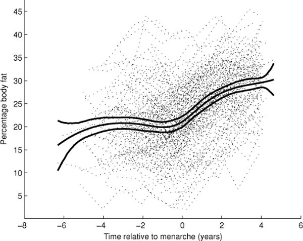
MIT Growth and Development Study: body fat percentages for 162 girls (dotted lines) and mean trajectory of body fat percentages with 95% posterior credible intervals (solid lines).
This piecewise linear model effectively captures the change-point in overall mean slope of body fat accretion pre- and postmenarche. However, the data also provide evidence suggesting that the rate of accretion somewhat slows again after 1 year postmenarche. This potentially more complex functional form for the overall mean is not captured by the piecewise linear model of Fitzmaurice et al. (2004). Moreover, some individual girls have trajectories which exhibit strong variation from the overall mean. One of the goals in an analysis of these data may be to estimate individual trajectories or to identify those trajectories which exhibit significantly unusual behavior. The piecewise linear model of Fitzmaurice et al. (2004) does not allow for sizeable variation in the shapes of the individual trajectories and hence is not well adapted to these types of analyses. For these reasons, it may be advantageous to examine the changes in body fat percentage before and after menarche via a more flexible smoothing methodology. In Section 5, we flexibly estimate and provide posterior credible intervals for the overall mean and individual girl body fat trajectories. Furthermore, we explore the major modes of functional variation and correlate these with age of onset of menarche by employing an eigenanalysis (FPCA) on the estimated covariance function of the random effects.
3. The Model and Prior Specification
3.1 The Model
Suppose we observe n individuals. The response yi(t) for individual i as a function of time t is assumed to be independent of responses from other individuals and to arise from the model
| (1) |
Here, μ(·) is the mean function for all individuals under study and gi(·) is the systematic departure of subject i from μ(t). We assume that the error function εi(·) is a zero mean Gaussian white-noise process with constant variance and is uncorrelated with μ(t) or gi(t). Other authors have considered models with serial correlation on the error terms. For simplicity, we do not consider such a case here.
We further suppose that model (1) can be closely approximated by expressing μ(·) and gi(·) as linear combinations of basis functions. We develop the case where the basis functions are chosen as B-splines of order p. In general, however, this method is easily generalizable to other types of basis functions, e.g., radial bases for bivariate surface estimation (Kohn et al., 2001). Let {B1(·), …, BK ()} be a given K-dimensional B-spline basis of order p spanning the range of time values [0, T]. Thus, we express model (1) as
| (2) |
Here, the coefficients βk correspond to the mean functional outcomes for all individuals under study, whereas the random coefficients bi = (bi1, …, biK)′ correspond to the “large-scale” deviation of the ith individual’s functional outcome from the mean. In Section 3.2, these random coefficients are modeled as independent random variables with covariance Σb. Along with the white-noise process εi(·), the covariance matrix Σb of the random effects determines the covariance structure of the within-individual functional observations.
Of course, only a finite number of observations, say mi, are made on each individual; the number and times of occurrence of these observations may vary considerably from one subject to another. Suppose that the ith individual has measurements at time points . Using (2), the observed outcomes yij are modeled as
| (3) |
Let Xi be the design matrix of dimensions mi × K for the ith subject with the jkth entry given by Bk(tij). Then (3) can be expressed in matrix form as
| (4) |
This is a random effects model with a within-subject covariance structure given by cov . Thus, if we condition the model on the choice of basis functions and treat the design matrix as fixed, parameter estimation can proceed using standard techniques, either Bayesian or non-Bayesian.
In practice, however, the number and placement of breakpoints determining the B-spline basis are seldom known a priori. One way to handle this in a Bayesian framework is to start with a large pool of potential breakpoints and include latent indicator variables in the model, with one for each breakpoint (Smith and Kohn, 1996; Kohn et al., 2001). A given indicator equals one if the corresponding breakpoint is to be included in the model and zero otherwise. Note that inclusion or exclusion of a breakpoint not only adds or deletes one basis function but also modifies those B-spline functions immediately surrounding it. Thus, the addition or deletion of breakpoints does not simply correspond to the addition or deletion of basis functions in model (4).
Let γ be the vector of indicator variables, and let be the qγ B-spline basis functions determined by the breakpoints selected in γ. Also, let Xγ,i denote the mi × qγ design matrix for subject i corresponding to these selected basis functions evaluated at time points ti. Then, model (4) conditional on γ becomes
| (5) |
The parameters βγ and are qγ-dimensional vectors corresponding to the model implied by the indicators γ. The relationship between the regression parameters conditional on γ and the regression parameters in the full model (4) is detailed in the Web Appendix. Note that we have formulated model (5) so that all subjects have the same basis functions. This implies that all individual trajectories can be well approximated by curves with the same level of smoothness. We indicate one way of relaxing this assumption in Section 7, where we also discuss the possible inclusion of covariates in model (5).
3.2 Prior Specification
We use a B-spline basis of order p over the range [0, T], where T is at least as large as the largest time point in the data. In our simulations and example, we use p = 4, thus generating piecewise cubic functions which are twice continuously differentiable at each breakpoint. One breakpoint is placed at each endpoint and at L interior points. The interior breakpoints can be placed on a fine regular grid or at prespecified quantiles of sampled time points. With L interior breakpoints, there are K = L + p basis functions of order p. Let γ = (γ1, …, γL)′ be the vector of latent indicator variables γl for inclusion of the lth interior breakpoint. The breakpoints at the endpoints are included with probability one. Thus, the model dimension conditional on γ is qγ = γ′γ + p.
Let be the regression and variance parameters of model (5) conditional on γ, with . For convenience when deriving the sampling scheme given in Section 4, we assume that the prior mean of the random effects bγ,i is βγ and re-express model (5) as
The prior specification is hierarchical with the priors on the parameters ζγ conditional on the indicators γ. The random effects bγ,i, i = 1, …, n are assumed a priori independent of multivariate normal distributions
where βγ is a qγ × 1 vector and Σb,γ is a qγ × qγ covariance matrix. The prior distribution of βγ is multivariate normal
| (6) |
where 0γ is a qγ vector of zeros and Iγ is the qγ × qγ identity matrix. The multiplier c is a prespecified constant; large values of c correspond to a vague prior for βγ.
We assume a priori that Σb,γ conditional on γ follows the “default conjugate prior” proposed by Kass and Natarajan (2006). In particular, this prior is the inverse Wishart, IW(ηb, ηbSγ), whose density is given by
To achieve vagueness, the degrees of freedom parameter is taken to be small (ηb = qγ), and the scale matrix Sγ is a minimally informative prior guess of Σb,γ. More specifically, Kass and Natarajan (2006) argue that represents vague knowledge on Σb,γ but because this choice varies with i, they suggest replacing it with its harmonic mean over the subjects, resulting in . We modify this slightly by replacing with a precalculated, data-dependent (e.g., REML) estimate . This is done to preserve the simplicity of the Gibbs sampling implementation of the MCMC algorithm in Section 4. Although this prior is data dependent, Kass and Natarajan (2006) note that it has asymptotically negligible effect on the posterior. The prior on is inverse gamma (IG)
where cε and dε are specified constants; values close to zero result in relatively vague priors.
Finally, we place a prior distribution on γ. The indicators γl, l = 1, …, L, are assumed a priori independent Bernoulli with parameter π, that is,
The hyperprior on π is beta(cπ, dπ), where cπ and dπ can be chosen to give a specified a priori expectation and standard deviation of the number of breakpoints included in the model (see Kohn et al., 2001). In our experience, the choice of cπ and dπ has minimal effect on the breakpoint selection when implementing the sampling scheme outlined in the next section.
4. Bayesian Inference
4.1 The Sampling Scheme
In this section, we outline the sampling scheme for our proposed model. More details on the sampling scheme and the posterior conditional distributions of the parameters are provided in the Web Appendix. Suppose that are the current draws for the parameters of model (5). Note that π has been integrated out, so that drawing π is unnecessary. The sampling scheme in the following iteration is as follows:
Step 1: Sample s distinct values l = {l1, …, ls} (for predetermined 1 ≤ s ≤ L) from {1, …, L} without replacement such that each such vector is equally probable. This step determines which latent indicator variables will be drawn in Step 2.
- Step 2: Sample from , where is the vector of indicators in γ0 not indexed by l. The parameters are sampled simultaneously to obtain a more efficient algorithm, because these parameters tend to be highly correlated with each other. Step 2 is carried out in three substeps:
- Step 2(a): Sample from , where u ranges over all s-dimensional vectors of zeros and ones, and Lu and Θu are given by (A.3) and (A.4) of the Web Appendix.
- Step 2(b): Sample from , where , and μβ|· and Σβ|· are given by (A.5) of the Web Appendix.
- Step 2(c): Sample from , where and are given by (A.6) of the Web Appendix.
Step 3: Sample from with cε|· and dε|· given in (A.7) of the Web Appendix.
Step 4: Sample from . The posterior conditional distribution of Σb,γ is inverse Wishart, IW(Sb|·, ηb|·), where Sb|· and ηb|· are given by (A.8) of the Web Appendix. We combine with to form , as detailed in the Web Appendix following (A.8).
Note that in Step 2, the conditional posterior depends on Σb through Σb,γ(u), where Σb,γ(u) is the qγ(u) × qγ(u) covariance matrix corresponding to the indicators equal to one in γ(u) = {u, γ(l)}, with γ(l) held constant. Removing or including breakpoints by varying u over all s-dimensional zero-one vectors not only changes the number of B-splines but also changes the surrounding B-spline basis functions (see, e.g., deBoor, 2001). For example, B-splines of order p span up to p + 1 contiguous breakpoints. Therefore, removing a breakpoint eliminates one B-spline and modifies up to p surrounding basis functions. Thus, we cannot just obtain Σb,γ(u) by selecting the correct submatrix of Σb, the K × K covariance matrix (where K = L + p) for the full model with all L interior breakpoints. We can, however, obtain Σb,γ(u) from Σb by using the technique described in the Web Appendix following (A.8). This slight difficulty could be avoided by using a truncated polynomial basis for the splines instead of a B-spline basis. The advantages of using a B-spline basis over a truncated polynomial basis, however, include increased computational speed and decreased numerical instabilities (Ramsay and Silverman, 1997, p. 49).
4.2 Posterior Inferences
Suppose the sampling scheme after a burn-in period produces R iterates , 1 ≤ r ≤ R. The mean function μ() at a given time point t is obtained by averaging over the draws:
| (7) |
where is the -dimensional vector of basis functions evaluated at t. By varying t on a fine grid on the interval [0, T], we produce an estimate of the mean function. The estimated functional response fi(·) for the ith individual at time t is given by
| (8) |
A pointwise credible interval for the mean function μ() evaluated at t with approximate probability content (1 − α) is obtained by determining the α/2 and 1 − α/2 quantiles of the R draws . Posterior credible intervals for the ith individual curve are obtained in a similar fashion, using instead the R draws . Because (7) and (8) average over iterations with different selected subsets of breakpoints, these posterior credible intervals automatically account for levels of uncertainty in the placement and the number of the breakpoints. In contrast, many frequentist methods for function estimation condition inferences on the “best” subset of breakpoints, usually selected by cross-validation or covariance penalty methods such as AIC or BIC.
Often, the goal of an FDA is the characterization of “large-scale” variation in functional outcomes across individuals. This can be accomplished by examining the eigenstructure of the within-individual covariance matrix of the random effects (Rice and Wu, 2000; James et al., 2001). Let t be a fine grid of τ time values on the interval [0, T], and let Xτ,γ be the τ × qγ matrix of B-splines selected by γ and evaluated at the time points in t. We obtain the posterior mean for the large-scale within-individual covariance Στ by
| (9) |
The first few eigenvectors of are used to explore the major modes of functional variation. The corresponding eigenvalues determine the percentage of large-scale variation accounted for by each of the eigenvectors. This methodology is demonstrated in Section 5.
5. Data Analysis
We now present an analysis of data taken from the MIT Growth and Development Study, as described in Section 2. Model (5) was fitted to the data using the sampling scheme of Section 4, implemented in Matlab Version 7 on a Linux platform. Breakpoints were placed at the endpoints and at every 5th quantile of the observed time values, with an extra breakpoint placed at time zero. B-spline basis functions of order 4 (i.e., cubic) were used. Hyperparameters were specified to give relatively uninformative priors; specifically, in (6) we set c equal to 103, the prior for σ2 was set to IG(10−3, 10−3), and the prior on π was set to beta(1.7, 2), which corresponds to a prior belief of nine breakpoints on average with a standard deviation of 5. The results of these analyses are substantially similar to other analyses we have performed (not reported here) using a variety of other values for cπ and dπ. The latent indicators corresponding to two randomly selected breakpoints (i.e., s = 2 in Step 1) were sampled at each iteration of the algorithm.
The algorithm was run for 50,000 iterations with a burn-in period of 10,000. The overall mean trajectory, estimated by (7), is pictured in Figure 1. From this figure, it appears that the mean trajectory of body fat percentage begins trending upward on or slightly before menarche. It appears, however, that the mean rate of increase starts gradually slowing again sometime after 1 year postmenarche. Thus, unlike the piecewise linear analyses presented in Fitzmaurice et al. (2004), our method was able to detect this second inflection point in the data.
The 95% pointwise posterior credible intervals for the mean trajectory are also plotted in Figure 1. The credible intervals for the mean are fairly narrow except at the ends, where few data points exist. (We limit subsequent analyses to the period between 5 years before and 4.1 years after menarche, which contains 98% of the time points in the data set.) The trajectories for the individual girls, however, show a significant degree of variation from the overall mean. Note that the piecewise linear model of Fitzmaurice et al. (2004) is not flexible enough to effectively capture this individual smooth variation from the overall mean. Figure 2 presents the data on four girls, along with their estimated individual trajectories calculated as in (9) and 95% pointwise posterior credible intervals. Because observations on individual girls are correlated across time, information is borrowed from periods where data have been collected to effectively estimate a trajectory in periods with little or no data. The pointwise credible intervals for the individual functions adjust for the timing of data points contained within each curve so that periods with little or no data have wider pointwise intervals.
Figure 2.
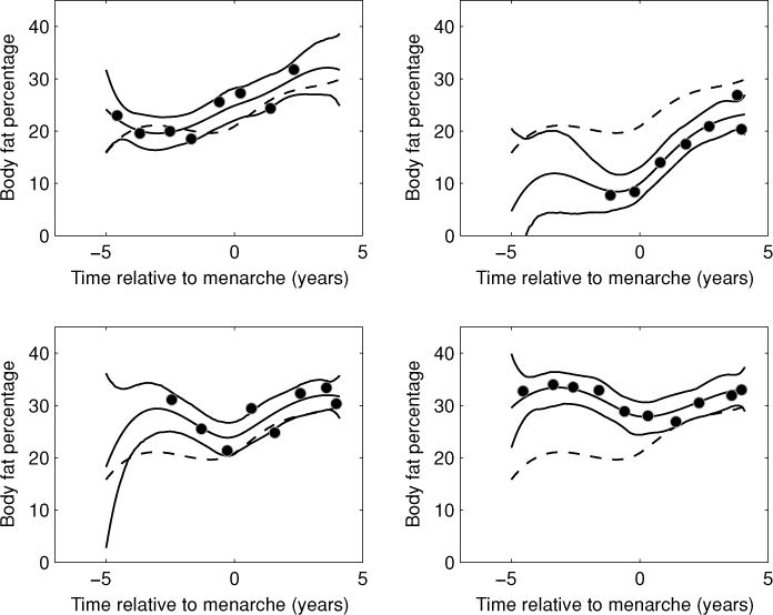
Estimated individual trajectories with 95% posterior credible intervals for four girls. Circles indicate actual data points and dashed lines indicate overall mean trajectory.
We explore the major modes of variation in body fat trajectories by performing an eigenanalysis of the within-individual covariance of the smoothed functions (James et al., 2001). The covariance function estimated using (9) is pictured in Figure 3, along with the corresponding correlation function. Within-girl correlation is fairly high across all time points; for example, the correlation between body fat percentages at 4 years premenarche and body fat percentages 3 years postmenarche is approximately 0.7. The covariance function shows higher variability in premenarche body fat percentages, with a gradual decrease postmenarche.
Figure 3.
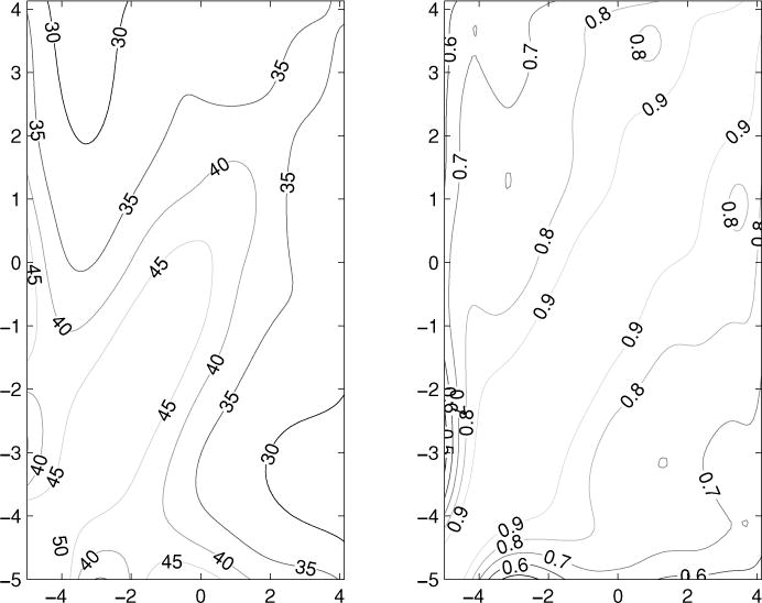
Left-hand panel: Contours of the covariance function for the body fat data. Right-hand panel: The corresponding correlation function.
The first two eigenfunctions of the covariance function are pictured in the left-hand panel of Figure 4. The first eigenfunction, accounting for almost 81% of the individual variation from the mean in the smoothed functional outcomes, describes sustained deviation from the mean over the entire time course of the study. The second eigenfunction, accounting for 8% of the smoothed variation, describes individual variation from the mean which peaks at about 3 years premenarche and again at approximately 2 years postmenarche but with an opposite sign. These eigenfunctions can also be used to identify individual curves which are unusual with respect to typical patterns of large-scale variation from the mean. For example, the right-hand panel of Figure 4 shows the two girls who had the largest positive scores corresponding to the projection of the individual functions onto the two eigenfunctions.
Figure 4.
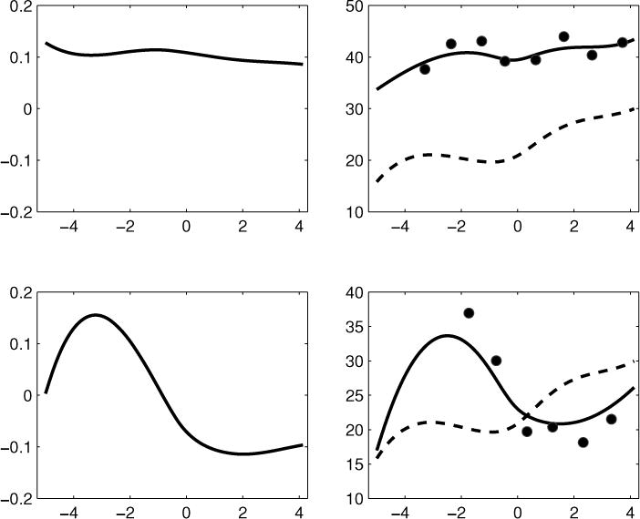
Top left-hand panel: The first eigenfunction of the covariance function of the body fat data. Bottom left-hand panel: The second eigenfunction of the covariance function. Top right-hand panel: The estimated individual trajectory (solid line) and actual data (circles) of the girl with the highest score on the first eigenfunction; the overall mean trajectory (dashed line) is provided for reference. Bottom right-hand panel: The same for the girl with the highest score on the second eigenfunction.
As a referee pointed out, the results of this analysis must be interpreted carefully, in that age at menarche is not accounted for. Age at menarche may be associated with the shape of body fat trajectories centered at time of menarche. One way of accounting for age at menarche would be to include it as a continuous predictor in a functional linear model. While we do not do this here, we indicate one way of doing this in Section 7.
6. Simulation Study
In this section, we evaluate the proposed methodology by performing a small simulation study. In the study, 100 data sets were generated from the model
| (10) |
Here, the Xi are ni × 7 design matrices of B-splines with interior breakpoints given by {0.2, 0.4, 0.6, 0.8} and evaluated at time values on the unit interval. The number of observations ni for a given individual was distributed as Poisson(6)+2; thus, a minimum of two and a mean of eight observations per individual curve were generated. The time points ti conditional on ni were uniformly distributed on the unit interval. The errors εi were generated as independent normals with zero mean and variance equal to 10. The random effects were generated as i.i.d. variates from an AR-1 model with mean β = (50, 70, −70, 70, 0, 20, 20)′ and correlation ρ = 0.9. The mean curve along with one simulated data set of 50 curves is pictured in the left-hand panel of Figure 5. The true within-individual covariance surface of the error-free (smooth) curves is pictured in the right-hand panel of Figure 5.
Figure 5.
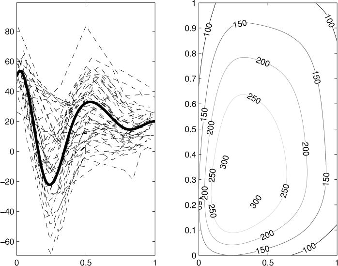
Left-hand panel: True mean trajectory (heavy solid line) and “observed” data from one realization of (10). Right-hand panel: Contours of true covariance function of noise-free curves simulated from (10).
For each data set, a pool of 30 equally spaced interior breakpoints was specified, and the beta prior on π was set to give an a priori expected number of 10 breakpoints with standard deviation 5. Other hyperparameters were set to the same values used in the example presented in Section 5. The sampling procedure of Section 4 was used on each data set to produce 10,000 iterates with a burn-in period of 2000. Nominal pointwise 95% credible intervals were evaluated on a fine grid for each of the 100 simulated data sets. The left-hand panel of Figure 6 plots the proportion of times that these posterior credible intervals contained the true mean curve. Over all time points, the true mean curve was contained within the intervals 96% of the time, with a minimum coverage of 91% and a maximum coverage of 100% across individual time points. Figure 6 (right-hand panel) also plots the average posterior probabilities of breakpoint inclusion for all 100 simulated data sets. The posterior probabilities of the indicator variables are highest in the regions of high curvature (with a maximum of 66%) and lowest in regions of low curvature.
Figure 6.
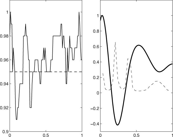
Left-hand panel: Estimated coverage probabilities for the pointwise nominal 95% posterior credible intervals from 100 data sets simulated from (10). Credible intervals and posterior coverage probabilities were computed at 100 equally spaced time points on the unit interval. The dashed line at 0.95 is included for reference. Right-hand panel: True mean curve (solid line) scaled to fit the plot, and average posterior probabilities of breakpoint inclusion (dashed line) for all 100 data sets simulated from (10).
7. Discussion
In this article, we have proposed a Bayesian model for sparse functional data. Most methodologies proposed to date for fitting sparse functional data have separate model selection and model fitting stages. Usually, the process is to select the “best” model according to some criterion and then estimate the model parameters conditional on this best model. This type of procedure can be computationally very expensive; for example, with only 10 breakpoints there are 210 possible models to select from. Another disadvantage of these approaches is that inferences on model parameters are also conditional on the best model selected. Because this ignores any uncertainty in the number and placement of breakpoints, these inferences may be unrealistically optimistic. Furthermore, inferences on model parameters also typically require further computational effort, usually some type of bootstrapping procedure.
In contrast, the Bayesian model and sampling scheme that we have proposed in this article unify model selection, model fitting, and posterior inferences into one procedure. With latent indicator variables for breakpoint inclusion, model selection becomes an integral part of the model estimation procedure. Thus, model selection uncertainty is automatically included in the estimates of posterior means for other model parameters. Most other procedures which also implement a Bayesian method for determining the level of smoothing for sparse functional data put constraints on the covariance kernel and are not locally adaptive. In contrast, our procedure has no such constraints and is locally adaptive.
One potential drawback of our proposed method is that it selects the same basis functions for the overall mean curve and for each of the individual curves. This implies that all individual trajectories have the same underlying level of smoothness. In the sparse functional data setting, it is not generally feasible to use our method to select basis functions (breakpoints) for each individual curve separately.
Some aspects of this model could benefit from further development. For example, extending the model to include discrete and continuous covariates would be desirable. One approach to do so follows along the lines of Guo (2002). Let xi and zi be p × 1 and q × 1 vectors of covariates, respectively. Then, similar to Guo (2002) and Morris and Carroll (2006), we could generalize model (2) to include these covariates as follows:
where Br(t) is a vector of B-spline basis functions for the rth covariate xir (evaluated at time t) with the corresponding vector of fixed effects βr, and As(t) is a vector of B-spline basis functions for the sth covariate zis with corresponding random effects asi. This model reduces to (2) if xi = zi = 1 and Br = Ar. Breakpoint selection might be identical for all covariates or might be accomplished separately for each covariate. The latter, for example, would allow for differing levels of smoothness or location of curve features across groups defined by levels of a categorical covariate.
Another area for future research is the theoretical development of the asymptotic performance of functional estimates and posterior inferences and the impact that the prior specification has on these. Finally, constructing simultaneous posterior credible regions within which the entire mean or individual trajectories are contained with given probability would be useful. One possibility is to construct a highest posterior density region for the entire function (Tanner, 1996) based on the posterior distribution of {b, β, Σb, γ}.
Supplementary Material
Acknowledgments
The first author was supported in part by NIH grant K25MH076981-01. The second author was supported in part by NSF grant DMS-0405038. Both authors were supported in part by RCMI grant 5G12 RR008124 from the NIH. We would also like to acknowledge the helpful comments of the editor, associate editor, and referees, which have resulted in a greatly improved article.
Footnotes
Supplementary Materials
The Web Appendix referenced in Section 4 is available under the Paper Information link at the Biometrics website http://www.tibs.org/biometrics. The data used here from MIT Growth and Development Study can be obtained from the website of Fitzmaurice et al. (2004) at http://biosun1.harvard.edu/fitzmaur/ala/.
Contributor Information
Wesley K. Thompson, Department of Statistics, University of Pittsburgh, Pittsburgh, Pennsylvania 15260, U.S.A
Ori Rosen, Department of Mathematical Sciences, University of Texas at El Paso, El Paso, Texas 79968, U.S.A.
References
- Bandini L, Must A, Spadano J, Dietz W. Relation of body composition, parental overweight, pubertal stage, and race-ethnicity to energy expenditure among premenarcheal girls. American Journal of Clinical Nutrition. 2002;76:1040–1047. doi: 10.1093/ajcn/76.5.1040. [DOI] [PubMed] [Google Scholar]
- Besse P, Ramsay J. Principal components analysis of sampled functions. Psychometrika. 1986;51:285–311. [Google Scholar]
- Bigelow J, Dunson D. (ISDS Discussion Paper 2005–06).Bayesian adaptive regression splines for hierarchical data. 2005a doi: 10.1111/j.1541-0420.2007.00761.x. [DOI] [PubMed] [Google Scholar]
- Bigelow J, Dunson D. (ISDS Discussion Paper 2005–18).Semiparametric classification in hierarchical functional data analysis. 2005b [Google Scholar]
- Brumback B, Rice J. Smoothing spline models for the analysis of nested and crossed samples of curves (with Discussion) Journal of the American Statistical Association. 1998;93:961–994. [Google Scholar]
- deBoor C. A Practical Guide to Splines, Revised Edition. New York: Springer-Verlag; 2001. [Google Scholar]
- Fitzmaurice G, Laird N, Ware J. Applied Longitudinal Data Analysis. Hoboken, New Jersey: Wiley; 2004. [Google Scholar]
- Guo W. Functional mixed effects models. Biometrics. 2002;58:121–128. doi: 10.1111/j.0006-341x.2002.00121.x. [DOI] [PubMed] [Google Scholar]
- Holmes C, Mallick B. Bayesian regression with multivariate linear splines. Journal of the Royal Statistical Society, Series B. 2001;63:3–17. [Google Scholar]
- Hoover D, Rice J, Wu C, Yang L. Nonparametric smoothing estimates of time-varying coefficient models with longitudinal data. Biometrika. 1998;85:809–822. [Google Scholar]
- James G, Sugar C. Clustering for sparsely-sampled functional data. Journal of the American Statistical Association. 2003;98:397–408. [Google Scholar]
- James G, Hastie T, Sugar C. Principal component models for sparse functional data. Biometrika. 2001;87:587–602. [Google Scholar]
- Kass R, Natarajan R. A default conjugate prior for variance components in generalized linear mixed models (Comment on an article by Browne and Draper) Bayesian Analysis. 2006;1:535–542. [Google Scholar]
- Kimmeldorf G, Wahba G. A correspondence between Bayesian estimation on stochastic processes and smoothing by splines. Annals of Mathematical Statistics. 1970;41:551–570. [Google Scholar]
- Kohn R, Smith M, Chan D. Nonparametric regression using linear combinations of basis functions. Statistics and Computing. 2001;11:313–322. [Google Scholar]
- Morris J, Carroll R. Wavelet-based functional mixed models. Journal of the Royal Statistical Society, Series B. 2006;68:179–199. doi: 10.1111/j.1467-9868.2006.00539.x. [DOI] [PMC free article] [PubMed] [Google Scholar]
- Müller H. Functional modeling and classification of longitudinal data (with Discussion and Rejoinder) Scandinavian Journal of Statistics. 2005;32:223–246. [Google Scholar]
- Phillips S, Bandini L, Compton D, Naumova E, Must A. A longitudinal comparison of body composition by total body water and bioelectrical impedance in adolescent girls. Journal of Nutrition. 2003;133:1419–1425. doi: 10.1093/jn/133.5.1419. [DOI] [PubMed] [Google Scholar]
- Ramsay J, Dalzell C. Some tools for functional data analysis (with Discussion) Journal of the Royal Statistical Society, Series B. 1991;53:539–572. [Google Scholar]
- Ramsay J, Silverman B. Functional Data Analysis. New York: Springer-Verlag; 1997. [Google Scholar]
- Ramsay J, Silverman B. Functional Data Analysis. 2nd. New York: Springer-Verlag; 2002. [Google Scholar]
- Rao C. Some statistical methods for the comparison of growth curves. Biometrics. 1958;14:1–17. [Google Scholar]
- Rice J. Functional and longitudinal data analysis: Perspectives on smoothing. Statistica Sinica. 2004;14:631–648. [Google Scholar]
- Rice J, Silverman B. Estimating the mean and covariance structure nonparametrically when the data are curves. Journal of the Royal Statistical Society, Series B. 1991;53:233–243. [Google Scholar]
- Rice J, Wu C. Nonparametric mixed effects models for unequally sampled noisy curves. Biometrics. 2000;57:253–259. doi: 10.1111/j.0006-341x.2001.00253.x. [DOI] [PubMed] [Google Scholar]
- Shi M, Weiss R, Taylor J. An analysis of paediatric CD4 counts for Acquired Immune Deficiency Syndrome using flexible random curves. Applied Statistics. 1996;45:151–163. [Google Scholar]
- Smith M, Kohn R. Nonparametric regression via Bayesian variable selection. Journal of Econometrics. 1996;75:317–344. [Google Scholar]
- Tanner M. Some Tools for Statistical Inference. New York: Springer-Verlag; 1996. [Google Scholar]
- Wang Y. Mixed effects smoothing spline analysis of variance. Journal of the Royal Statistical Society, Series B. 1998;60:159–174. [Google Scholar]
Associated Data
This section collects any data citations, data availability statements, or supplementary materials included in this article.