Abstract
Manifold-valued data arises frequently in medical imaging, surface modeling, computational biology, and computer vision, among many others. The aim of this paper is to introduce a conditional local distance correlation measure for characterizing a nonlinear association between manifold-valued data, denoted by X, and a set of variables (e.g., diagnosis), denoted by Y, conditional on the other set of variables (e.g., gender and age), denoted by Z. Our nonlinear association measure is solely based on the distance of the space that X, Y, and Z are resided, avoiding both specifying any parametric distribution and link function and projecting data to local tangent planes. It can be easily extended to the case when both X and Y are manifold-valued data. We develop a computationally fast estimation procedure to calculate such nonlinear association measure. Moreover, we use a bootstrap method to determine its asymptotic distribution and p-value in order to test a key hypothesis of conditional independence. Simulation studies and a real data analysis are used to evaluate the finite sample properties of our methods.
Keywords: Manifold-valued, Local distance correlation, Shape statistics
1 Introduction
Manifold-valued data frequently arises in many domains, such as medical imaging, computational biology, and computer vision, among many others [2, 23, 28, 11, 19]. Examples of manifold-valued data in medical imaging analysis include the Grassmann manifold, planar shapes, matrix Lie groups, deformation field, symmetric positive definite (SPD) matrices, and the shape representation of cortical and subcortical structures. Most manifold-valued objects are inherently non-linear and high-dimensional (or even infinite-dimensional), so analysis of these complex objects presents many mathematical and computational challenges.
Motivated by shape analysis, the aim of this paper is to measure a linear/nonlinear association between manifold-valued data (e.g., shape representation) and a random vector/variable (e.g., diagnosis), while controlling for the other random vector (e.g., age). Specifically, consider n independent observations {(Xi, Yi, Zi)}1≤i≤n, where Xi, Yi, and Zi are elements in metric spaces , , and , respectively. In traditional statistics, these metric spaces are Euclidean spaces of arbitrary dimension. Correlation and regression analyses are the fundamental statistic techniques for quantifying the degree of association between X and Y, with/without the effect of a set of controlling random variables Z removed. For instance, Pearson correlation and its multivariate extension, so-called canonical correlation analysis (CCA), are powerful tools for measuring the degree of linear association between X and Y. Moreover, partial correlation measures the degree of linear association between two random variables, while controlling for a random vector. Alternatively, one may fit a regression with Yi as response and both Xi and Zi as covariates such that , where β0, βx, and βz are regression coefficients and εi are measurement errors.
Generalizations of correlation and regression analyses to manifold-valued data are recently gaining popularity. Most existing methods for manifold-valued data are primarily on their mean and variation [5, 6, 10, 12]. Some nonparametric methods were subsequently developed for the density estimation of manifold data [3, 19, 21]. Recently, in [14], a Riemannian CCA model was proposed to measure an intrinsically linear association between manifold-valued data and a random vector (or two manifold-valued objects). Furthermore, various intrinsic regression models have been developed for manifold-valued data [13, 3, 4, 16, 24, 29, 7, 2, 19, 10, 9]. Most of these regression methods often require specifying a link function, projecting manifold-valued data to local tangent planes for computing residuals, and transporting all residuals to a common space [7].
However, when Xi or/and Yi are manifold-valued data, little has been done on the analysis of X and Y, while controlling for Z due to at least two major challenges. First, it is computationally challenging to optimize the objective function for the regression analysis of X and Y, when the dimension of X is relatively high. Such objective function is generally not convex and has a large number of parameters. Particularly, standard gradient-based optimization methods used in the literature strongly depend on the starting value of unknown parameters. Second, most intrinsic regression models for manifold-valued data require the specification of link functions (e.g., geodesic link), but it is conceptually challenging to choose a correct appropriate link function for any regression model that provides goodness of fit to a given data set. Due to these challenges, it is difficult to make further statistical inference (e.g., hypothesis test).
We propose a conditional local distance correlation to measure the nonlinear association between X and Y, while controlling for Z. Since such distance correlation measure solely requires the specification of the distances on the metric spaces , , and , it is applicable when both X and Y are manifold-valued data in different spaces. It also enjoys four major advantages. First, it avoids the optimization of a complex objective function, since empirical distance correlation measure is the function of pairwise distance between sample points. Second, it avoids the projection of manifold-valued data to local tangent planes. Third, it has a high statistical power of detecting complex and unknown nonlinear relationships between X and Y. Fourth, it is easy to make statistical inference on the nonlinear association between X and Y, while controlling for Z.
2 Methods
2.1 Conditional local distance correlation
We review a novel distance correlation for characterizing statistical dependence between two random variables or two random vectors of arbitrary dimensions [25]. In [15], distance correlation was further extended to stochastic processes in metric spaces when such metric spaces are of strong negative type. Distance correlation as an extension of Pearson correlation has several important properties. The first and most important one is that it is zero if and only if two random vectors are independent. The second one is its computational simplicity, since empirical distance correlation is the function of pairwise distance between sample points.
We introduce a conditional local distance correlation to measure the nonlinear association between X and Y, while controlling for Z, when , , and are metric spaces. Let dX(·,|·), dY (·, ·), and dZ(·, ·) be, respectively, the metrics of , , and . Let M( |Z) (or·M( |Z denote the set of finite conditional probability measures on (or ) given Z. We say that μ ∈ M( | Z) has a finite first moment if . we for some o ∈ Similarly, we can define ν ∈ ( | Z). Define aμ (x| z):= ∫dX(x, x′)dμ(x′|z) and DX(μ|z):= ∫dX(x, x′)dμ(x′|z)dμ(x|z) as finite functions when μ ∈ M|( |Z) has a finite first moment. Also, we can define av (y |z) DY (ν|z) for ν ∈ M( |Z) and Y.
Definition 1
The local distance covariance between random processes X and Y with finite moments given Z is defined as the square root of
where X′ and Y′ are the independent copies of X and Y, respectively.
By setting X = Y, we obtain the local distance variance as
Definition 2
The local distance correlation between random processes X and Y with finite moments given Z is defined as the square root of
if , or 0 otherwise.
Under the condition that the metric spaces are of strong negative type, it can be shown that if and only if X and Y given Z = z are conditionally independent. This property distinguishes the local distance correlation from the existing methods in the literature [14, 13, 3, 4, 16, 24, 29, 7, 2, 19, 7]. As shown below, it is easy to estimate and use its estimate to make statistical inference.
2.2 Estimation procedure
The next interesting question is to estimate the local distance covariance and correlation. The local distance dependence statistics are defined as follows. Let (Xi, Yi, Zi) for i = 1,…,n be a random sample of n independent and identically distributed random vectors from the joint distribution of random vectors (X, Y, Z). We compute two distance matrices (akl) = dX(Xk, Xl) and (bkl) = dY (Yk, Yl). For notational simplicity, it is assumed that holds. We consider a kernel function K(·) on Rr and the bandwidth h satisfying two regularity conditions as follows:
-
(C1)
, , , , and
-
(C2)
hr → 0, nhr → ∞, as n → ∞
Let ωh,k(Z) = Kh(Z − Zk), ωh,kl(Z) = Kh(Z − Zk)Kh(Z − Zl), ωh,ijkl(Z) = Kh(Z − Zi)Kh(Z − Zj)Kh(Z − Zk)Kh(Z − Zl), and , where Kh(Z) = K((Z − Zk)/h)/hr. We then introduce Akl(Z; h) as follows:
where akl = dX(Xk, Xl), , , and
Similarly, we can define bkl = dY (Yk, Yl) and Bkl(Z; h). Then, the empirical local distance covariance can be defined as
We define the empirical local distance correlation as
where
2.3 Inference procedure
The next question is to make statistical inference based on LDV or LDC. Our inference procedure consists of carrying out hypothesis test and constructing confidence interval.
To test the dependence of X and Y at a fixed location Z = z, we formulate it as follows:
| (1) |
We calculate the p–value of by using a local bootstrap procedure [18, 25, 26] as follows:
- Generate from {X1,…,Xn} with the probability
for j = 1,…,n. Then, we compute by using the local bootstrap sample . - Select a resampling number S, say 1,000. Repeat Step (i) S times and obtain for s = 1,…,S. And then the p-value of the test is given by
Given a confidence level α, we construct simultaneous confidence bands for as follows:
where and are the lower and upper limits of simultaneous confidence band, respectively. We use a bootstrap method to approximate the bounds:
- Resample from {(Xk, Yk, Zk): k = 1,…,n} with the probability
for j = 1,…,n, then compute by the bootstrap sample . Repeat Step (I) with resampling number S times and obtain And then the simultaneous confidence band is given by the quantiles at α and 1 − α of .
Like many other smoothing-based method, the performance of the proposed method depends upon the bandwidth h. It is widely acknowledged that the optimal h for nonparametric estimation is generally not optimal for testing. Selecting h to achieve optimal statistical power for (1) is an open problem. In practice, h can not be too large, since the conditional local distance covariance tends to the unconditional one. That is, an inappropriately large bandwidth h will yield a much larger false positive rate when X and Y are dependent. For simplicity, we consider the bandwidth h to eliminate the effect of Z on X and Y in the maximum extent. That is, the bandwidth h is chosen to minimize the mean of local distance covariance at every location Z = z. The intuition for the choice of h comes from partial correlation, whose aim is to eliminate the effect of Z on X and Y by the regression of Z on X and Y.
3 Numerical Studies
3.1 Simulations
We use two simulation studies to examine the finite sample performance of LDC. We consider the directional data on the unit sphere Rp, which denoted by for, both X and Y. Under the canonical Riemannian metric on Sp−1 induced by the canonical inner product on Rp, the geodesic distance between any two points X and X′ is equal to dX(X, X′) = arccos(XT X′). The sample size is set to be n = 300 and 400 in order to examine the finite sample performance of local distance estimate. We calculate the rejection rate at the significance level α = 0.05 and S = 200. Moreover, 200 replications are used for each simulation setting.
Simulation 1
We set p = 3 and consider the spherical coordinate of S2, denoted as (r, θ, ϕ), where r ∈ [0, ∞), θ ∈ [0, 2π], and ϕ ∈ [0, π], respectively, represent the radial distance, inclination (or elevation), and azimuth. The simulation datasets {(Xi, Yi, Zi) ∈ S2×S2×R: i = 1,…,n} were generated as follows:
-
(I.1)
, , and ;
-
(I.2)
, , and ;
-
(I.3)
, , and ;
-
(I.4)
Half of samples (Z ∼ U(−π+0.5, 0)) are generated from (I.2) and the other half (Z ∼ U(0, π−0.5)) are from (I.3);
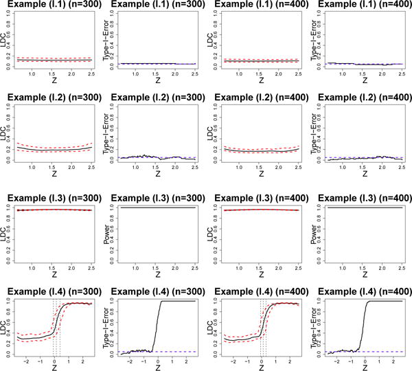
where , , , and were independently simulated from the Uniform distribution U(−π, π) and the εi, , and were independently simulated from the normal distribution N(0, 0.2). Therefore, X and Y are independent in (I.1), whereas they are dependent in (I.2) and (I.3). In contrast, X and Y are conditionally independent given Z in (I.1) and (I.2), whereas they are conditionally dependent in (I.3). For (I.4), the first half of samples are conditionally independent and the second half of samples are conditionally dependent given Z.
Figure 1 presents the estimated LDCs between X and Y given Z and their p-values. The Type I error rates based on the local bootstrap procedure are well maintained under the prefixed significance level, while the power of rejecting the null hypothesis is good. As the sample size n increases, simultaneous confidence bands become narrower and the value of local distance correlation is close to zero under the true conditional independence. We use the function e.cp3o in R package ecp to detect the change point of local distance correlation in (I.4). The estimated change point is very close to the true value of change point.
Fig. 1.

Figures of local distance correlation (95% confidence bands) and Type-I-Error/Power for n = 300 and n = 400 in simulation 1.
Simulation 2
We consider the von Mises-Fisher distribution, of which the data can be spherical or hyper-spherical. A p-dimensional unit random vector is set to be p-variate von Mises-Fisher distribution Mp(μ, κ). We set p = 10 and simulated μ from the multivariate normal distribution N(0, I10). The simulated datasets were generated as follows:
-
(II.1)
Xi ∼ M10(μx, 15), Yi ∼ M10(μy, 15), and Zi ∼ N(0, 0.5);
-
(II.2)
and , where , , and ξi = (u1 Zi…,u10 Zi), in which Zi ~ U(−1, 1) and with equal probability. Then, we project Xi and Yi to the unit spherical surface;
-
(II.3)
Xi ∼ M10(μx, 15), Yi = RXi, and Zi ∼ N(0,0.5) where R is a rotation matrix along the direction μx of μy
-
(II.4)
Half of samples (Z ~ U(−5, 0) were generated from (II.1) and the other half (Z ~ U(0, 5) were from (II.3).
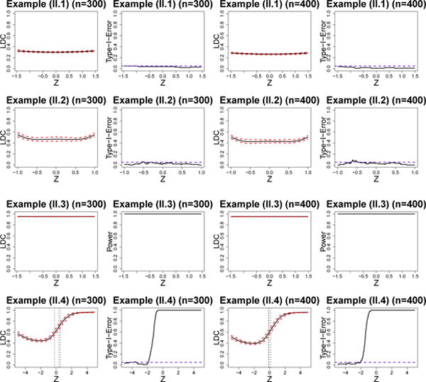
Similar to Simulation 1, X and Y are independent in (II.1), whereas they are dependent in (II.2) and (II.3). However, X and Y are conditionally independent given Z in (II.1) and (II.2), while they are conditionally dependent given Z in (II.3). The first half of samples are conditionally independent and the second half of samples are conditionally dependent given Z in (II.4). Inspecting Figure 2 reveals that the proposed methods work well.
Fig. 2.

Figures of local distance correlation (95% confidence bands) and Type-I-Error/Power for n = 300 and n = 400 in simulation 2.
3.2 Real Data Analysis
Alzheimer disease (AD) is a disorder of cognitive and behavioral impairment that markedly interferes with social and occupational functioning. It is an irreversible and progressive brain disease that slowly destroys memory and thinking skills, and eventually even the ability to carry out the simplest tasks. AD affects almost 50% of those over the age of 85 and is the sixth leading cause of death in the United States. The corpus callosum (CC), the largest white matter structure in the brain, has been a structure of high interest in many neuroimaging studies of neuro-developmental pathology. It contains homotopic and heterotopic interhemispheric connections and is essential for communication between the two cerebral hemispheres. Individual differences in CC and their possible implications regarding interhemispheric connectivity have been investigated in last several decades [27, 20].
We consider the CC contour data of the ADNI1 study. We processed the CC shape data for each subject in the ADNI1 study as follows. We used FreeSurfer package [8] to process each T1-weighted MRI, whereas the midsagittal CC area was calculated in the CCseg package.
We are interested in characterizing the change of the CC contour shape and its association with several key covariates of interest, such as age and diagnosis. We focused on n = 409 subjects with 223 healthy controls (HCs) and 186 AD patients at baseline of the ADNI1 study. Each subject has a CC planar contour Yi with 50 landmarks and nine covariates, including gender, age, handedness, marital status (Widowed, Divorced, and Never married), education length, retirement, and diagnosis. The demographic information is shown in Table 1. We treat the CC planar contour Yi as a manifold-valued response in the Kendall planar shape space and all covariates in the Euclidean space.
Table 1.
Demographic information for all participants.
| Disease status | Number of subjects | Age (years) | Females/males |
|---|---|---|---|
| Healthy control | 223 | 62–90 (76.25) | 107/116 |
| AD | 186 | 55–92 (75.42) | 88/98 |
The first scientific question of interest is to characterize the relationship between CC shape data and each of the nine covariates. Table 2 presents the distance correlation statistics for correlating CC data with each of the nine covariates. It reveals that the shape of CC planar contour are highly dependent on gender, education length, age and AD diagnosis at the significant level α = 0.05. It may indicate that gender, age and AD diagnosis are the most significant influence factors of CC planar contour, which agree with [1, 17, 22].
Table 2.
The distance correlation (Dcor) statistics for correlating CC contour data and nine covariates. The significance level is 0.05.
| covariates | Dcor | P–value |
|---|---|---|
| Gender | 0.186 | 0.001 |
| Handedness | 0.094 | 0.420 |
| Marital Status | 0.108 | 0.383 |
| Education length | 0.166 | 0.010 |
| Retirement | 0.108 | 0.165 |
| Age | 0.245 | 0.001 |
| Diagnosis | 0.190 | 0.001 |
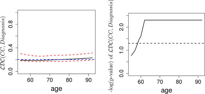
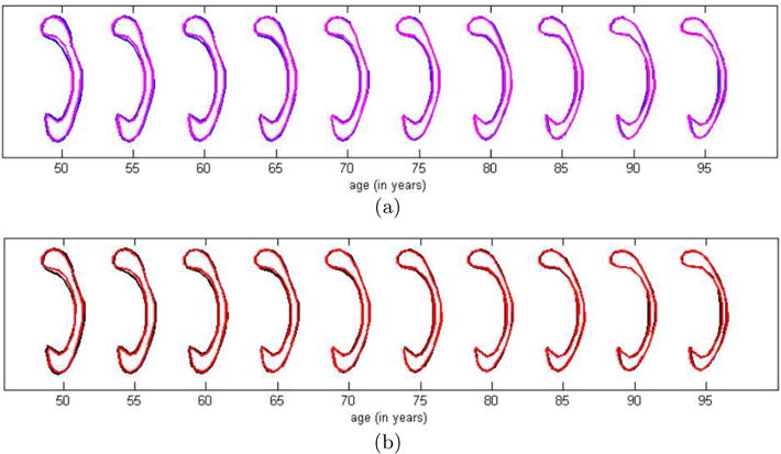
The second scientific question of interest is to characterize the relationship between CC shape data and AD diagnosis given age. Figure 3 presents the conditional local distance correlation of CC planar contour and AD diagnosis given age as a function of age. As age increases, the value of the conditional local distance correlation increases. It implies that diagnosis and CC are dependent with each other as age changes. Figure 4 presents the mean age-dependent CC trajectories for healthy controls and AD within each gender group. It can be observed that there is a major difference of the shape between the AD disease and healthy both in male and female groups. The splenium seems to be less thinner and the isthmus is rounded in subjects with AD disease than in healthy controls.
Fig. 3.

Figures of estimated local distance correlation and the corresponding negative log10(p-values) between CC planar contour and Diagnosis given Age.
Fig. 4.

ADNI data: Mean trajectories within each gender group: (a) female group (blue - normal; magenta - AD); (b) male group (black - normal; red - AD)
4 Conclusion
We proposed a local distance correlation for modeling data with manifold valued responses and applied this method to a variety of applications, such as the responses restricted to the sphere, shape spaces. The proposed method can detect complex nonlinear relationship and keeps the computational simplicity. In future, we will further investigate the theoretical properties of the new method and other applications in imaging analysis.
References
- 1.Allen LS, Richey M, Chai YM, Gorski RA. Sex differences in the corpus callosum of the living human being. The Journal of Neuroscience. 1991;11(4):933–942. doi: 10.1523/JNEUROSCI.11-04-00933.1991. [DOI] [PMC free article] [PubMed] [Google Scholar]
- 2.Banerjee M, Chakraborty R, Ofori E, Okun MS, Viallancourt DE, Vemuri BC. A nonlinear regression technique for manifold valued data with applications to medical image analysis. Proceedings of the IEEE Conference on Computer Vision and Pattern Recognition. 2016:4424–4432. [Google Scholar]
- 3.Bhattacharya A, Dunson DB. Nonparametric bayesian density estimation on manifolds with applications to planar shapes. Biometrika. 2010;97(4):851–865. doi: 10.1093/biomet/asq044. [DOI] [PMC free article] [PubMed] [Google Scholar]
- 4.Bhattacharya A, Dunson DB. Nonparametric bayes classification and hypothesis testing on manifolds. Journal of Multivariate Analysis. 2012;111:1. doi: 10.1016/j.jmva.2012.02.020. [DOI] [PMC free article] [PubMed] [Google Scholar]
- 5.Bhattacharya R, Patrangenaru V. Large sample theory of intrinsic and extrinsic sample means on manifolds-i. Annals of Statistics. 2003;31(1):1–29. [Google Scholar]
- 6.Bhattacharya R, Patrangenaru V. Large sample theory of intrinsic and extrinsic sample means on manifolds-ii. Annals of Statistics. 2005;33(3):1225–1259. [Google Scholar]
- 7.Cornea E, Zhu H, Kim PT, Ibrahim JG. Regression models on riemannian symmetric spaces. Journal of The Royal Statistical Society Series B-statistical Methodology. 2016 doi: 10.1111/rssb.12169. [DOI] [PMC free article] [PubMed] [Google Scholar]
- 8.Dale AM, Fischl B, Sereno MI. Cortical surface-based analysis. i. segmentation and surface reconstruction. NeuroImage. 1999;9(2):179–194. doi: 10.1006/nimg.1998.0395. [DOI] [PubMed] [Google Scholar]
- 9.Davis B, Fletcher PT, Bullitt E, Joshi S. Population shape regression from random design data. 2007:1–7. [Google Scholar]
- 10.Fletcher PT, Lu C, Pizer SM, Joshi S. Principal geodesic analysis for the study of nonlinear statistics of shape. IEEE Transactions on Medical Imaging. 2004;23(8):995–1005. doi: 10.1109/TMI.2004.831793. [DOI] [PubMed] [Google Scholar]
- 11.Grenander U, Miller MI. Pattern Theory From Representation to Inference. Oxford University Press; 2007. [Google Scholar]
- 12.Huckemann S, Hotz T, Munk A. Intrinsic manova for riemannian manifolds with an application to kendall’s space of planar shapes. IEEE Transactions on Pattern Analysis and Machine Intelligence. 2010;32(4):593–603. doi: 10.1109/TPAMI.2009.117. [DOI] [PubMed] [Google Scholar]
- 13.Kent JT. The fisher-bingham distribution on the sphere. Journal of the Royal Statistical Society. Series B (Methodological) 1982:71–80. [Google Scholar]
- 14.Kim HJ, Adluru N, Bendlin BB, Johnson SC, Vemuri BC, Singh V. European Conference on Computer Vision. Springer; 2014. Canonical correlation analysis on riemannian manifolds and its applications; pp. 251–267. [DOI] [PMC free article] [PubMed] [Google Scholar]
- 15.Lyons R. Distance covariance in metric spaces. The Annals of Probability. 2013;41(5):3284–3305. [Google Scholar]
- 16.Machado L, Leite FS, Krakowski K. Higher-order smoothing splines versus least squares problems on riemannian manifolds. Journal of Dynamical and Control Systems. 2010;16(1):121–148. [Google Scholar]
- 17.Ota M, Obata T, Akine Y, Ito H, Ikehira H, Asada T, Suhara T. Age-related degeneration of corpus callosum measured with diffusion tensor imaging. NeuroImage. 2006;31(4):1445–1452. doi: 10.1016/j.neuroimage.2006.02.008. [DOI] [PubMed] [Google Scholar]
- 18.Paparoditis E, Politis D. The local bootstrap for kernel estimators under general dependence conditions. Annals of the Institute of Statistical Mathematics. 2000;52(1):139–159. [Google Scholar]
- 19.Patrangenaru V, Ellingson L. Nonparametric Statistics on Manifolds and Their Applications to Object Data Analysis. CRC Press; 2015. [Google Scholar]
- 20.Paul LK, Brown WS, Adolphs R, Tyszka JM, Richards LJ, Mukherjee P, Sherr EH. Agenesis of the corpus callosum: genetic, developmental and functional aspects of connectivity. Nature Reviews Neuroscience. 2007;8(4):287–299. doi: 10.1038/nrn2107. [DOI] [PubMed] [Google Scholar]
- 21.Pelletier B. Kernel density estimation on riemannian manifolds. Statistics & Probability Letters. 2005;73(3):297–304. [Google Scholar]
- 22.Shuyu L, Fang P, Xiangqi H, Li D, Tianzi J. Shape analysis of the corpus callosum in alzheimer’s disease. 2007:1095–1098. [Google Scholar]
- 23.Srivastava A, Klassen EP. Functional and shape data analysis. Springer; 2016. [Google Scholar]
- 24.Su J, Dryden IL, Klassen E, Le H, Srivastava A. Fitting smoothing splines to time-indexed, noisy points on nonlinear manifolds. Image and Vision Computing. 2012;30(6):428–442. [Google Scholar]
- 25.Székely G, Rizzo M, Bakirov N. Measuring and testing dependence by correlation of distances. The Annals of Statistics. 2007;35(6):2769–2794. [Google Scholar]
- 26.Wang X, Pan W, Hu W, Tian Y, Zhang H. Conditional distance correlation. Journal of the American Statistical Association. 2016;110(512):1726. doi: 10.1080/01621459.2014.993081. [DOI] [PMC free article] [PubMed] [Google Scholar]
- 27.Witelson SF. Hand and sex differences in the isthmus and genu of the human corpus callosum. a postmortem morphological study. Brain. 1989;112(3):799–835. doi: 10.1093/brain/112.3.799. [DOI] [PubMed] [Google Scholar]
- 28.Younes L. Shapes and Diffeomorphisms. Springer; 2010. [Google Scholar]
- 29.Yuan Y, Zhu H, Lin W, Marron JS. Local polynomial regression for symmetric positive definite matrices. Journal of The Royal Statistical Society Series B-statistical Methodology. 2012;74(4):697–719. doi: 10.1111/j.1467-9868.2011.01022.x. [DOI] [PMC free article] [PubMed] [Google Scholar]


