Constrained Mixed-Effect Models with Ensemble Learning for Prediction of Nitrogen Oxides Concentrations at High Spatiotemporal Resolution

Abstract

Spatiotemporal models to estimate ambient exposures at high spatiotemporal resolutions are crucial in large-scale air pollution epidemiological studies that follow participants over extended periods. Previous models typically rely on central-site monitoring data and/or covered short periods, limiting their applications to long-term cohort studies. Here we developed a spatiotemporal model that can reliably predict nitrogen oxide concentrations with a high spatiotemporal resolution over a long time span (>20 years). Leveraging the spatially extensive highly clustered exposure data from short-term measurement campaigns across 1–2 years and long-term central site monitoring in 1992–2013, we developed an integrated mixed-effect model with uncertainty estimates. Our statistical model incorporated nonlinear and spatial effects to reduce bias. Identified important predictors included temporal basis predictors, traffic indicators, population density, and subcounty-level mean pollutant concentrations. Substantial spatial autocorrelation (11–13%) was observed between neighboring communities. Ensemble learning and constrained optimization were used to enhance reliability of estimation over a large metropolitan area and a long period. The ensemble predictions of biweekly concentrations resulted in an R² of 0.85 (RMSE: 4.7 ppb) for NO₂ and 0.86 (RMSE: 13.4 ppb) for NO_x. Ensemble learning and constrained optimization generated stable time series, which notably improved the results compared with those from initial mixed-effects models.

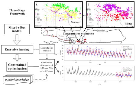
Graphical abstract

1. INTRODUCTION

Exposure to air pollution is associated with acute and chronic adverse health outcomes, such as respiratory and cardiovascular morbidity.^1,2 Spatiotemporal models that optimally characterize the environment are crucial to estimate exposures to ambient air pollutants with high spatiotemporal resolutions for large-scale epidemiologic studies. However, obtaining reliable estimates of long-term exposures relies on spatiotemporal models that fully capture complex temporal structure (e.g., both short and long-term temporal trends) jointly with multiscale spatial variations (e.g., regional- and local-scale spatial variations). Developing such spatiotemporal models is challenging because measurement data are limited in space and time, and complex, and nonlinear associations exist between predictors (such as meteorological and traffic variables) and pollutant concentrations.³

Many earlier studies used land-use regression or conventional kriging approaches to develop individual spatial models of exposure that capture details across space but not time. Such conventional approaches tend to overfit irregularities of the training data relying on a set of assumptions,^4,5 including having access to an unbiased sample of monitoring sites for the population and homogeneity of spatial variation for kriging. When the temporal variability of exposure is ignored in the modeling process, especially when statistical assumptions are violated, the resulting exposure estimates could be affected by large error causing significant biases or large variance.^6,7

In more recent years,^3,8–12 air pollution exposure modelers started to employ the variants of principal components called empirical orthogonal functions (EOFs)¹¹ for spatiotemporal modeling of air pollutants. In the approach, the first and second principal components accounting for the dominant temporal structure often explain the majority of the long-term and seasonal but not the short-term temporal pollutant variation in the study region. Two of these studies parametrized the temporal basis functions by incorporating time-invariant spatial variables such as elevation, distance to the shorelines and meteorological factors.^3,12 However, this two-stage approach generally assumes spatial-temporal independence and is limited in capturing short-term temporal variability in its estimates.

Other methods such as Bayesian maximum entropy have been used to estimate the spatiotemporal concentrations of particulate matter <10 µm (PM₁₀),¹³ particulate matter <2.5 µm (PM_2.5),¹⁴ and ozone.^15,16 Hierarchical spatiotemporal models have also been developed for PM with a second-order stationary and isotropic assumptions of spatiotemporal covariance.⁸ However, these methods were based on simulated variograms derived from limited measurement data subject to overfitting biases, and both methods only incorporated spatiotemporal covariates predictive of the means structure to a limited extent.

Here, we developed a novel spatiotemporal modeling framework to estimate nitrogen dioxide (NO₂) and nitrogen oxides (NO_x) at a high spatiotemporal resolution over a period of 22 years (1992–2013) using extensive data from government routine monitoring networks and rich short-term field sampling campaigns. Routine monitoring data were used to construct the temporal basis functions and to capture long-term and seasonal temporal trends of pollutants in the study region. The short-term samples from three monitoring field campaigns provided neighborhood scale spatial data that better captured intraurban spatial variability and spatial autocorrelation than the models trained just using the routine monitoring data. The modeling framework consisted of three stages: a generalized additive mixed model to capture spatiotemporal variability and spatial autocorrelation at a high resolution, ensemble learning of the mixed models to reduce uncertainty and to better characterize variability in prediction, and constrained optimization to ensure physically- and chemically consistent prediction of concentrations.

2. MATERIALS AND METHODS

2.1. Study Domain

This study region (Supporting Information (SI) Figure S1) covers the area of southern California south of the 35.6 degree latitude (~Bakersfield) and includes Los Angeles, Orange, Riverside, Ventura, Santa Barbara, Mohave, San Diego, Imperial Counties and most of San Luis Obispo, Kern, and San Bernardino Counties.

2.2. NO₂ and NO_x Measurements

Routine measurements of hourly NO₂ and NO_x concentrations from 1992 to 2013, recorded at 51 stations, were retrieved from ambient air monitoring networks operated by the California Air Resources Board, South Coast Air Quality Management District (SCAQMD), San Diego Air Pollution Control District (APCD), Antelope Valley AQMD, Mojave Desert AQMD, Imperial County APCD, San Joaquin Valley APCD, San Luis Obispo County APCD, Santa Barbara County APCD, and Ventura County APCD. The concentrations at these stations were measured using Federal reference (chemiluminescence NO/NO₂/NO_x) methods.

Additional data were generated in intensive field measurement campaigns conducted by the University of Southern California (USC), University of California Los Angeles (UCLA), and University of California Irvine (UCI), respectively. Passive diffusion-based Ogawa samplers¹⁷ were used to measure NO₂ and NO_x, with integrated biweekly samples for the USC and UCLA data and integrated weekly samples for the UCI data. The USC data were collected as part of the Intra-Community Variation campaigns conducted in 12 Children’s Health Study (CHS) communities in 2005–2006¹⁸ and eight CHS communities in 2008–2009¹⁹ (in total, 2,542 biweekly samples from 1,104 locations). The UCLA data contain 161 samples collected in Los Angeles County with two biweekly measures (i.e., September 16 to October 1, 2006 and February 10–25, 2007).²⁰ The UCI data contain 32 samples collected in south Los Angeles and Orange counties during 4 weeks (i.e., July 10–18, July 24 to August 1, November 13–21, and December 4–12 in 2009).²¹

Since most (about 97%) of the field measurements were integrated biweekly samples (mainly from USC and UCLA), we used biweekly averages as the temporal unit of estimation. For the routine measurements, biweekly average concentrations were calculated from hourly data using a 75% completeness criterion. For the field measurements, linear interpolation was used to derive biweekly averages from the UCI weekly data. For a site with a full temporal coverage, a total of 574 biweekly concentrations were calculated from January 1992 to December 2013.

Section 2 and Table S1 of SI provide more details about the measurements of NO₂ and NO_x and adjustment for the passive data from the field campaigns to minimize systematic bias. SI Figure S1 also shows the locations for the routine and USC sampling sites [the UCI and UCLA sampling locations concealed to comply with specific requirements by their Institutional Review Boards].

2.3. Spatiotemporal Covariates

2.3.1. Traffic-Related Covariates

2.3.1.1. CALINE4-Estimated Concentrations from Local Traffic Emissions

CALINE4 is a line source dispersion model that was used to assess the contribution of local motor vehicle emissions to ambient concentrations.^22,23 We used CALINE4 to compute mean NO_x concentrations from emissions respectively on freeways and nonfreeways. The time-varying NO_x estimates by CALINE4 were derived using the quarterly average daily traffic volumes and EMFAC2011 (for 1992–2012)²⁴ and EMFAC2014 (for 2013)²⁵ (see SI Section 3.1 for details).

2.3.1.2. Traffic Density

Traffic density represents distance-decayed annual average daily traffic (AADT) volume in both directions from all roads (freeways/highways and major surface streets) within a circular buffer. Its values were computed by the ESRI ArcGIS density function using a kernel with a 300 m search radius and a 5 m grid resolution. Due to covering a long time period, the traffic densities were scaled by the South Coast Air Basin (SoCAB) EMFAC2011 vehicle fleet average NO_x emission factor for 50 mph and 6% heavy-duty vehicle fraction to reflect the composite trend in traffic volumes and emissions over time (see SI Section 3.2 of see SI Section 3.2 for details).

2.3.1.3. Distance to Roadways

We calculated the distance from the sampling location to the centerline of the nearest roadway by road class based on the ERSI Premium Street Map road network data. The two directions of travel were represented as separate line segments for freeways and other moderate and high volume roads in this data set.

2.3.1.4. Population Density

We calculated block group population in 300 m buffers based on the 1990, 2000, and 2010 census block data in ArcGIS and linearly interpolated or extrapolated annual population density for 1992–2013 at the sampling sites.

2.3.2. Meteorological Covariates

Meteorological covariates were derived from a high-resolution (4-km) gridded data set of surface daily meteorological variables that cover the contiguous United States from 1979 to 2013.²⁶ Seven meteorological factors were extracted as predictive variables: minimum and maximum air temperatures (°C), specific humidity (grams of vapor per kilogram of air), precipitation (amount of rain per square meter in 1 h (millimeters, mm)), wind speed (meters/second), wind direction (degree), near-ultraviolet and near-infrared spectra (watt/meter², w/m²).

2.3.3. Elevation and Distance to Shoreline

We obtained high accuracy elevation (at 30 m resolution) data using GoogleMap API²⁷ for each sampling location. We also calculated the shortest distance (meter) to the shoreline of the Pacific Ocean for each sampling location.

3. MODELING APPROACH

We designed a hierarchical modeling framework (Figure 1) with three stages: a mixed-effect spatiotemporal model, ensemble learning, and constrained optimization.

Figure 1.

Modeling framework for estimation of the spatiotemporal concentrations of NO₂ and NO_x.

3.1. Stage 1: Mixed-Effect Model to Capture Spatiotemporal Variability of Pollutant Concentrations

We designed the mixed-effect model that incorporated nonlinear relationships, fixed and random effects from multiple predictors, and spatial autocorrelation to characterize spatiotemporal variability of NO₂ and NO_x concentrations.

The spatiotemporal estimate (f(s,t)) of the concentrations of NO₂ and NO_x is quantified using the following formula:

$$f(s,t)={\beta }_0+s(f_1(t))+s(f_2(t))+f_r(s,t)+\sum _{i=1}^{k}s(x_i(s,t))+f_s(r_s)+f_{\mathit{\text{re}}}(r_s)+\epsilon$$ (1)

where s refers to spatial location, t refers to temporal parameter, β₀ represents the long-term mean concentration, f₁(t) and f₂(t) are temporal basis functions that represent long-term and seasonal trends, f_r(s,t) represents annual regional variation in pollution where regions are defined as the Thiessen polygons derived from the government routine monitoring stations, x_i(s,t) represents local variability explained by different local predictors (e.g., CALINE4 estimates, traffic density, population density and meteorological parameters), f_s(r_s) represents structured spatial effects (r_s refers to the region where s is located), f_re(r_s) represents unstructured spatial effects, and ε represents the residuals.

The seasonal effects (f₁(t) and f₂(t)) reflect the long-term dominant temporal trend for the study region. We used the empirical orthogonal functions (EOFs) (a.k.a., independent temporal basis functions) and the long-term biweekly concentrations from the 51 routine monitoring stations to derive the dominant basis functions. EOFs were used to present leading modes of spatiotemporal variability of air pollution; their smoothed curves are often used to reduce noise due to random fluctuation.¹¹

We used the yearly average pollutant concentrations for each Thiessen polygon (f_r(s,t)) surrounding each routine monitoring station to reflect the regional yearly spatial variability (fixed effect in the model). Thiessen polygons are often used to determine density of point samples and to build meshes for space-discretized analyses.²⁸ Spatiotemporal variability due to local effects (x_i(s,t)) was modeled using variables that influence air pollutant dispersion or reflect the type and strength of emission sources, including meteorological parameters, traffic-related variables, population density etc. Traffic-related variables and population density capture the influence of on-road mobile and area emission sources, whereas meteorological parameters mainly influence the environmental processes involved in air pollutant transport, dispersion and removal.

For spatiotemporal factors, we adopted a nonparametric additive method to model nonlinear effects (see SI Section 4.1 for details). Degrees of freedom were limited to 10 to minimize overfitting.

Better characterization of spatial-effect terms in the model development is important to account for the influence of neighboring polygons (spatial autocorrelation). In this study, we used structured spatial random effects to account for spatial autocorrelation not explained by spatial covariates. Additive unstructured random effects²⁹ were also included to account for spatial autocorrelation not fully explained by structured spatial random effects (e.g., other spatially distributed sources of pollutants besides traffic emission and population density). By estimating a structured component and an unstructured component, we can distinguish between the two sources of spatial autocorrelations.³⁰ Our empirical results showed that adding unstructured random effects slightly improved model performance (measured by the deviance information criterion) compared to the one with only structured random effects.

Thiessen polygons were constructed around the central points of the monitoring locations within a certain buffer distance to simulate spatial effects. By sensitivity analysis, a buffer distance of 500 m was selected as an optimal aggregate option due to its good balance between accuracy and computing efficiency. In our model, spatial effects were treated as random variables at the polygon level and incorporated formally as a component of the nonparametric additive terms.

Restricted maximum likelihood was used to solve the geo-additive mixed-effect model. We used the packages of BayesXsrc and BayesX to solve the mixed model^31,32 in the statistics software R (Version 3.3). SI Section 4.2 presents the formulas and details about modeling of spatial random effects.

3.2. Stage 2: Ensemble Learning to Reduce Uncertainty and Variability in Point Prediction

As Stage 2 of the modeling framework, we designed an algorithm of weighted bootstrap aggregation³³ for the spatiotemporal models to ensure stable prediction. This algorithm iteratively selected a random sample of size n (n = 18 096, size of the original training data set) with replacement, stratified by traffic index (traffic density and Caline4 estimated concentration), from the original data set, and 90% of the predictors for training. In each iteration, about 63% and 37% of the original data set were selected to train and test the model, respectively.³⁴ So, the final result was equivalent to a 63–37% cross validation. We also conducted a sensitivity analysis where only ²/₃ of the predictors were used each time and the resulting model performed slightly worse (R² decreased by about 4%) than when using 90% of the predictors. The selected samples were used to train multiple different models. The number of iterations (from 10 to 1,210 by a step of 20) was determined using cross-validation to minimize the root-mean-square error (RMSE). The aggregated predictions (mean and standard deviation) are the weighted means of the outputs of all trained models, where the weighting is the square of each model’s R² (see Section 4.3 for details).

Randomly sampling from both the training data set and the predictors was used to ensure independence between the training samples for different models. Given that each model was trained for different portions of the original data set, the variance in the predictions can be effectively decreased, as demonstrated in the literature of machine learning.^7,33 Besides the weighted predicted mean of concentration, the weighted standard deviation (SI eq S6) can be obtained, as an uncertainty indicator to reflect the dispersion of the predicted value.

3.3. Stage 3: Constrained Optimization to Help with Long-Term Continuous Time Series Estimation

Stage 2 generated averaged point estimates for specific-location and -time for which the full set of predictors was available. However, the predictors, especially the time-varying covariates, may be temporally incomplete for the entire modeling period. For locations with a large portion of incomplete time-varying covariates, the predictions from Stage 2 might not fully capture the dominant seasonal trend. Thus, as Stage 3 of the modeling framework, we designed constrained optimization to derive optimal coefficients for the temporal basis functions [f₁(t) and f₂(t) in eq 1)]. While the temporal basis functions represented the principle components of temporal variability for the study region, their coefficients reflected spatial difference in the long term averages and seasonal variation between different locations. Using the basis functions with their coefficients, the full time series of concentrations covering the study period can be simulated for a target location in the study region. Then, the corresponding time-specific estimates could be extracted from the simulated series as adjusted values for the estimates of Stage 2. In constrained optimization, the point estimates from Stage 2 were employed to estimate the coefficients of the temporal basis functions (β₀, β₁, and β₂). Such optimization was solved through quadratic programming.

The constrained optimization aims to minimize the difference between the target concentration to be adjusted and the prediction output from Stage 2 subject to certain constraint conditions.

$${\text{min}}_{{\beta }_i(i=0,1,2)}=1/2\sum _{s,t}{(y_{\mathit{\text{st}}}-{\hat{y}}_{\mathit{\text{st}}})}^2$$ (7)

$${\hat{y}}_{\mathit{\text{st}}}={\beta }_0(s)+{\beta }_1(s)f_1(t)+{\beta }_2(s)f_2(t)$$ (8)

where y_st is the measurement and/or estimate derived from ensemble learning in Stage 2, f₁(t) and f₂(t) are the temporal basis functions, and β₀, β₁ and β₂ are the coefficients of the temporal basis functions to construct the time series of the concentration over the entire study period.

The following constraints were designed according to a priori and empirical knowledge,^5,35,36 and implemented:

Constraints:

1. β_{0 lower} ≤ β₀ ≤ β_{0 upper} to control the long-term mean and limit extreme values in prediction;

2. β_{1 lower} ≤ β₁ ≤ 0 to control the seasonal trends (higher in winter and lower in summer);

3. β_{2 lower} ≤ β₂ ≤ β_{2 upper} to control the scale of seasonal variation;

4. β₁(f₁(t) − f₁(t + Δt)) + β₂(f₂t) − f₂(t + Δt)) ≥ 0 to control the decreasing trend in concentrations for the study domain, where Δt is the difference in time between the start year (t) and the end year (t+Δt); In this study, we used a start year of 1993 and an end year of 2013.

5. NO₂(β₀(s) + β₁(s)f₁(t) + β₂(s)f₂(t)) < NO_x(β₀(s) + β₁(s)f₁(t) + β₂(s)f₂(t)) to ensure that NO₂ predictions are smaller than or equal to NO_x.

6. β₀(s) + β₁(s)f₁(t) + β₂(s)f₂(t) ≤ L_max to control the maximum concentration (L_max) for NO₂ and NO_x.

The intervals (β_{i lower} or β_{i upper}) of the beta parameters were determined from the long-term time series of measurements at routine monitoring stations (using outer fence³⁷ to filter the outliers) and used to constrain the target functions to get stable seasonal trends.

3.4. Validation

3.4.1. Validation for Individual Models

Prediction errors, R-square (R²), RMSE, relative RMSE [NRMSE = normalized RMSE = RMSE/(y_max − y_min), and CV RMSE = coefficient of variation of the RMSD= RMSE/ӯ] were used to evaluate the individual models. To assess prediction error, residual plots were also examined for evidence of over- /under-fitting and heteroscedasticity. Leave-one-subcounty-out cross validations were conducted. In this validation, all samples within one subcounty were held out as the validation data while keeping the remaining data from the other subcounties to train the model, and then this resulting model was used to make prediction for the held-out samples in the subcounties not used to train the model. The goal of leave-one-subcounty-out cross validation was to examine the model’s performance across different sub counties using independent training data set.

Since one important application of the model is to estimate NO₂ and NO_x exposure for the subjects residing in the CHS communities, we also conducted leave-one-community-out cross validation specifically for the CHS samples. The CHS monitoring locations were highly clustered in space within each community, which created challenges in reliably estimating concentrations at individual sites within certain communities. We also examined the model performance for each individual CHS community.

3.4.2. Validation of the Output by Ensemble Learning

In ensemble learning, using bootstrap aggregation, we employed about 63.2% of the original data set to train the model to make predictions for the remaining 36.8% of the data set. Similar performance measures (R², RMSE, relative RMSE) as used for the individual models were calculated using the output from ensemble learning for all samples and for field sampling campaign data separately.

3.4.3. Validation of Constrained Optimization

For constrained optimization, the Pearson’s correlation between the adjusted biweekly estimates obtained by constrained optimization and the observed values were respectively computed over the long-term study period for each routine monitoring station. Correlations from all routine monitoring sites then were summarized.

3.4.4. Application: Lifetime Exposure Estimation for Children’s Health Study Participants

We employed the trained spatiotemporal models to make predictions at the CHS subject locations across southern California. In total, we predicted 1 850 415 biweekly NO₂ and NO_x concentrations at 10 820 locations for 1992–2013, the time period covering the lifetime residential histories of CHS participants (5845 unique individuals in cohort E). Since one of the two major USC field campaigns occurred in 2005–2006, we obtained the averages for summer (June–August 2005) and winter (December 2005 to February 2006) of those years to create maps for visual checks of spatial and seasonal patterns of pollutant concentrations at subject locations.

4. RESULTS

4.1. Summary of Measured Concentrations

Table 1 lists the summary statistics of the concentrations and the sampling locations from routine monitors as well as field campaigns conducted by USC, UCLA, and UCI. The histograms (SI Figure S2) show small skewness for NO₂ and large skewness for NO_x; thus, we log-transformed NO_x to make its distribution more normal.

Table 1.

Summary of NO₂ and NO_x Measurements

		distribution of monitoring locations by data completeness (number of biweekly time periods with valid data)				mean concentration (ppb)
source	number of monitoring locations	≤100	(100,280]	(280,400]	>400	NO2	NOx	correlation between NO2 and NOx
agencies	51	9	13	7	22	24.3	45.7	0.81

			distribution of sampling locations by data completeness (number of biweekly time periods with valid data)					mean concentration (ppb)
source		number of sample locations	1	2	3	4	>5	NO2	NOx	correlation between NO2 and NOx
USC	ICV1a	987	41	570	376			16.5	36.7	0.85
	ICV2a	117	28	71	11	5	2	16.7	27.9	0.87
UCLA		184		184				24.6	56.7	0.84
UCI		32			14	18		18.1	33.2	0.88

^aICV: The Intra-Community Variability study.

4.2. Stage 1 Mixed-Effects Model

The temporal basis functions were used to capture the seasonal trend of pollutant concentrations for the study region (SI Figure S3). The first component of the temporal basis trend accounted for 59% of the variance for NO₂ and 56% of the variance for NO_x. The second temporal basis function explained a lower percentage of variance (about 9% for NO₂ and 8% for NO_x).

The selected local spatiotemporal variables made different contributions to the variance explained in the mixed model (SI Table S2 where the thresholds are also listed as the filter for the outliers). Among these factors, CALINE4 NO_x on freeways and traffic density (300 m-5 km) each accounted for 9–13% of the variance, and population density accounted for 5–11% of the variance. Wind speed and minimum air temperature together account for about 7–8% of the variance. The additive mixed models captured nonlinear associations between predictive variables and pollutant concentrations (SI Figure S4). Generally, traffic density, CALINE4 output and population density were positively and nonlinearly associated with pollutant concentrations.

The Thiessen polygons generated with the optimal 500 m radius were selected for modeling spatial effects (SI Figure S5).

The individual models from Stage 1 achieved an R² of 0.90 for NO₂ and 0.91 for NO_x (RMSE: 2.08 ppb for NO₂; 10.02 ppb for NO_x) with the leave-one-subcounty-out cross validation R² of 0.83 (RMSE: 5.39 ppb) for NO₂ and 0.88 for NO_x (RMSE 12.42 ppb) (Table 2). The leave-one-community-out validation specifically for the USC data shows an R² of 0.71 for NO₂ and 0.80 for NO_x with the RMSE of 4.51 ppb for NO₂ and 9.37 ppb for NO_x. The validation results for the CHS communities are presented in SI Table S3 and S4. While the total correlation between the predicted and observed values was 0.95 (RMSE: 2.54 for NO₂; 5.43 for NO_x), the model performance was not as good for CHS communities with the lowest NO₂ and NO_x concentrations: Lake Arrowhead and Santa Maria.

Table 2.

Validation for the Total Samples and the Field Campaign Samples

		pollutant	correlation	R2	RMSE (ppb)	NRMSE	CV RMSE
regular (all the data used to train the models)		NO2	0.95	0.90	2.08	0.02	0.09
		NOx	0.96	0.91	10.02	0.03	0.12
leave-one-subcounty- out cross validation		NO2	0.91	0.83	5.39	0.06	0.22
		NOx	0.94	0.88	12.42	0.04	0.27
ensemble learning validation	all the samples	NO2	0.92	0.85	4.70	0.05	0.20
		NOx	0.93	0.86	13.33	0.02	0.13
	USC, UCLA, and UCI samples	NO2	0.91	0.82	3.92	0.09	0.23
		NOx	0.94	0.88	8.12	0.06	0.21
	USC samples	NO2	0.91	0.83	3.80	0.09	0.23
		NOx	0.95	0.90	7.06	0.05	0.20
leave-one-community-out cross validation for USC samples		NO2	0.88	0.71	4.51	0.11	0.28
		NOx	0.91	0.80	9.37	0.07	0.26

4.3. Ensemble Learning and Constrained Optimization for Stable Prediction of Time Series

Through bootstrap aggregation, we obtained the optimal number (120) of individual mixed-effect models. For the total samples, validation results for the ensemble models showed similar accuracy as individual models (Table 2); for the field campaign samples, the ensemble learning generated better results, in particular showing considerable improvement (12% for NO₂; 10% for NO_x) for the USC samples, compared with the result of the leave-one-community-out cross validation (Table 2). The residual plots for ensemble predictions between the observed values vs residuals show slight overfitting and no heteroscedasticity (SI Figure S6). Figure 2 shows the residual plots of the ensemble predictions for the USC samples. We also examined R² and RMSE for each community of the USC samples; worse model performance was observed for several communities, that is, the Lake Arrowhead and Santa Maria, and Anaheim. The data (SI Figure S7) show that Lake Arrowhead and Santa Maria had the lowest concentrations of NO₂ and NO_x and thus the model slightly overestimated their concentrations, while Anaheim had the highest NO₂ concentrations and the model slightly underestimated NO₂.

Figure 2.

Plots of the residuals vs the observed values for the ensemble NO₂ (a) and NO_x (b) predictions at the USC sampling locations.

The validation for constrained optimization shows a strong correlation between the simulated time series and the observed values. The mean and median of Pearson’s correlations between the simulated time series and observed values for each routine monitoring station are respectively 0.94 for NO₂ (0.96 for NO_x) and 0.97 for NO₂ (0.99 for NO_x) (SI Figure S8 for the boxplot). Even for the sites with the lowest correlation (0.55 for NO₂; 0.7 for NO_x), the simulated temporal trends were basically consistent with the observed values (SI Figure S9).

Figure 3 presents the plots of observed vs predicted values with the simulated time series generated by constrained optimization for one typical monitoring station. Even for the sample locations with many missing observed values (e.g., with only 4–5 measurements available for the USC sample locations), our approach can capture the basic temporal trends over the long-term period. The summer (June to August of 2004) vs winter (December 2004 to February 2005) average concentration estimates highlight local scale spatial variations with a general declining trend further away from heavily traveled roads, and higher concentration in winter than in summer. Contrast and gradient variations were also observed within the communities (e.g., Anaheim for NO₂ in Figure 3; and San Dimas for NO_x in SI Figure S10).

Figure 3.

Observed vs predicted values, and simulated series of NO₂ (a) and NO_x (b) for a test location in West Los Angeles (shown as the yellow five-pointed star in SI Figure S1).

5. DISCUSSION

In this study, we developed a novel hierarchical modeling framework to make robust predictions for spatiotemporal concentrations of NO₂ and NO_x over 22 years. Our spatiotemporal model improved over the previous two-stage model approaches^3,9,12 that only separated the temporal variability (characterized by temporal basis functions) from the spatial variability (modeled exclusively by spatial variables), but did not make full use of the spatiotemporal variables (e.g., meteorological variables were averaged over the entire study period and treated solely as spatial variables). In the two-stage models, the first two temporal basis functions and their coefficients (estimated by spatial covariates) were used as the dominant predictors. In the two-stage framework, the model’s performance in prediction was limited by the total variance that can be accounted for by the selected temporal basis functions (e.g., only 68% for NO₂ and 64% for NO_x in the case of this study). Further, the two-stage models assumed that temporal and spatial variances are distinctly separable. In practice, it is often difficult to completely separate the two. Such separation may result in loss of information on temporal variability in predictors and consequently substantial uncertainty in prediction. In this study, we developed a flexible three-stage framework with multiple features to improve model prediction. First, a nonlinear mixed model was developed to best capture both regional and local, as well as long-term and short-term variability in pollutant concentrations in a single model. Then, ensemble learning and constrained optimization were implemented to reduce uncertainty, minimize variance in prediction, and generate stable predictions.

The mixed model has a flexible framework making it easy to incorporate multiple spatiotemporal predictors and spatial effects. For instance, the model incorporated long-term average concentrations (intercept), long-term seasonal trends (the first and second temporal basis functions), regional variation in concentration (subcounty-level yearly averages) and local-scale influential predictors. At this stage, the temporal basis functions and associated coefficients are not the sole basis for the model’s framework but rather used to represent long-term seasonal variation predictors for the study region.

Local variability in the environmental processes (e.g., emission, transport, dispersion, and removal), was represented in our air pollution model by spatiotemporal covariates including traffic indicators, population density, and meteorological factors. In terms of traffic indicators, the CALINE4 and traffic density predictors incorporated quarterly or annual variations in traffic volumes, emission, and wind, which was important to capture temporal variation and trends in local on-road vehicle emissions. These two predictors accounted for a significant proportion of the variances, illustrating influence of traffic emissions on concentrations of NO₂ and NO_x. Population density, an indirect measure of emissions, explained 5–11% variance. In comparison, the meteorological parameters together accounted for 7–8% of spatiotemporal variability, although CALINE4 also captured part of the meteorological impact.

Nonlinear models were fit to account for local variability. Such models captured the critical points where different trends occurred. For example, in SI Figure S4-a and b, the increase in concentrations with traffic density was more rapid for traffic density below 50 than that above 50. Comparisons between linear and nonlinear models show that the nonlinear model improved the variance explained by about 19–21%.

In this study, we used Thiessen polygons rather than point-based kriging to model spatial autocorrelation. An assumption of kriging is random and even distribution of sample points with homogeneity of spatial variation.^38,39 For this study, many sampling points from USC were highly clustered and thus not applicable for kriging. Thiessen polygons remained relatively stable regardless of the density of samples and distribution of spatial variation, and are effective in capturing neighborhood scale spatial variability. Spatial autocorrelation accounted for a significant portion of the variance.

Most previous exposure models^4,40,41 used single data sets to fit a single model that was then evaluated using cross validation. The primary drawback of the single learner model, like our mixed-effect model in Stage 1, is that the model may overfit the training data and be variable when applied to new locations and times with their predictors different from the primary range of the training data set. In comparison, the ensemble learner combines individual predictions from different models, and thus it minimizes variation in prediction.^42,43 In this study, we trained different mixed models using multiple sets of samples obtained by bootstrap aggregation with different combinations of prediction variables. The final prediction was determined by weighting all outputs of individual models by accuracy, and the standard deviations of the predictions were derived as uncertainty indicators. This approach reduces variance and enhances the reliability of prediction.

The leave-one-community-out cross validation shows a good predictive performance overall. The results varied by individual community, with better performance in communities with moderate pollution levels and relatively poor performance in the mountain communities with lower pollution levels, such as Lake Arrowhead. As expected, the model is not capable of accurately predicting the cases having the lower observed concentration than that of the samples used to train the model.

The coupling of constrained optimization with the temporal basis functions is useful to simulate reliable long-term time series. The constrained optimization leveraged a priori and empirical knowledge (e.g., concentration of NO₂ lower than that of NO_x, declining trends for NO₂ and NO_x over the long period, and seasonal variation) and a limited number of point estimates to have an optimal estimation of the parameters for the temporal basis functions, thus extrapolating the concentrations far (1992–2013) from our denser measurement campaigns in 2005 or later. This approach is particularly useful for situations where long-term time series of exposures are needed but the subject locations have incomplete predictor variables (e.g., USC sample locations).

This study employed unbalanced sampling data that included routine measurement data and short-term field campaign measurements. Ideally, one would rely on high spatiotemporal resolution measurements (i.e., frequent measurements over the whole period of 22 years and across the entire study region). However, a number of our short-term samples were spatially clustered. To address this concern regarding clustered data, we made strict leave-one-subcounty-out and leave-one-community-out cross validations to test the model’s actual performance and the results were satisfactory (R²: 0.83–0.88). By subsequent ensemble learning and constrained optimization to decrease bias, the final predictions at CHS subject locations (Figure 4 and SI Figure S10) showed fine concentration gradients within each community, illustrating the model’s capability to estimate within-community variability.

Figure 4.

Average predicted NO₂ in summer (a) and winter (b) in 2005–2006 at USC ICV1 sampling locations in Anaheim, Orange County.

The study has several limitations. First, this is a model of NO₂/NO_x from traffic pollution since the traffic-related predictors such as CALINE4 NO_x and traffic density were used, not a model for prediction of airport or shipping or other stationary combustion sources. For the latter, we need the extra covariates to capture the corresponding sources in the model. Second, there is a potential overfitting problem in the nonparametric nonlinear model. We limited the degrees of freedom (10) for the explanatory variables to decrease overfitting in generalized additive models. Ensemble learning further reduced overfitting. Third, not all of the short-term samples were carefully selected and sited for exposure modeling purposes. Since the USC data were highly clustered, more Thiessen polygons were constructed at these locations with a denser sample, which may result in better spatial resolution for these locations than that for the sparse sample (e.g., overestimation in Lake Arrowhead). Although our method can be applied to different situations (sparse vs dense sampling), when additional samples become available, these can be used to update the model for continual improvement. Fifth, the study region is confined to southern California and 1992–2013 calendar years only, but the modeling approach is easily generalizable to other regions and periods.

References

- 1.Zanobetti A, Schwartz J, Samoli E, Gryparis A, Touloumi G, Peacock J, Anderson HR, Tertre LA, Bobros J, Celko M, Goren A, Forsberg B, Michelozzi P, Rabczenko D, Hoyos PS, Wichmann EH, Katsouyanni K. The temporal pattern of respiratory and heart disease mortability in response to air pollution. Environ. Health Perspect. 2003;111:1188–1193. doi: 10.1289/ehp.5712. [DOI] [PMC free article] [PubMed] [Google Scholar]
- 2.Mahiyuddin W, Sahani M, Aripn R, Latif M, Thach T, Wong C. Short-term effects of daily air pollution on mortality. Atmos. Environ. 2013;65:69–79. [Google Scholar]
- 3.Szpiro AA, Sampson DP, Sheppard L, Lumley T, Adar DS, Kaufman DJ. Predicting intra-urban variation in air pollution concentrations with complex spatio-temporal dependencies. Environmetrics. 2010;21:606–631. doi: 10.1002/env.1014. [DOI] [PMC free article] [PubMed] [Google Scholar]
- 4.Hoek G, Beelen R, Hoogh K, Vienneau D, Gulliver J, Fischer P, Briggs D. A review of land-use regression models to assess spatial variation of outdoor air pollution. Atmos. Environ. 2008;42:7561–7578. [Google Scholar]
- 5.Jerrett M, Arain A, Kanaroglou P, Beckerman B, Potoglou D, Sahsuvaroglu T, Morrison J, Giovis C. A review and evaluation of intraurban air pollution exposure models. J. Exposure Anal. Environ. Epidemiol. 2005;15:185–204. doi: 10.1038/sj.jea.7500388. [DOI] [PubMed] [Google Scholar]
- 6.Eugene K. On the Algorithmic Implementation of Stochastic Discrimination. IEEE Trans. Pattern Anal. Mach. Intell. 2000;22:473–490. [Google Scholar]
- 7.Hastie T, Tibshirani R, Friedman JH. The Elements of Statistical Learning. Springer; New York: 2009. [Google Scholar]
- 8.Cameletti M, Ignaccolo R. Scientific Meeting of SIS, 45th Scientific meeting of Italian Statistical Society. University of Padua; 2010. Comparing spatio-temporal hierarchical models for air quality data. [Google Scholar]
- 9.Li LF, Wu J, Ghosh JK, Ritz B. Estimating spatiotemporal variability of ambient air pollutant concentrations with a hierarchical model. Atmos. Environ. 2013;71:54–63. doi: 10.1016/j.atmosenv.2013.01.038. [DOI] [PMC free article] [PubMed] [Google Scholar]
- 10.Christakos G, Serre M. BME analysis of spatiotemporal particulate matter distributions in North Carolina. Atmos. Environ. 2000;34:3393–3406. [Google Scholar]
- 11.Finkenstadt B, Held L, Isham V. Statistical Methods for Spatio-Temporal Systems. Chapman & Hall/CRC; New York: 2007. [Google Scholar]
- 12.Lindstrom J, Szpiro AA, Sampson DP, Sheppard L, Oron A, Richards M, Larson T. A Flexible Spatio-Temporal Model for Air Pollution: Allowing for Spatio-Temporal Covariates. University of Washington; Seattle: 2011. [DOI] [PMC free article] [PubMed] [Google Scholar]
- 13.Yu H, Chen J, Christakos G, Jerrett M. BME estimation of residential exposure to ambient PM10 and ozone at multiple time scales. Environ. Health Perspect. 2009;117:537–544. doi: 10.1289/ehp.0800089. [DOI] [PMC free article] [PubMed] [Google Scholar]
- 14.Yang Y, Christakos G. Spatiotemporal Characterization of Ambient PM2.5 Concentrations in Shandong Province (China) Environ. Sci. Technol. 2015;49:13431–8. doi: 10.1021/acs.est.5b03614. [DOI] [PubMed] [Google Scholar]
- 15.Adam-Poupart A, Brand A, Fournier M, Jerrett M, Smargiassi A. Spatiotemporal modeling of ozone levels in Quebec (Canada): a comparison of kriging, land-use regression (LUR), and combined Bayesian maximum entropy-LUR approaches. Environ. Health Perspect. 2014;122:970–6. doi: 10.1289/ehp.1306566. [DOI] [PMC free article] [PubMed] [Google Scholar]
- 16.de Nazelle A, Arunachalam S, Serre ML. Bayesian maximum entropy integration of ozone observations and model predictions: an application for attainment demonstration in North Carolina. Environ. Sci. Technol. 2010;44:5707–13. doi: 10.1021/es100228w. [DOI] [PMC free article] [PubMed] [Google Scholar]
- 17.Koutrakis P, Wolfson JM, Bunyaviroch A, Froehlich SA. Passive Ozone Sampler Based On A Reaction with Nitrite. Health Effects Institute; Boston, MA: 1994. pp. 19–47. [PubMed] [Google Scholar]
- 18.Franklin M, Vora H, Avol E, McConnell R, Lurmann F, Liu F, Penfold B, Berhane K, Gilliland F, Gauderman WJ. Predictors of intra-community variation in air quality. J. Exposure Sci. Environ. Epidemiol. 2012;22:135–47. doi: 10.1038/jes.2011.45. [DOI] [PMC free article] [PubMed] [Google Scholar]
- 19.Fruin S, Urman R, Lurmann F, McConnell R, Gauderman J, Rappaport E, Franklin M, Gilliland FD, Shafer M, Gorski P, Avol E. Spatial variation in particulate matter components over a large urban area. Atmos. Environ. 2014;83:211–219. doi: 10.1016/j.atmosenv.2013.10.063. [DOI] [PMC free article] [PubMed] [Google Scholar]
- 20.Su GJ, Jerrett M, Beckerman B, Wilhelm M, Ghosh KJ, Ritz B. Predicting traffic-related air pollution in Los Angeles using a distance decay regression selection strategy. Environ. Res. 2009;109:657–670. doi: 10.1016/j.envres.2009.06.001. [DOI] [PMC free article] [PubMed] [Google Scholar]
- 21.Li L, Wu J, Wilhelmc M, Ritz B. Use of generalized additive models and cokriging of spatial residuals to improve land-use regression estimates of nitrogen oxides in Southern California. Atmos. Environ. 2012;55:220–228. doi: 10.1016/j.atmosenv.2012.03.035. [DOI] [PMC free article] [PubMed] [Google Scholar]
- 22.Benson P. CALINE4: A Dispersion Model for Predicting Air Pollutant Concentrations near Roadways. California Department of Transportation; Sacramento, CA: 1989. [Google Scholar]
- 23.Wu J, Houston D, Lurmann F, Ong P, Winer A. Exposure of PM2.5 and EC from diesel and gasoline vehicles in communities near the Ports of Los Angeles and Long Beach, California. Atmos. Environ. 2009;43:1962–1971. [Google Scholar]
- 24.California Air Resources Board. EMFAC2011 Technical Document. 2011 [Google Scholar]
- 25.California Air Resources Board. EMFAC2014 Volume III-Technical Documentation. 2015 [Google Scholar]
- 26.Abatzoglou TJ. Development of gridded surface meteorological data for ecological applications and modelling. Int. J. Climatol. 2013;33:121–131. [Google Scholar]
- 27.Google GoogleAPI. https://developers.google.com/maps/
- 28.Seidel R. The upper bound theorem for polytopes: an easy proof of its asymptotic version. Comp. Geom. 1995;5:115–116. [Google Scholar]
- 29.Richard E, E C, S M. Statistical Methods for Trend Detection and Analysis in Environmental Science. 2011 [Google Scholar]
- 30.Besag J, York J, Mollié A. Bayesian image restoration with two applications in spatial statistics. Ann. I. Stat. Math. 1991;43:1–59. [Google Scholar]
- 31.Belitz C, Brezger A, Klein N, Kneib T, Lang S, Umlauf N. BayesX: Methodology Manual. 2015 [Google Scholar]
- 32.Zurr FA. Mixed Mixed Effects Models and Extensions in Ecology with R. Springer; New York: 2007. [Google Scholar]
- 33.Breiman L. Bagging predictors. Mach. Learn. 1996;24:123–140. [Google Scholar]
- 34.Aslam AJ, Popa RA, Rivest RL. Proceedings of the Electronic Voting Technology Workshop (EVT ’07), Boston, MA, 2007. Boston, MA: 2007. On Estimating the Size and Confidence of a Statistical Audit. [Google Scholar]
- 35.California Environmental Protection Agency. Review of the California Ambient Air Quality Standard For Nitrogen Dioxide. California Environmental Protection Agency; 2007. [Google Scholar]
- 36.Clean Air Technology Center (MD-12) Nitrogen Oxides (NOx), Why and How They Are Controlled. U.S. Environmental Protection Agency; NC: 1999. [Google Scholar]
- 37.NIST/SEMATECH. e-Handbook of Statistical Methods. 2016 [Google Scholar]
- 38.Goovaerts P. Geostatistics for Natural Resources Evaluation. Oxford University Press; New York: 1997. [Google Scholar]
- 39.Chiles PJ, Delfiner P. Geostatistics: Modeling Spatial Uncertainty. John Wiley & Sons; New York: 1999. [Google Scholar]
- 40.Hesterberg TW, Bunn WB, McClellan RO, Hamade AK, Long CM, Valberg PA. Critical review of the human data on short-term nitrogen dioxide (NO2) exposures: evidence for NO2 no-effect levels. Crit. Rev. Toxicol. 2009;39:743–781. doi: 10.3109/10408440903294945. [DOI] [PubMed] [Google Scholar]
- 41.Ryan PH, LeMasters GK. A review of land-use regression for characterizing intraurban air models pollution exposure. Inhalation Toxicol. 2007;19:127–133. doi: 10.1080/08958370701495998. [DOI] [PMC free article] [PubMed] [Google Scholar]
- 42.Dietterich TG. Workshop on Multiple Classifier Systems, 2000. Springer-Verlag; 2000. Ensemble Methods in Machine Learning; pp. 1–15. [Google Scholar]
- 43.Hoeting JA, Madigan D, Raftery AE, Volinsky CT. Bayesian model averaging: A tutorial (vol 14, pg 382, 1999) Stat. Sci. 2000;15:193–195. [Google Scholar]
Associated Data
This section collects any data citations, data availability statements, or supplementary materials included in this article.