

Abstract
Tasmanian devils face a combination of threats to persistence, including Devil Facial Tumor Disease (DFTD), an epidemic transmissible cancer. We used RAD sequencing to investigate genome-wide patterns of genetic diversity and geographic population structure. Consistent with previous results, we found very low genetic diversity in the species as a whole, and we detected two broad genetic clusters occupying the northwestern portion of the range, and the central and eastern portions. However, these two groups overlap across a broad geographic area, and differentiation between them is modest (FST = 0.1081). Our results refine the geographic extent of the zone of mixed ancestry and substructure within it, potentially informing management of genetic variation that existed in pre-diseased populations of the species. DFTD has spread across both genetic clusters, but recent evidence points to a genomic response to selection imposed by DFTD. Any allelic variation for resistance to DFTD may be able to spread across the devil population under selection by DFTD, and/or be present as standing variation in both genetic regions.
Keywords: conservation genomics, devil facial tumor disease, gene flow, population bottlenecks, RAD sequencing, transmissible cancer
Introduction
Species of conservation concern often face a combination of threats, such as loss of habitat, population fragmentation, environmental change, and disease. Genetic diversity is critical to persistence in the face of these threats to maintain population fitness and adaptive potential, including the ability to evolve resistance to emerging infectious diseases (Frankham 2005). Tasmanian devils (Sarcophilus harrisii), marsupial carnivores whose geographic range is restricted to the island of Tasmania, exhibit exceedingly low levels of species-wide genetic diversity as a result of several historical factors (Jones et al. 2004; Miller et al. 2011; Brüniche-Olsen et al. 2014). These factors include bottlenecks in the devil population at the end of the last glacial maximum and during the Mid-Holocene, which likely resulted from climatic fluctuations that limited food availability, and European settlement and bounty hunting (Brüniche-Olsen et al. 2014).
More recently, devils have experienced a dramatic population decline due to an emerging infectious disease, Devil Facial Tumor Disease (DFTD). This clonally transmissible cancer has led to a decrease in the total devil population of more than 85% in the last two decades, including local declines of more than 90% (Lachish et al. 2007; McCallum et al. 2007; Jones et al. 2008). First recorded in the northeastern corner of Tasmania in 1996, the disease has spread across most of the island with only a few known populations yet unaffected along the northwestern and southwestern coasts. Extinction has been predicted as a possible outcome (McCallum et al. 2009); however, most local populations have not completely disappeared. In fact, some populations have recently shown an increase in numbers for the first time since DFTD arrival, and there is evidence for a genomic response by the devil to selection imposed by the disease (Epstein et al. 2016). These results suggest the presence of genetic variation in devils for tolerance or resistance to DFTD, despite overall low levels of genetic diversity.
Understanding patterns of genetic diversity and identifying barriers to gene flow in devils are important for several reasons. Genetic patterns may inform epidemiological models of disease spread among devil populations, and may help predict how disease resistance alleles could respond to selection across the species range. An understanding of phylogeographic patterns of genetic diversity may also inform management actions, such as translocations or reintroductions, which may be warranted in response to DFTD, in addition to management of captive populations. Genetic diversity and population connectivity will strongly influence the ability of devils to adapt to other threats such as environmental change and anthropogenic disturbances.
Previous characterizations of genetic diversity and population structure in devils have focused on relatively few (<12) microsatellite loci (Jones et al. 2004; Brüniche-Olsen et al. 2014), MHC loci (Siddle et al. 2010), mitochondrial genomes (Miller et al. 2011), SNPs (Miller et al. 2011; Wright et al. 2015; Morris et al. 2015), or whole-genome sequencing of two individuals (Miller et al. 2011). Here we use Restriction-site-Associated DNA sequencing (RADseq) (Andrews et al. 2016) to identify and genotype a large number of polymorphic nuclear loci at 38 localities across the species range to assess genome-wide patterns of genetic diversity and population structure. Our findings largely agree with previous results showing low overall genetic diversity and two broad-scale genetic clusters, but we further refine the geographic patterns of genetic diversity within the broad zone of overlap between these clusters.
Materials and methods
Ear tissue biopsies were collected at 38 locations (1–2 individuals per site) between 1998 and 2009 (Fig. 1, Table S1). IRB approval was obtained for tissue collection (Washington State University Institutional Animal Care and Use Committee protocol ASAF #04392; see Hawkins et al. (2006) for trapping protocols). With the exception of a few sites close to the first DFTD appearance in the northeast, sites were free of disease or no longer than 4 years after disease discovery at that location at the time of sampling. DNA was extracted using Qiagen DNA extraction kits. We constructed single-digest RADseq libraries (Baird et al. 2008; Etter et al. 2011) for 72 individuals, with pstI as the restriction enzyme to target a relatively large number of loci. Twenty-four individuals were barcoded and multiplexed per lane, in 3 lanes of paired-end 150 bp reads using an Illumina HiSeq2500.
Fig. 1.
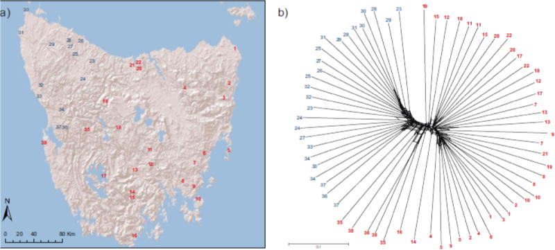
a) Map of Tasmania with localities of sampling sites. Each number represents a sampling site for one or two individuals (listed in Table S1). b) Neighbor-net consensus tree. Cluster assignment per individual based on STRUCTURE results is indicated by blue for the northwestern cluster and red for the central plateau and eastern coast cluster (see Fig. 2a). Scale bar represents uncorrected P distance. Numbers correspond to the map (Fig. 1a)
We de-multiplexed and filtered the reads with process_radtags from Stacks v1.20 (Catchen et al. 2013) using the default settings of the -q and –r options, which filter by read quality using a sliding window and rescue barcodes with up to 2 errors, respectively. We removed PCR duplicates with clone_filter, also from Stacks. Read pairs were aligned to the reference genome (Murchison et al. 2012) using bowtie2 (Langmead and Salzberg 2012) with the sensitive, end-to-end, and -X 900 options. Alignment files were processed using samtools (Langmead and Salzberg 2012) and we removed reads with a mapping quality < 40. To minimize variance in sequence coverage, from this point we retained only the forward reads (containing the restriction enzyme cut sites). We identified and genotyped single-nucleotide polymorphisms (SNPs) using the Stacks reference-aligned pipeline (pstacks, cstacks, sstacks, and populations). The default settings were used except for a minimum stack depth of 3 and the bounded error model with an upper bound of 0.1, to increase sensitivity to minor alleles when PCR duplicates have been removed (Catchen et al. 2013). We dropped two individuals with more than 95% missing data, and we further removed SNPs on the X chromosome, those with an observed heterozygosity greater than 0.5 (to eliminate confounded paralogs), those genotyped in less than one-half of the samples (35 samples), or those with alleles present in only one or two copies. We kept only one SNP per RAD locus to reduce linkage disequilibrium.
For individuals that passed quality filtering (N = 70), we calculated the number of segregating sites, mean coverage, Watterson’s θ (Watterson 1975) and Tajima’s D (Tajima 1989) using a custom python script. F-statistics were calculated using Genepop (Raymond and Rousset 1995). We tested for isolation by distance (IBD) with a Mantel test in the Vegan package (v.2.0-10; Oksanen et al. 2015) with 1000 permutations (alpha=0.05), using log10-transformed geographic distances and genetic distances, which were calculated in Genepop.
To identify genetic clusters, we used three different analyses. First, we inferred a phylogenetic network with the neighbor-net method in SplitsTree4 (v4.13.1; Huson and Bryant 2006), using uncorrected P distance. Second, we conducted a Bayesian model-based clustering using STRUCTURE v2.3.4 (Pritchard et al. 2000). We used the general admixture model without a priori assumptions about sample locations, and tested K = 1–10. Each K was run with 20 independent iterations, each with 500,000 Markov Chain Monte Carlo (MCMC) repetitions following a burn-in of 50,000. We estimated LnP(K) and ΔK using the Evanno method (Evanno et al. 2005) implemented in STRUCTURE HARVESTER (Earl and vonHoldt 2012) to obtain the most likely value of K. To combine the multiple iterations for each K, we used CLUMPAK (Kopelman et al. 2015). Third, we incorporated spatial information to inform individual ancestry estimates using TESS3 (Caye et al. 2016), which is useful in determining genetic barriers or genetic discontinuities in continuous populations. The default values of the program were implemented and each run was replicated five times. The optimal value of K corresponded to the minimum of the cross-entropy criterion, across the range K = 1–38.
Results
There were 175,274 putative RAD loci in the final filtered set, which resulted in 523,386 unfiltered putative SNPs. After all quality filters, RAD sequencing provided 6,362 SNPs. These SNPs were randomly distributed across the genome (Table S2), with 1,311 SNPs in genic regions based on the annotated reference genome (Ensembl Devil_ref v7.0). Mean coverage across individuals at genotyped loci was ~4.7X. Mean Watterson’s θ was 0.00013. The dataset did not deviate significantly from neutrality with a mean Tajima’s D value of 0.00019 across loci. Differentiation among all populations was relatively low, with FST = 0.1313 (95% CI: 0.1212 – 0.1392). We did not find a significant correlation between geographic and genetic distance across all individuals (Fig. S1; Mantel statistic r: 0.002719; p = 0.48052).
Our analyses were generally consistent with two major genetic clusters of Tasmanian devils, but with a broad geographically structured zone of admixture between them. The neighbor-net consensus tree grouped the northwestern populations together, and the Central Plateau and east coast populations together (Fig. 1b). However, there appear to be several sites intermediate to these two clusters, including those in the central-west region around Macquarie Harbor (sites 35–38 in Fig. 1), as well as broad-scale geographic structuring within each region. Similarly, STRUCTURE analysis showed populations in the northwest corner of the island are differentiated from the Central Plateau and east coast populations (Fig. 2a). K = 2 received the strongest support (Ln P(K) = −220483.4, ΔK = 1910.5; Table S3), and differentiation between these two clusters was FST = 0.1081 (95% CI: 0.1074 – 0.1082). However, there is a large degree of uncertainty in determining the optimal value of K (Pritchard et al. 2000; Evanno et al. 2005), and different values of K may reflect different demographic processes, so considering all K values with a biological interpretation is recommended (Meirmans 2015). Here, K = 3 and K = 4 (Figs. 2b–c) revealed a broad zone of admixture between the two groups. The TESS3 analysis did not support a best value of K, indicating fine population structure (the cross-entropy curve generated did not exhibit a clear plateau or change in curvature; Caye et al. 2016). The results show similar clustering as the STRUCTURE results when K = 2 with populations in the northwestern corner differentiated from all other populations (Fig. 2d). At higher values of K, south and central-west populations cluster together in K = 3 (Fig. 2e) and an additional Central Plateau cluster forms at K = 4 (Fig. 2f).
Fig. 2.
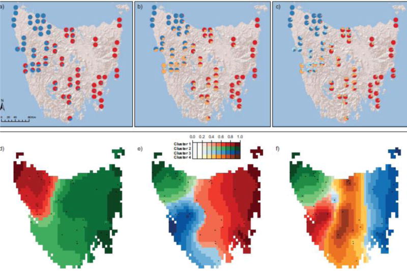
Population structure estimated using (a–c) STRUCTURE or (d–f) TESS3, based on 70 Tasmanian devil individuals across 38 sites with one to two individuals per site. (a–c) Pie charts indicate proportion of ancestry per individual; sites with two individuals appear as vertical pairs. (d–f) Colors indicate ancestry coefficients, and black dots show sampling localities. STRUCTURE showed maximum support for K = 2, while TESS3 did not support a best value of K, so here we show (a,d) K = 2, (b,e) K = 3, and (c,f) K = 4
Discussion
We found low genetic diversity throughout the devil geographic range, based on our estimate of Watterson’s θ, consistent with previous results (Jones et al. 2004; Lachish et al. 2010; Siddle et al. 2010; Miller et al. 2011; Brüniche-Olsen et al. 2014; Morris et al. 2015). Major periods of loss of genetic diversity resulting from population declines occurred at the last glacial maximum (~20 k years before present (YBP)) and during El Niño-Southern Oscillation climate cycles during the mid-Holocene (3–5 k YBP). Low genetic diversity predates the isolation of Tasmania from mainland Australia ~13k YBP (Brüniche-Olsen et al. 2014). Low genetic diversity may be a contributing factor to the rapid spread of DFTD and decline of devil populations (Morris et al. 2015).
Here, we confirmed previous evidence that northwestern populations are differentiated from the eastern populations (Miller et al. 2011; Brüniche-Olsen et al. 2014), potentially due to limited dispersal across unsuitable habitat, such as tall wet forest and alpine regions that separate the two areas. Miller et al. (2011) found differentiation between northwestern, central, and eastern coastal populations based on mitochondrial sequence data. Contrary to this clustering, Bruniche-Olsen et al. (2014) found that individuals from Macquarie Heads (western coast) differentiated from northwest populations with Central Plateau and east coast populations being admixed. Similarly, our analysis identified the Macquarie Heads individuals as the only pure representatives of a third population cluster when K = 3 (Fig. 2b).
While our data are consistent with two major genetic clusters, and K = 2 was best supported in STRUCTURE, our results from both STRUCTURE and the neighbor-net and TESS3 analyses also highlight the presence of finer-scale genetic structure that may be biologically important (Meirmans 2015). Finer-scale patterns of differentiation and admixture may reflect historical patterns of gene flow. Long distance dispersal (~110km) has been recorded in devils (Lachish et al. 2010), and our results suggest dispersal that has produced broad areas of admixture among genetic clusters. For instance, one individual from Lake Rowallan (site 19) genetically clusters with the eastern population (Figs. 1 and 2), suggesting the possibility of recent long-distance migration. Nonetheless, areas of admixture appear to be geographically well-defined, which would not be expected from frequent long-distance dispersal. It is worth noting that while the central-west and Central Plateau populations may be viewed as zones of admixture given our STRUCTURE results, that is not to say that they do not contain genetic variation that may be unique and important to adaptation (De Carvalho et al. 2010).
Implications for Conservation and Management
Assessing levels of genetic differentiation in future studies will continue to be important in managing both wild and captive populations. Despite genetic differentiation between eastern and western populations, DFTD has spread across this genetic boundary, indicating widespread genetic susceptibility. However, given decreased population density and dispersal distances due to disease (Lachish et al. 2010), population structure may increase in the future due to neutral processes. Our data largely reflect patterns of genetic diversity before the effects of disease on population genetic structure could occur, so they are informative to historic patterns of gene flow and pre-disease distribution of standing genetic variation. A recent study suggests that devils are experiencing a rapid evolutionary response to strong selection imposed by DFTD, likely acting on pre-disease standing variation, with the potential for evolution of resistance to the disease (Epstein et al. 2016). If variation for resistance is not lost due to decreased density and dispersal, resistance alleles may either already occur or spread throughout the population, allowing for range-wide evolution of resistance of DFTD. However, if disease resistance is linked to phylogeographic clusters and cannot spread across the range, artificial movements of animals among genetic clusters should be considered carefully to increase disease resistance, as well as overall genetic diversity across all loci (Frankham 2016).
Currently, the Tasmanian devil captive insurance population has individuals from the western side of the island and the north central coast (Hogg et al. 2015). To preserve all potential pre-bottleneck diversity detected in this study, future management practices may consider including individuals from the admixture zones of the central-west and Central Plateau (Fig. 2c,f). Given that our dataset provides a random sample of the genome, it integrates both neutral and adaptive variation. Including individuals from the admixture zones may maximize genetic diversity and preserve adaptive potential of devils to endure climate fluctuations or future disease epidemics, such as the recently discovered DFT2, a second appearance of transmissible cancer in devils (Pye et al. 2016). Such adaptive potential may rely not only on unique genetic variants, but also on unique multi-locus genotypes that can occur in admixed populations. As recent population declines from DFTD reduce overall genetic diversity and potentially affect population structure, they will likely maintain, if not amplify, the genetic differentiation among geographic areas we have identified here.
Supplementary Material
Table S1 Data per site including the latitude and longitude of each location, the number of samples collected per site, the year samples were collected, and the year of first detection of disease (or absence of disease)
Table S2 The number of SNPs discovered per chromosome
Table S3 The harvested results of STRUCTURE analyses. Using the Evanno method, K = 2 (in bold) was the optimal number of clusters
Figure S1 Genetic distance (Rousett’s) across all SNPs vs. log10-transformed geographic distance, showing the Mantel test best-fit line. There was no significant relationship between geographic and genetic distance (Mantel r = 0.002179; p = 0.48)
Acknowledgments
Funding for our work was provided by NSF grant DEB-1316549, NIH grant P30GM03324, and an Australian Research Council Future Fellowship to MJ (FT100100250). We thank the University of Idaho Institute for Bioinformatics and Evolutionary Studies for technical support and resources in the Genomics and Computational Resources Cores; Tamara Max, Mike Miller, Sean O’Rourke, Daryl Trumbo, and Doug Turnbull for assistance with sequencing. We are grateful to Amanda Stalhke, Lisette Waits, and three anonymous reviewers for comments on the manuscript.
Footnotes
Data availability
The sequence data has been deposited at NCBI under BioProject PRJNA306495 (http://www.ncbi.nlm.nih.gov/bioproject/?term= PRJNA306495) and BioSamples SRP076873. The genotype data has been deposited in Dryad under doi:10.5061/dryad.r60sv.
References
- Andrews KR, Good JM, Miller MR, et al. Harnessing the power of RADseq for ecological and evolutionary genomics. Nat Rev Genet. 2016;17:81–92. doi: 10.1038/nrg.2015.28. [DOI] [PMC free article] [PubMed] [Google Scholar]
- Baird NA, Etter PD, Atwood TS, et al. Rapid SNP Discovery and Genetic Mapping Using Sequenced RAD Markers. PLoS ONE. 2008;3:e3376. doi: 10.1371/journal.pone.0003376. [DOI] [PMC free article] [PubMed] [Google Scholar]
- Brüniche-Olsen A, Jones ME, Austin JJ, et al. Extensive population decline in the Tasmanian devil predates European settlement and devil facial tumour disease. Biol Letters. 2014;10:20140619–20140619. doi: 10.1098/rsbl.2014.0619. [DOI] [PMC free article] [PubMed] [Google Scholar]
- Catchen J, Hohenlohe PA, Bassham S, et al. Stacks: an analysis tool set for population genomics. Mol Ecol. 2013;22:3124–3140. doi: 10.1111/mec.12354. [DOI] [PMC free article] [PubMed] [Google Scholar]
- Caye K, Deist TM, Martins H, et al. TESS3: fast inference of spatial population structure and genome scans for selection. Mol Ecol Resour. 2016;16:540–548. doi: 10.1111/1755-0998.12471. [DOI] [PubMed] [Google Scholar]
- De Carvalho D, Ingvarsson PK, Joseph J, et al. Admixture facilitates adaptation from standing variation in the European aspen (Populus tremula L.), a widespread forest tree. Mol Ecol Resour. 2010;19:1638–1650. doi: 10.1111/j.1365-294X.2010.04595.x. [DOI] [PubMed] [Google Scholar]
- Earl DA, vonHoldt BM. STRUCTURE HARVESTER: a website and program for visualizing STRUCTURE output and implementing the Evanno method. Conservation Genetics Resources. 2012;4:359–361. doi: 10.1007/s12686-011-9548-7. [DOI] [Google Scholar]
- Epstein B, Jones ME, Hamede R, et al. Rapid evolutionary response to a transmissible cancer in Tasmanian devils. Nature Communications. 2016;7:12684. doi: 10.1038/ncomms12684. [DOI] [PMC free article] [PubMed] [Google Scholar]
- Etter PD, Preston JL, Bassham S, et al. Local de novo assembly of RAD paired-end contigs using short sequencing reads. PLoS ONE. 2011;6:e18561. doi: 10.1371/journal.pone.0018561. [DOI] [PMC free article] [PubMed] [Google Scholar]
- Evanno G, Regnaut S, Goudet J. Detecting the number of clusters of individuals using the software structure: a simulation study. Mol Ecol. 2005;14:2611–2620. doi: 10.1111/j.1365-294X.2005.02553.x. [DOI] [PubMed] [Google Scholar]
- Frankham R. Genetics and extinction. Biol Conserv. 2005;126:131–140. doi: 10.1016/j.biocon.2005.05.002. [DOI] [Google Scholar]
- Frankham R. Genetic rescue benefits persist to at least the F3 generation, based on a meta-analysis. Biol Conserv. 2016;195:33–36. doi: 10.1016/j.biocon.2015.12.038. [DOI] [Google Scholar]
- Hawkins CE, Baars C, Hesterman H, et al. Emerging disease and population decline of an island endemic, the Tasmanian devil Sarcophilus harrisii. Biol Conserv. 2006;131:307–324. doi: 10.1016/j.biocon.2006.04.010. [DOI] [Google Scholar]
- Hogg CJ, Ivy JA, Srb C, et al. Influence of genetic provenance and birth origin on productivity of the Tasmanian devil insurance population. Conserv Genet. 2015;16:1465–1473. doi: 10.1007/s10592-015-0754-9. [DOI] [Google Scholar]
- Huson DH, Bryant D. Application of phylogenetic networks in evolutionary studies. Mol Biol Evol. 2006;23:254–267. doi: 10.1093/molbev/msj030. [DOI] [PubMed] [Google Scholar]
- Jones ME, Cockburn A, Hamede R, et al. Life-history change in disease-ravaged Tasmanian devil populations. P NATL ACAD SCI. 2008;105:10023–10027. doi: 10.1073/pnas.0711236105. [DOI] [PMC free article] [PubMed] [Google Scholar]
- Jones ME, Paetkau D, Geffen E, Moritz C. Genetic diversity and population structure of Tasmanian devils, the largest marsupial carnivore. Mol Ecol. 2004;13:2197–2209. doi: 10.1111/j.1365-294X.2004.02239.x. [DOI] [PubMed] [Google Scholar]
- Kopelman NM, Mayzel J, Jakobsson M, et al. Clumpak: a program for identifying clustering modes and packaging population structure inferences across K. Mol Ecol Resour. 2015;15:1179–1191. doi: 10.1111/1755-0998.12387. [DOI] [PMC free article] [PubMed] [Google Scholar]
- Lachish S, Jones ME, McCallum H. The impact of disease on the survival and population growth rate of the Tasmanian devil. J Anim Ecology. 2007;76:926–936. doi: 10.1111/j.1365-2656.2007.01272.x. [DOI] [PubMed] [Google Scholar]
- Lachish S, Miller KJ, Storfer A, et al. Evidence that disease-induced population decline changes genetic structure and alters dispersal patterns in the Tasmanian devil. Heredity. 2010;106:172–182. doi: 10.1038/hdy.2010.17. [DOI] [PMC free article] [PubMed] [Google Scholar]
- Langmead B, Salzberg SL. Fast gapped-read alignment with Bowtie 2. Nat Methods. 2012;9:357–359. doi: 10.1038/nmeth.1923. [DOI] [PMC free article] [PubMed] [Google Scholar]
- McCallum H, Jones ME, Hawkins C, et al. Transmission dynamics of Tasmanian devil facial tumor disease may lead to disease-induced extinction. Ecology. 2009;90:3379–3392. doi: 10.1890/08-1763.1. [DOI] [PubMed] [Google Scholar]
- McCallum H, Tompkins DM, Jones ME, et al. Distribution and Impacts of Tasmanian Devil Facial Tumor Disease. EcoHealth. 2007;4:318–325. doi: 10.1007/s10393-007-0118-0. [DOI] [Google Scholar]
- Meirmans PG. Seven common mistakes in population genetics and how to avoid them. Mol Ecol. 2015;24:3223–3231. doi: 10.1111/mec.13243. [DOI] [PubMed] [Google Scholar]
- Miller W, Hayes VM, Ratan A, et al. Genetic diversity and population structure of the endangered marsupial Sarcophilus harrisii (Tasmanian devil) P NATL ACAD SCI USA. 2011;108:12348–12353. doi: 10.1073/pnas. [DOI] [PMC free article] [PubMed] [Google Scholar]
- Morris KM, Wright B, Grueber CE, et al. Lack of genetic diversity across diverse immune genes in an endangered mammal, the Tasmanian devil (Sarcophilus harrisii) Mol Ecol. 2015;24:3860–3872. doi: 10.1111/mec.13291. [DOI] [PubMed] [Google Scholar]
- Murchison EP, Schulz-Trieglaff OB, Ning Z, et al. Genome Sequencing and Analysis of the Tasmanian Devil and Its Transmissible Cancer. Cell. 2012;148:780–791. doi: 10.1016/j.cell.2011.11.065. [DOI] [PMC free article] [PubMed] [Google Scholar]
- Oksanen J, Blanchet FG, Kindt R, et al. Package ‘vegan’. Community ecology package, version 2-2 2015 [Google Scholar]
- Pritchard JK, Stephens M, Donnelly P. Inference of population structure using multilocus genotype data. Genetics. 2000;155:945–959. doi: 10.1093/genetics/155.2.945. [DOI] [PMC free article] [PubMed] [Google Scholar]
- Pye RJ, Pemberton D, Tovar C, et al. A second transmissible cancer in Tasmanian devils. P NATL ACAD SCI. 2016;113:374–379. doi: 10.1073/pnas.1519691113. [DOI] [PMC free article] [PubMed] [Google Scholar]
- Raymond M, Rousset F. An Exact Test for Population Differentiation. Evolution. 1995;49:1280–1283. doi: 10.2307/2410454. [DOI] [PubMed] [Google Scholar]
- Siddle HV, Marzec J, Cheng Y, et al. MHC gene copy number variation in Tasmanian devils: implications for the spread of a contagious cancer. P R Soc B-Biol Sci. 2010;277:2001–2006. doi: 10.1098/rspb.2009.2362. [DOI] [PMC free article] [PubMed] [Google Scholar]
- Tajima F. Statistical method for testing the neutral mutation hypothesis by DNA polymorphism. Genetics. 1989;123:585–595. doi: 10.1093/genetics/123.3.585. [DOI] [PMC free article] [PubMed] [Google Scholar]
- Watterson GA. On the number of segregating sites in genetical models without recombination. Theor Popul Biol. 1975;7:256–276. doi: 10.1016/0040-5809(75)90020-9. [DOI] [PubMed] [Google Scholar]
- Wright B, Morris K, Grueber CE, et al. Development of a SNP-based assay for measuring genetic diversity in the Tasmanian devil insurance population. BMC Genomics. 2015;16:791–11. doi: 10.1186/s12864-015-2020-4. [DOI] [PMC free article] [PubMed] [Google Scholar]
Associated Data
This section collects any data citations, data availability statements, or supplementary materials included in this article.
Supplementary Materials
Table S1 Data per site including the latitude and longitude of each location, the number of samples collected per site, the year samples were collected, and the year of first detection of disease (or absence of disease)
Table S2 The number of SNPs discovered per chromosome
Table S3 The harvested results of STRUCTURE analyses. Using the Evanno method, K = 2 (in bold) was the optimal number of clusters
Figure S1 Genetic distance (Rousett’s) across all SNPs vs. log10-transformed geographic distance, showing the Mantel test best-fit line. There was no significant relationship between geographic and genetic distance (Mantel r = 0.002179; p = 0.48)