Identification of individuals by trait prediction using whole-genome sequencing data

Significance

By associating deidentified genomic data with phenotypic measurements of the contributor, this work challenges current conceptions of genomic privacy. It has significant ethical and legal implications on personal privacy, the adequacy of informed consent, the viability and value of deidentification of data, the potential for police profiling, and more. We invite commentary and deliberation on the implications of these findings for research in genomics, investigatory practices, and the broader legal and ethical implications for society. Although some scholars and commentators have addressed the implications of DNA phenotyping, this work suggests that a deeper analysis is warranted.

Abstract

Prediction of human physical traits and demographic information from genomic data challenges privacy and data deidentification in personalized medicine. To explore the current capabilities of phenotype-based genomic identification, we applied whole-genome sequencing, detailed phenotyping, and statistical modeling to predict biometric traits in a cohort of 1,061 participants of diverse ancestry. Individually, for a large fraction of the traits, their predictive accuracy beyond ancestry and demographic information is limited. However, we have developed a maximum entropy algorithm that integrates multiple predictions to determine which genomic samples and phenotype measurements originate from the same person. Using this algorithm, we have reidentified an average of >8 of 10 held-out individuals in an ethnically mixed cohort and an average of 5 of either 10 African Americans or 10 Europeans. This work challenges current conceptions of personal privacy and may have far-reaching ethical and legal implications.

Much of the promise of genome sequencing relies on our ability to associate genotypes to physical and disease traits (1–5). However, phenotype prediction may allow the identification of individuals through genomics—an issue that implicates the privacy of genomic data. Today, where online services with personal images coexist with large genetic databases, such as 23andMe, associating genomic data to physical traits (e.g., eye and skin color) obtains particular relevance (6). In fact, genome data may be linked to metadata through online social networks and services, thus complicating the protection of genome privacy (7). Revealing the identity of genome data may not only affect the contributor, but may also compromise the privacy of family members (8). The clinical and research community uses a fragmented system to enforce privacy that includes institutional review boards, ad hoc data access committees, and a range of privacy and security practices such as the Health Insurance Portability and Accountability Act (HIPAA) (9) and the Common Rule. These approaches are important, but may prove insufficient for genetic data (10). Even distribution of genomic data in summarized form, such as allele frequencies, carries some privacy risk (11). Computer science offers solutions to secure genomic data, but these solutions are only slowly being adopted.

In this study, we assess the utility of phenotype prediction for matching phenotypic data to individual-level genotype data obtained from whole-genome sequencing (WGS). Models exist for predicting individual traits such as skin color (5, 10, 12, 13), eye color (10), and facial structure (14). We built models to predict 3D facial structure, voice, biological age, height, weight, body mass index (BMI), eye color, and skin color. We predicted genetically simple traits such as eye color, skin color, and sex at high accuracy. However, for complex traits, our models explained only small fractions of the observed phenotypic variation. Prediction of baldness and hair color was also explored, and negative results are presented in SI Appendix. Although individually, some of these phenotypes have been evaluated (1, 15), we propose an algorithm that integrates each predictive model to match a deidentified WGS sample to phenotypic and demographic information at higher accuracy. When the source of the phenotypic data is of known identity, this procedure may reidentify a genomic sample, raising implications for genomic privacy (6–9, 16).

Results

First, we used 10-fold cross-validation (CV) to evaluate held-out predictions of each phenotype from the genome, images, and voice samples. For each of 10 random subsets of the data, we have trained models on the 9 remaining subsets. Accuracy was measured by the fraction of trait variance explained by the predictive model ($R_{CV}^2$), averaged over 10 CV sets (SI Appendix). Second, we consolidated all predictions into a single machine learning model for reidentifying genomes based on phenotypic prediction. This application establishes current limits on the deidentification of genomic data.

Study Population.

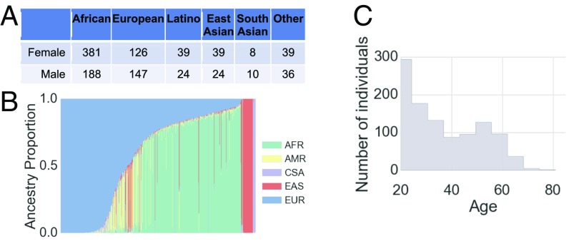
We collected a convenience sample of 1,061 individuals from the San Diego, CA, area. Their genomes were sequenced at an average depth of >30$\times$ (17). The cohort was ethnically diverse, with 569, 273, 63, 63, and 18 individuals who identified themselves as of African, European, Latino, East Asian, and South Asian ethnicity, respectively, and 75 as others (Fig. 1A). The genetic diversity in the San Diego area was reflected in continuous differences in admixture proportions (18) (Fig. 1B). It also included a diverse age range from 18 to 82 y old, with an average of 36 y old (Fig. 1C). Each individual underwent standardized collection of phenotypes, including high-resolution 3D facial images, voice samples, quantitative eye and skin colors, age, height, and weight (Fig. 1). The study was approved by the Western Institutional Review Board, Puyallup, WA. All study participants provided informed consent, allowing research use of their data (see SI Appendix).

Fig. 1.

Study overview. (A) Distribution of self-reported ethnicity in the study. (B) Inferred genomic ancestry proportions for each study participant. Ancestry components are African (AFR), Native American (AMR), Central South Asian (CSA), East Asian (EAS), and European (EUR). (C) Distribution of ages in the study.

Predicting Face and Voice.

Modern facial- and voice-recognition systems reach human-level identification performance (19, 20). Although still in its infancy, genomic prediction of the face may enable identification of a person. We first represented face shape and texture variation using principal components (PC) analysis to define a low-dimensional representation of the face (14, 21–25). Next, we predicted each face PC separately using ridge regression with ancestry information from 1,000 genomic PCs [also equivalent to genomic best linear unbiased prediction from common variation (26)], with sex, BMI, and age as covariates. We undertook a similar procedure using distances between 3D landmarks. A sample of predicted faces is presented in Fig. 2. Predictions for 24 consented individuals are presented in SI Appendix, Fig. S11. We observed that facial predictions reflected the sex and ancestry proportions of the individual.

Fig. 2.

Examples of real (Left) and predicted (Right) faces.

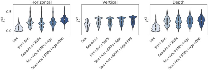
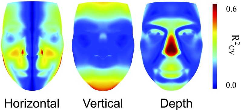
To assess the influence of each covariate on predictive accuracy, we measured the per-pixel $R_{CV}^2$ between observed and predicted faces. Because errors were anisotropic, we separated residuals for horizontal, vertical, and depth dimensions. Fig. 3 shows the distribution of $R_{CV}^2$ along each axis as a function of the model covariates. We observed from this plot that sex and genomic PCs alone explained large fractions of the predictive accuracy of the model. Previously reported single nucleotide polymorphisms (SNPs) related to facial structure (5, 14, 27) did not improve the sex and PC model. In contrast, we found that accounting for age and BMI improved the accuracy of facial structure along the horizontal and vertical dimensions (Fig. 3). To further understand predictive accuracy for the full model, we mapped per-pixel accuracy onto the average facial scaffold (Fig. 4), finding that most of the predictive accuracy was in facial regions that differed the most between African and European individuals (SI Appendix, Fig. S13): Much of the predictive accuracy along the horizontal dimension came from estimating the width of the nose and lips. Along the vertical dimension, we obtained the highest precision in the placement of the cheekbones and the upper and lower regions of the face. For the depth axis, the most predictable features were the protrusions of the brow, nose, and lips. A genome-wide association study (GWAS) on distances between 36 landmarks (SI Appendix, Tables S1 and S2) found no significant associations after correcting for the number of phenotypes tested (SI Appendix and Dataset S1). Because the predictive analysis used the same cohort, we did not use any results from our GWAS to improve (i.e., overfit) predictive models.

Fig. 3.

Violin plots of the per-pixel variation in $R_{CV}^2$ for face shape across three shape axes achieved for different feature sets. Anc refers to 1,000 genomic PCs. SNPs refers to previously reported SNPs related to facial structure (5, 14, 27).

Fig. 4.

Per-pixel $R_{CV}^2$ in face shape for the full model, across three shape axes.

For prediction of voice, we extracted and predicted a 100-dimensional identity-vector and voice pitch embedding (28) from voice samples collected from our cohort. Similar to face prediction, we fitted ridge regression models to each dimension of the embedding. As covariates, we used 1,000 genomic PCs and sex. We were able to predict voice pitch with an $R_{CV}^2$ of 0.70. However, predictions for only 3 of the 100 identity-vector dimensions exceeded an $R_{CV}^2$ of 0.10.

Besides genomic prediction, our method for reidentification used predictions from image and voice embeddings. Face shape, face color, and voice were reasonably predictive of age, sex, and ancestry (Table 1). In summary, we are able to predict variation in face and voice from WGS data and to predict age, sex, and ancestry from face and voice embeddings.

Table 1.

Prediction from images and voice samples

Source trait	Age	Sex	AFR	EUR	EAS	AMR	CSA
Shape	0.82	0.79	0.84	0.78	0.57	0.16	0.11
Color	0.75	0.84	0.89	0.84	0.62	0.24	0.24
Voice	0.62	0.70	0.67	0.38	0.14	0.03	0.02

$R_{CV}^2$ values for age, sex, and five components of genetic ancestry from face shape (shape), face color (color), and voice.

Predicting Age from WGS Data.

Age is a soft biometric that narrows down identity (15). We predicted age from WGS data based on somatic changes that are biologically associated with aging (e.g., telomere shortening). Telomere length can be estimated from WGS data based on the proportion of reads containing telomere repeats (29). We predicted age from estimated telomere length with $R_{CV}^2=\mathrm{\hspace{0.17em}0.29}$ (Fig. 5A). A similar method had been reported to predict age from telomeres with an $R^2$ of 0.05 (29), consistent with our result on 1,960 females from the same cohort that had been sequenced by using the same pipeline as our study cohort (SI Appendix) (30). In addition to telomere length, we were able to detect mosaic loss of the X chromosome with age in women from WGS data. This effect has been reported using in situ hybridization (31). In men, no such effect has been observed, presumably because at least one functioning copy of the X chromosome is required per cell. Additionally, we were able to replicate previous results (32, 33) and detect mosaic loss of the Y chromosome with age in men. Together, telomere shortening and sex chromosome loss, quantified by using sex chromosome copy numbers, were predictive of age, with an $R_{CV}^2$ of 0.44 (mean absolute error ($MAE$) = 8.0 y).

Fig. 5.

(A) Predicted vs. true age. $R_{CV}^2$ for models using features including telomere length (telomeres) and X and Y chromosome copy numbers quantifying mosaic loss (X/Y copy). (B) Predictive performance for height, weight, and BMI using covariate sets composed from predicted age and/or sex, 1,000 genomic PCs, and previously reported SNPs. (C) Predictive performance for eye color. PC projection of observed eye color, the correlation between the first PC of observed values and the first PC of predicted values, and predictive performance of models using different covariate sets composed from three genomic PCs and previously reported SNPs are shown. (D) Predictive performance for skin color. PC projection of observed skin color, the correlation between the first PC of observed values and the first PC of predicted values, and cross-validated variance explained by models using different covariate sets composed from three genomic PCs and previously reported SNPs are shown.

Height, Weight, and BMI Prediction.

To predict height, weight, and BMI, we applied joint shrinkage to previously reported effect sizes (34–36). For height, where we observed the largest predictive power among these traits, a model using reported SNP effects alone yielded $R_{CV}^2=\mathrm{\hspace{0.17em}0.06}$ in males (m) and $R_{CV}^2=\mathrm{\hspace{0.17em}0.08}$ in females (f). Simulations indicated that such predictive performance would result in marginal improvements in discriminative power over random (SI Appendix, Fig. S34). Consequently, models added genomic PCs and sex. As shown in Fig. 5B, we observed a strong performance for the prediction of height ($R_{CV}^2=\mathrm{\hspace{0.17em}0.53}$, $MAE=\mathrm{\hspace{0.17em}4.9}cm$) and weaker performance for the prediction of weight ($R_{CV}^2=\mathrm{\hspace{0.17em}0.14}$, $MAE=\mathrm{\hspace{0.17em}15.6}kg$) and BMI ($R_{CV}^2=\mathrm{\hspace{0.17em}0.17}$, $MAE=\mathrm{\hspace{0.17em}5.3}kg/m^2$).

Eye Color and Skin Color Prediction.

Whereas weight and BMI have complex genetic architecture and have mid to high heritability estimates from 50 to 93% (34, 37), eye color has an estimated heritability of 98% (38), with eight SNPs determining most of the variability (39). Similarly, skin color has an estimated heritability of 81% (40), with 11 genes predominantly contributing to pigmentation (41).

For both eye and skin color, previous models predicted color categories rather than continuous values (10, 13, 42), often by using ad hoc decision rules. To our knowledge, none have used genome-wide variation to predict color. Here, we modeled eye and skin color as 3D continuous RGB values, maintaining the full color variation (see Fig. 5 C and D for eye and skin color, respectively). For both, we calculated per-channel $R_{CV}^2$ of 0.77–0.82.

Linking Genomes to Phenotypic Profiles.

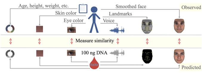
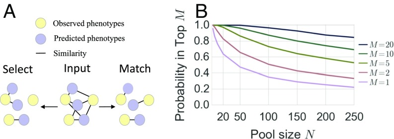
In the previous sections, we presented predictive models for face, voice, age, height, weight, BMI, eye color, and skin color. We integrated each of the predictions as outlined in Fig. 6. In brief, we used predictive models to embed each phenotype and each genome and ranked individuals by their similarity computed from the embeddings listed in SI Appendix, Table S14. Face and voice prediction were modified to use genomic predictions of sex, BMI, and age rather than observed values. We predicted sex, age and ancestry proportions from face and voice as additional variables that could be compared with corresponding genomic predictions ($R_{CV}^2$ in SI Appendix, Tables S3 and S4). Finally, to account for variations in accuracy, we learned an optimal similarity for matching observed and predicted values for each feature set, leading to consistent improvements over naive combination of predictors (SI Appendix, Figs. S26 and S28). To assess the matching performance, we considered the following tasks. Given an individual’s WGS data, we sought to identify that individual out of $N$ suspects whose phenotypes were observed, a problem that we refer to as select at $N$ ($s_N$). In a second scenario, we evaluated whether deidentified WGS samples of $N$ individuals could be matched to their $N$ phenotypic sets (i.e., images and demographic information). This scenario corresponds to the reidentification of genomic databases. We refer to this challenge as match at $N$ ($m_N$). Fig. 7A presents a schematic of $s_N$ and $m_N$. In contrast to $s_N$, where a genome is paired to the most similar phenotypic profile, for $m_N$, each genome was paired to one and only one phenotypic set in a globally optimal manner. That is, we treated $m_N$ as a bipartite graph matching problem and maximized the expected number of correct pairs (6, 43). Table 2 shows $s_N$ and $m_N$ accuracy across feature sets and pool sizes averaged over all possible lineups per CV fold. To further assess the reidentification performance beyond basic demographic information, we include results stratified by gender (SI Appendix, Fig. S29); the largest ethnicity groups, AFR and EUR (SI Appendix, Fig. S30); and gender/ethnicity (SI Appendix, Fig. S31). Corresponding receiver operating characteristic curves are provided in SI Appendix, Figs. S26 and S27. We considered three sets of information: (i) 3D face; (ii) demographic variables such as age, self-reported gender, and ethnicity; and (iii) additional traits like voice, height, weight, and BMI. We found that 3D face alone is most informative, with an $s_{10}$ of 58% (m, 42%; f, 43%; AFR, 32%; EUR, 35%). Ethnicity was second, achieving an $s_{10}$ of 50% (m, 48%; f, 52%). Voice had an $s_{10}$ of 42% (m, 27%; f, 31%; AFR, 29%; EUR, 25%), whereas age, gender, and height/weight/BMI yielded $s_N$ of 20% (m, 19%; f, 20%; AFR, 20%; EUR, 20%), 21% (AFR, 20%; EUR, 20%), and 27% (m, 17%; f, 18%; AFR, 23%; EUR, 24%), respectively. Finally, we integrated these variables to obtain an $s_{10}$ of 74% (m, 65%; f, 65%; AFR, 44%; EUR, 50%). For the full model, $m_{10}$ was 83% (m, 72%; f, 70%; AFR, 47%; EUR, 57%), compared with 64% (m, 44%; f, 46%; AFR, 33%; EUR, 34%) for 3D face alone.

Fig. 6.

Overview of the experimental approach. A DNA sample and a variety of phenotypes are collected for each individual. We used predictive modeling to derive a common embedding for phenotypes and the genomic sample as detailed in SI Appendix, Table S14. The concordance between genomic and phenotypic embeddings are used to match an individual’s phenotypic profile to the DNA sample.

Fig. 7.

Ranking individuals. (A) Schematic representation of the difference between select (best option chosen independently) and match (jointly optimal edge set chosen). Select corresponds to picking an individual out of a group of $N$ individuals based on a genomic sample. Match corresponds to jointly matching a group of individuals to their genomes. (B) Ranking performance. The empirical probability that the true subject is ranked in the top $M$ as a function of the pool size $N$.

Table 2.

Top one accuracy in match and select

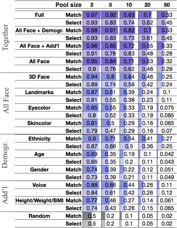Reidentification accuracy in select and match averaged over all possible lineups formed for each CV fold of different pool sizes from 2 to 50 using the various phenotype sets listed in SI Appendix, Table S14.

We evaluated the scenario that tests the probability of including the true individual in a 10-person subset of a random 100-person pool chosen from our cohort. Fig. 7B presents our ability to ensure that an individual is in the top $M$ from a pool of size $N>M$. We ranked the correct individual in the top $M=\mathrm{\hspace{0.17em}10}$ of $N=\mathrm{\hspace{0.17em}100}$ 88% of the time, showing the ability to enrich for persons of interest.

Discussion

We have presented predictive models for facial structure, voice, eye color, skin color, height, weight, and BMI from common genetic variation and have developed a model for estimating age from WGS data. Despite limitations in statistical power due to the small sample size of 1,061 individuals, predictions are sound. Although individually, each predictive model provided limited information about an individual’s identity, we have derived an optimal similarity measure from multiple prediction models that enabled matching between genomes and phenotypic profiles with good accuracy. Over time, predictions will get more precise, and, thus, the results of this work will be of greater consideration in the current discussion on genome privacy protection. Although precision will be gained from larger GWAS contributing common variants, our simulation results indicate that high values of $R^2$ are required to significantly improve identification (SI Appendix, Figs. S33 and S34). These values will likely be obtained by improved phenotyping (e.g., imaging) or from sequencing studies contributing low-frequency variants that have larger effects (44) and discriminate interregional admixture on a finer level (45). Precision will also improve from integration of other experimental sources. For example, age prediction from DNA methylation (46) would be expected to improve performance over a purely genome-based approach.

Today, HIPAA does not consider genome sequences as identifying information that has to be removed under the Safe Harbor Method for deidentification. Based on an assessment of current risks, the latest revision of the Common Rule (01/19/2017; https://www.hhs.gov/ohrp/regulations-and-policy/regulations/finalized-revisions-common-rule) excludes proposed restrictions on the sharing of genomics data. Here, we show that phenotypic prediction from WGS data can enable reidentification without any further information being shared. If conducted for unethical purposes, this approach could compromise the privacy of individuals who contributed their genomes into a database. In stratified analyses, we see that risk of reidentification correlates with variability of the cohort. Although sharing of genomic data is invaluable for research, our results suggest that genomes cannot be considered fully deidentifiable and should be shared by using appropriate levels of security and due diligence.

Our results may also be discussed in the context of genomic forensic sciences. Forensic applications include postmortem identification (47) and the association and identification of DNA from biological evidence (15, 48) for intelligence and law enforcement agencies. In the United States, an average of $\sim$35% of homicides remain unsolved (49). For crimes such as these, DNA evidence (e.g., a spot of blood at a crime scene) may be available (50). In many cases, the perpetrator’s DNA is not included in a database such as the Combined DNA Index System (51). As the field of genomics matures, forensics may adopt approaches similar to this work to complement other types of evidence. Matching DNA evidence to a more commonly available phenotypic set, such as facial images and basic demographic information, would serve to aid cases where conventional DNA testing, database search, and familial testing (52) fails. Today, forensic genomics relies heavily on PCR analyses—in particular, the study of short tandem repeats and characterization of the Y chromosome and mitochondrial DNA haplotypes. The current WGS workflow requires $100ng$ of DNA. However, materials for forensic analyses may be extremely limited, thus confining a broader application of WGS. In these cases, the protocol would need additional cycles of amplification or even whole-genome amplification to achieve sufficient DNA for analysis. In addition, the forensics field is subject to regulations that differ between states and countries.

Materials and Methods

We use the following two-step approach to measure similarity between a deidentified genome $g\in \mathcal{G}$ and a set of identified phenotypic measurements derived from an image and demographic information $p\in \mathcal{P}$ (Fig. 6) (see SI Appendix for details). First, we find a mapping of phenotypes, ${\psi }_{\mathcal{P}}:\mathcal{P}\to {\mathcal{E}}_{\mathcal{P}}$, and a mapping of genomes, ${\varphi }_{\mathcal{P}}:\mathcal{G}\to {\mathcal{E}}_{\mathcal{P}}$, into a common $D$-dimensional embedding-space ${\mathcal{E}}_{\mathcal{P}}\in R^D$. As mappings, we use a combination of PC analysis and predictive modeling. Second, we learn an optimal similarity ${\delta }_{\mathcal{P}}:{\mathcal{E}}_{\mathcal{P}}\times {\mathcal{E}}_{\mathcal{P}}\to ℝ$ that allows comparison of mapped phenotypes ${\psi }_{\mathcal{P}}(p)$ and genomes ${\varphi }_{\mathcal{P}}(g)$.

Learning Embeddings.

For any given phenotype, we have defined suitable embeddings. Phenotypes that are a single number, such as height, weight, or age, are simply represented by their phenotype value. For high-dimensional phenotypes, such as images or voice samples, we have defined embeddings to capture a maximum amount of information relevant for matching. For example, facial images provide information on the shape and the color of the face. Additionally, a facial image may provide information about sex, ancestry, and the age of the person. Consequently, we embedded images into a set of PC dimensions that capture shape and color information, and additional dimensions for sex, ancestry, and age. Having defined an embedding, we learned ${\psi }_{\mathcal{P}}:\mathcal{P}\to {\mathcal{E}}_{\mathcal{P}}$ and ${\varphi }_{\mathcal{P}}:\mathcal{G}\to {\mathcal{E}}_{\mathcal{P}}$ to map phenotypes and genomes into this embedding. In the case of facial images, ${\psi }_{\mathcal{P}}$ is given by face shape and color PC projection of the image and regression models that had been trained to predict sex, age, and ancestry from the image. ${\varphi }_{\mathcal{P}}$ is given by extracting sex and ancestry from the genome, as well as regression models for facial PCs and age. For a list of the embeddings used for different phenotypes, see SI Appendix, Table S14.

Learning a Similarity Function.

Having obtained the embedding functions, we learn an optimal similarity, ${\delta }_{\mathcal{P}}$, that takes embedded phenotype ${\psi }_{\mathcal{P}}(p)$ and genotype ${\varphi }_{\mathcal{P}}(g)$ and outputs a similarity. As a naive similarity ${\delta }_{\mathcal{P}}^{cosine}$, we took the cosine between the vector valued ${\psi }_{\mathcal{P}}(p)$ and ${\varphi }_{\mathcal{P}}(g)$. However, because not all dimensions of ${\mathcal{E}}_{\mathcal{P}}$ can be expected to yield equal amounts of information for judging similarity between phenotypes and genomes, we learned optimally weighted similarity functions ${\delta }_{\mathcal{P}}$ to improve reidentification.

$${\delta }_{\mathcal{P}}\left({\psi }_{\mathcal{P}}\left(p\right),{\varphi }_{\mathcal{P}}\left(g\right)\right)=\sum _{d=1}^D{w}_d\left|{\psi }_{\mathcal{P}}{\left(p\right)}_d-{\varphi }_{\mathcal{P}}{\left(g\right)}_d\right|,$$ [1]

where the weights $w_d$, which reflect the importance of $d$-th dimension of ${\mathcal{E}}_{\mathcal{P}}$, have been trained using a maximum entropy model (53).

References

- 1.Frudakis T. Molecular Photofitting: Predicting Ancestry and Phenotype Using DNA. Elsevier; New York: 2010. [Google Scholar]
- 2.Liu F, et al. A genome-wide association study identifies five loci influencing facial morphology in europeans. PLoS Genet. 2012;8:e1002932. doi: 10.1371/journal.pgen.1002932. [DOI] [PMC free article] [PubMed] [Google Scholar]
- 3.Paternoster L, et al. Genome-wide association study of three-dimensional facial morphology identifies a variant in PAX3 associated with nasion position. Am J Hum Genet. 2012;90:478–485. doi: 10.1016/j.ajhg.2011.12.021. [DOI] [PMC free article] [PubMed] [Google Scholar]
- 4.Adhikari K, et al. A genome-wide association scan implicates DCHS2, RUNX2, GLI3, PAX1 and EDAR in human facial variation. Nature Commun. 2016;7:11616. doi: 10.1038/ncomms11616. [DOI] [PMC free article] [PubMed] [Google Scholar]
- 5.Liu F, et al. Genetics of skin color variation in Europeans: Genome-wide association studies with functional follow-up. Hum Genet. 2015;134:823–835. doi: 10.1007/s00439-015-1559-0. [DOI] [PMC free article] [PubMed] [Google Scholar]
- 6.Humbert M, Huguenin K, Hugonot J, Ayday E, Hubaux JP. De-anonymizing genomic databases using phenotypic traits. Proc Privacy Enhancing Tech. 2015;2015:99–114. [Google Scholar]
- 7.Telenti A, Ayday E, Hubaux JP. On genomics, kin, and privacy. F1000Res. 2014;3:80. doi: 10.12688/f1000research.3817.1. [DOI] [PMC free article] [PubMed] [Google Scholar]
- 8.Erlich Y, Narayanan A. Routes for breaching and protecting genetic privacy. Nat Rev Genet. 2014;15:409–421. doi: 10.1038/nrg3723. [DOI] [PMC free article] [PubMed] [Google Scholar]
- 9.McLaren PJ, et al. Privacy-preserving genomic testing in the clinic: A model using HIV treatment. Genet Med. 2016;18:814–822. doi: 10.1038/gim.2015.167. [DOI] [PMC free article] [PubMed] [Google Scholar]
- 10.Hart KL, et al. Improved eye-and skin-color prediction based on 8 SNPs. Croat Med J. 2013;54:248–256. doi: 10.3325/cmj.2013.54.248. [DOI] [PMC free article] [PubMed] [Google Scholar]
- 11.Craig DW, et al. Assessing and managing risk when sharing aggregate genetic variant data. Nat Rev Genet. 2011;12:730–736. doi: 10.1038/nrg3067. [DOI] [PMC free article] [PubMed] [Google Scholar]
- 12.Liu F, Wen B, Kayser M. Colorful DNA polymorphisms in humans. Semin Cell Dev Biol. 2013;24:562–575. doi: 10.1016/j.semcdb.2013.03.013. [DOI] [PubMed] [Google Scholar]
- 13.Spichenok O, et al. Prediction of eye and skin color in diverse populations using seven SNPs. Forensic Sci Int Genet. 2011;5:472–478. doi: 10.1016/j.fsigen.2010.10.005. [DOI] [PubMed] [Google Scholar]
- 14.Claes P, et al. Modeling 3D facial shape from DNA. PLoS Genet. 2014;10:e1004224. doi: 10.1371/journal.pgen.1004224. [DOI] [PMC free article] [PubMed] [Google Scholar]
- 15.Kayser M. Forensic DNA phenotyping: Predicting human appearance from crime scene material for investigative purposes. Forensic Sci Int Genet. 2015;18:33–48. doi: 10.1016/j.fsigen.2015.02.003. [DOI] [PubMed] [Google Scholar]
- 16.Gymrek M, McGuire AL, Golan D, Halperin E, Erlich Y. Identifying personal genomes by surname inference. Science. 2013;339:321–324. doi: 10.1126/science.1229566. [DOI] [PubMed] [Google Scholar]
- 17.Telenti A, et al. Deep sequencing of 10,000 human genomes. Proc Natl Acad Sci USA. 2016;113:11901–11906. doi: 10.1073/pnas.1613365113. [DOI] [PMC free article] [PubMed] [Google Scholar]
- 18.Alexander DH, Novembre J, Lange K. Fast model-based estimation of ancestry in unrelated individuals. Genome Res. 2009;19:1655–1664. doi: 10.1101/gr.094052.109. [DOI] [PMC free article] [PubMed] [Google Scholar]
- 19.Taigman Y, Yang M, Ranzato M, Wolf L. Proceedings of the IEEE Conference on Computer Vision and Pattern Recognition. IEEE; New York: 2014. Deepface: Closing the gap to human-level performance in face verification; pp. 1701–1708. [Google Scholar]
- 20.Dehak N, Kenny PJ, Dehak R, Dumouchel P, Ouellet P. Front-end factor analysis for speaker verification. IEEE Trans Audio Speech Lang Process. 2011;19:788–798. [Google Scholar]
- 21.Turk M, Pentland A. Eigenfaces for recognition. J Cogn Neurosci. 1991;3:71–86. doi: 10.1162/jocn.1991.3.1.71. [DOI] [PubMed] [Google Scholar]
- 22.Turk G, O’brien JF. Modelling with implicit surfaces that interpolate. ACM Trans Graph. 2002;21:855–873. [Google Scholar]
- 23.Belongie S, Malik J, Puzicha J. Shape matching and object recognition using shape contexts. IEEE Trans pattern Anal Mach Intell. 2002;24:509–522. doi: 10.1109/TPAMI.2005.220. [DOI] [PubMed] [Google Scholar]
- 24.Amberg B, Romdhani S, Vetter T. Optimal step nonrigid ICP algorithms for surface registration in 2007. IEEE Conf Computer Vis Pattern Recognit. 2007:1–8. [Google Scholar]
- 25.Guo J, Mei X, Tang K. Automatic landmark annotation and dense correspondence registration for 3D human facial images. BMC Bioinformatics. 2013;14:232. doi: 10.1186/1471-2105-14-232. [DOI] [PMC free article] [PubMed] [Google Scholar]
- 26.Meuwissen THE, Hayes BJ, Goddard ME. Prediction of total genetic value using genome-wide dense marker maps. Genetics. 2001;157:1819–1829. doi: 10.1093/genetics/157.4.1819. [DOI] [PMC free article] [PubMed] [Google Scholar]
- 27.Qiao L, et al. 2016. Detecting genome-wide variants of Eurasian facial shape differentiation: DNA based face prediction tested in forensic scenario. bioRxiv: 10.1101/0062950.
- 28.Hasan R, Jamil M, Rabbanil G, Rahman S. Proceedings of the 3rd International Conference on Electrical & Computer Engineering. IEEE; New York: 2004. Speaker identification using mel frequency cepstral coefficients; pp. 565–568. [Google Scholar]
- 29.Ding Z, et al. Estimating telomere length from whole genome sequence data. Nucleic Acids Res. 2014;42:e75. doi: 10.1093/nar/gku181. [DOI] [PMC free article] [PubMed] [Google Scholar]
- 30.Long T, et al. Whole-genome sequencing identifies common-to-rare variants associated with human blood metabolites. Nat Genet. 2017;49:568–578. doi: 10.1038/ng.3809. [DOI] [PubMed] [Google Scholar]
- 31.Hisama F, Weissman SM, Martin GM. Chromosomal Instability and Aging: Basic Science and Clinical Implications. CRC; Boca Raton, FL: 2003. [Google Scholar]
- 32.Jacobs KB, et al. Detectable clonal mosaicism and its relationship to aging and cancer. Nat Genet. 2012;44:651–658. doi: 10.1038/ng.2270. [DOI] [PMC free article] [PubMed] [Google Scholar]
- 33.Forsberg LA, et al. Mosaic loss of chromosome Y in peripheral blood is associated with shorter survival and higher risk of cancer. Nat Genet. 2014;46:624–628. doi: 10.1038/ng.2966. [DOI] [PMC free article] [PubMed] [Google Scholar]
- 34.Dubois L, et al. Genetic and environmental contributions to weight, height, and BMI from birth to 19 years of age: An international study of over 12,000 twin pairs. PLOS one. 2012;7:e30153. doi: 10.1371/journal.pone.0030153. [DOI] [PMC free article] [PubMed] [Google Scholar]
- 35.Locke AE, et al. Genetic studies of body mass index yield new insights for obesity biology. Nature. 2015;518:197–206. doi: 10.1038/nature14177. [DOI] [PMC free article] [PubMed] [Google Scholar]
- 36.Wood AR, et al. Defining the role of common variation in the genomic and biological architecture of adult human height. Nat Genet. 2014;46:1173–1186. doi: 10.1038/ng.3097. [DOI] [PMC free article] [PubMed] [Google Scholar]
- 37.Silventoinen K, et al. Heritability of adult body height: A comparative study of twin cohorts in eight countries. Twin Res. 2003;6:399–408. doi: 10.1375/136905203770326402. [DOI] [PubMed] [Google Scholar]
- 38.Bito LZ, Matheny A, Cruickshanks KJ, Nondahl DM, Carino OB. Eye color changes past early childhood: The Louisville twin study. Arch Ophthalmol. 1997;115:659–663. doi: 10.1001/archopht.1997.01100150661017. [DOI] [PubMed] [Google Scholar]
- 39.Mushailov V, Rodriguez SA, Budimlija ZM, Prinz M, Wurmbach E. Assay development and validation of an 8-SNP multiplex test to predict eye and skin coloration. J Forensic Sci. 2015;60:990–1000. doi: 10.1111/1556-4029.12758. [DOI] [PubMed] [Google Scholar]
- 40.Clark P, Stark A, Walsh R, Jardine R, Martin N. A twin study of skin reflectance. Ann Hum Biol. 1981;8:529–541. doi: 10.1080/03014468100005371. [DOI] [PubMed] [Google Scholar]
- 41.Sturm RA. Molecular genetics of human pigmentation diversity. Hum Mol Genet. 2009;18:R9–R17. doi: 10.1093/hmg/ddp003. [DOI] [PubMed] [Google Scholar]
- 42.Maroñas O, et al. Development of a forensic skin colour predictive test. Forensic Sci Int Genet. 2014;13:34–44. doi: 10.1016/j.fsigen.2014.06.017. [DOI] [PubMed] [Google Scholar]
- 43.Galil Z. Efficient algorithms for finding maximum matching in graphs. ACM Comput Surv. 1986;18:23–38. [Google Scholar]
- 44.Zuk O, et al. Searching for missing heritability: Designing rare variant association studies. Proc Natl Acad Sci USA. 2014;111:E455–E464. doi: 10.1073/pnas.1322563111. [DOI] [PMC free article] [PubMed] [Google Scholar]
- 45.Leslie S, et al. The fine-scale genetic structure of the british population. Nature. 2015;519:309–314. doi: 10.1038/nature14230. [DOI] [PMC free article] [PubMed] [Google Scholar]
- 46.Horvath S. DNA methylation age of human tissues and cell types. Genome Biol. 2013;14:R115. doi: 10.1186/gb-2013-14-10-r115. [DOI] [PMC free article] [PubMed] [Google Scholar]
- 47.INTERPOL . Disaster Victim Identification Guide. INTERPOL; Lyon, France: 2014. [Google Scholar]
- 48.Sulem P, et al. Genetic determinants of hair, eye and skin pigmentation in europeans. Nat Genet. 2007;39:1443–1452. doi: 10.1038/ng.2007.13. [DOI] [PubMed] [Google Scholar]
- 49.Smith EL, Cooper A. Homicide in the US Known to Law Enforcement, 2011. Department of Justice Bureau of Justice Statistics; Washington, DC: 2013. [Google Scholar]
- 50.Peterson J, Sommers I, Baskin D, Johnson D. The Role and Impact of Forensic Evidence in the Criminal Justice Process. National Institute of Justice; Washington, DC: 2010. pp. 1–151. [Google Scholar]
- 51. Federal Bureau of Investigation (2016) Frequently asked questions (FAQs) on the CODIS program and the national DNA index system. Accessed August 8, 2017.
- 52.Bieber FR, Brenner CH, Lazer D. Human genetics. Finding criminals through DNA of their relatives. Science. 2006;312:1315–1316. doi: 10.1126/science.1122655. [DOI] [PubMed] [Google Scholar]
- 53.Och FJ, Ney H. Proceedings of the 40th Annual Meeting on Association for Computational Linguistics. Association for Computational Linguistics; Stroudsburg, PA: 2002. Discriminative Training and Maximum Entropy Models for Statistical Machine Translation; pp. 295–302. [Google Scholar]
Associated Data
This section collects any data citations, data availability statements, or supplementary materials included in this article.